Calibration of a multivariate PARMA model for the ottawa river system.

Author Role:

Title, Monographic: Calibration of a multivariate PARMA model for the Ottawa river system Translated Title:

Reprint Status: Edition:

Author, Subsidiary: Author Role:

Place of Publication: Québec Publisher Name: INRS-Eau Date of Publication: 1995

Original Publication Date: Février 1995 Volume Identification:

Extent of Work: iii, 85

Packaging Method: pages incluant 3 annexes Series Editor:

Series Editor Role:

Series Title: INRS-Eau, Rapport de recherche Series Volume ID: 432

Location/URL:

ISBN: 2-89146-428-1

Notes: Rapport annuel 1994-1995

Abstract: Rapport rédigé pour Hydro-Québec

Call Number: R000432

CALmRATION OF A MULTIVARIATE PARMA MODEL FOR THE OTTAWA RIVER SYSTEM

Report prepared for HYDRO-QUEBEC by Peter F. Rasmussen Louis Mathier Jose Salas Laura Fagherazzi Jean-Claude Rassam

Institut national de la recherche scientifique, INRS-Eau

2800, rue Einstein, Case postale 7500, SAINTE-FOY (Québec) G1V 4C7

Rapport de recherche R-432

CALIBRATION OF

A MULTIVARIATE PARMA MODEL FOR THE OTTAWA RIVER SYSTEM

1 Introduction ... . 1

2 Model selection criteria ... .. , ... 5

3 Estimation methods ... 9

3.1 Introduction ... 9

3.2 Estimation

by

the method ofleast squares ... 9

3.3 Estimation

by

the method ofmoments ... 9

3.4 Estimation using the MATLAB/ ARMAX function ... ... 11

3.5 Comparison of estimation method ... 12

4 Descri{ttion of CSU5 ... 15

5 Results of single-site estimation ... ... 17

5.1 Introduction ... 17

5.2 North East region ... 19

5.3 North West region ... 19

5.4 East region ... 20

5.5 Central region ... 20

5.6 South region ... 20

5.7 Summary of results ... ... 20

6 Estimation of the cross-covariance ofresiduals ... 25

6.1 Introduction ... 25

6.2 Moment estimation of spatial correlations ... ... 27

7 Results of multi-site estimation ... 31

8 Concluding remarks ... 3 7 9 References ... ... 39

Appendix A. Periodic multivariate Yule-Walker equations ... 43

Appendix B. MATLAB programs ... 45

List of figures

Figure 3.1 Periodic covariance function of a moment estimated P ARMA model

for the Central region ... 10 Figure 3.2 Periodic standard deviation of simulated flows for the South region ... 13 Figure 3.3 Lag 1 week-to-week correlation ofsimulated flows for the South region. 14 Figure 5.1 Observed lag 1 to 4 week-to-week correlation in the Central region ... 17 Figure 7.1 Observed and fitted cross-correlation offlows ... 35 Appendix C Periodic variance and periodic autocorrelation offitted models ... 57

Table 5.1 Lenght of data series ... 18 Table 5.2 Estimated P ARMA(p,q)-parameters for the five regions

in the Ottawa River ... 21 Table 7.1 Elements of the periodic covariance matrices ofresiduals ... 32

1

INTRODUCTION

The present report summarizes various aspects of the development and calibration of a multivariate P ARMA model for the Ottawa River system, or, more precisely, for five regions in that system. The overall objective of the study is to develop a generator of daily simultaneous flows at 30 sites. The generation of a large number of multi-site flow sequences for input to current management models permits to study the reliability of the system, both in terms of hydropower production and in terms of adequacy of the hydraulic installations. The main interest in the current project is the reliability assessment of existing constructions such as dams, spillways, dikes, etc., vis-à-vis extreme floods. Floods occur over a relatively short period of time, in Quebec usually in the spring as a result of snow melt. This is why it is necessary to consider time-steps as small as one day. Since the P ARMA type model is unsuitable for generating daily flows and also is practically limited by the number of sites that can be handled, it has to be combined with various disaggregation models. In the present report, only one component of the flow generator is considered, namely a 5-region, weekly P ARMA model. Generated weeklY regional flows will be disaggregated spatially to each site in the region and to a daily time step, but that part of the generator is not described here. The delineation of 27 gauged sites in the Ottawa River system into five regions has been carefully done with the emphasis on maximizing the statistically similarity of sites within regions. This work is described in Mathier et al. (1995). Although no particular attention was paid to the geographical location of the sites, the five regions turned out to be geographically contiguous. They will in the following be referred to as North West (NW), North East (NE), East (E), Central (C), and South (S) regions.

The distributions of aggregated weekly flows in the five regions have been carefully examined and transformed to normality (I. Grygier, personal communication). The results presented in the following deal only with the transformed data space. Although a good model performance in the transformed data space does not guarantee an equally good performance in real space, it is generally acknowledged that for a model to perform well in real space, it must do weil in the transformed space. Rence, the objective ofthis part of the project will be to identifY the MoSt adequate model for the transformed data.

The models considered here are the class of multivariate P ARMA(p,q) models (lleriodic ,ilutoregressive moving ,ilverage). The data are assumed normalized and standardized to zero Mean and unit variance, but even after removal of the periodic Mean and variance, the data

senes may still exhibit periodicity in the week-to-week correlations. Therefore it is necessary to consider a model with time-varying parameters, such as the multivariate P ARMA models, whose general form is:

p q

XV;t =

L

<Di.'tXV;t-i + sv.'t -

L

9 j.'tsv.'t-j (1)

~1 ~1

The model relates the present flows at n sites (elements of vector x) to the p previous flows and to the q previous innovations. The model and its special cases will be described in detail later. In its general form, the parameter matrices <D~'t and

9

1.'t are allowed to be full. A substantial simplification can be obtained by assuming that these matrices are diagonal (Salas et al., 1980). This uncouples the equations and permits to model each (aggregated) site independently. The spatial dependence is introduced by generating innovation vectors with correlated elements. This type of model, commooly denoted contemporaneous, permits in principle to preserve explicitly the spatial correlation of flows at lag 0, whereas there is no explicit provision for preserving correlations at higher lags. Rowever, contemporaneous models have been used in several studies and are generally found to yield good results.

The periodicity of the parameters and statistics related to them introduces sorne difficulties in identifying the appropriate model order. Classical identification techniques for stationary Box-Jenkins ARMA models are not directIy applicable to seasonal models. The autocorrelation function and the partial autocorrelation function, which are the usual tools for identifying the orders of stationary models, are meaningless when seasonality in the model parameters is present. One can gain some insight by looking at the correlations between periods, but in the case of weekly flows, an exhaustive analysis would be very tedious. Moreover, one cannot expect to arrive at a unique conclusion as to which values of p and q should be used, since generally the correlation pattern depend on the period. The approach taken here is the trial-and-error method. Some a priori chosen models are fitted to the observed data and their performances are evaluated and compared. With the limited data available for the Ottawa River, it is suggested that models beyond P ARMA(2,2) should not be considered. The P ARMA(2,2) model defines a class consisting of P ARMA(p,q) models with max{p,q} ~2. This class comprises among others the popular PARMA(I,O) and PARMA(l,l) models, as weIl as the PARMA(2,1) model. The PARMA(I,I) model is generally found to perform better than the PARMA(2,0) model which is the reason why the latter is not used in this study. PARMA(2,1) models are generally preferable to PARMA(I,2) model, and ooly the former is considered here. Rence, four PARMA models constitute the group of candidates to be examined in this study.

1 Introduction 3

The first part of this report describes properties of the univariate model. Chapter 2 presents the criteria on which we based the model selection. Chapter 3 describes the three different estimation methods that were considered in this study and a comparison between them. Chapter 4 contains a brief description of the program CSU5 which eventually was used to calibrate the P ARMA models. In Chapter 5, we present the results of the calibration of the univariate models.

In the second part of the report, the spatial dimension of the multivariate model is considered. The method of moments was used to estimate the cross-covariance matrices of residuals. This new method for calibrating higher-order contemporaneous models is described in detail in Chapter 6. In Chapter 7, we present the results of the spatial estimation. A few concluding remarks are given in Chapter 8.

2

MODEL SELECTION CRITERIA

In the following, we consider the case of univariate P ARMA models and the problem of determining the appropriate model order. As mentioned in the introduction, Most of the classical methods for model identification do not apply to periodic models, so one usually has to base the choice of model order on a trial-and-error search. The parameters of each considered model is estimated, and one May compute various statistical properties of interest and perform a global comparison of the involved models using the historical data series as reference. Sorne of the properties that one would usually examine are the periodic means, variances, and period-to-period correlations (periodic autocorrelation). In the transformed data space, the periodic means can usually be reproduced exactly (identical to the historical)l, whereas the periodic variances and auto correlation may be more or less close to the historical values used to calibrate the model. Commonly, model properties are obtained by generating long series of flow data. Especially if data have been re-transformed to real space, this is the most straightforward method for deriving the statistical properties of the model. However, for model development, in particular the selection of model order, it May suffice to examine the statistical properties in the transformed data space. Generally, one cannot expect a model to perform well in real space, if it fails to perform weil in the transformed space (Stedinger, 1981). In this study, an analytical technique, based on the periodic Yule-Walker equations, are used to compute the periodic variance and autocorrelation in the transformed data space. This technique is described below.

The univariate P ARMA(2,2) model relates the present flow to preceding flows and innovations by the following functional relationship

2 2

Xy,'t =

L

cl>i,'tXy,'t-i

+

8 y,'t -

Le

j,'t8 y,'t_j (2)

i=1 j=1

where Xy,'t represents the normalized and standardized flow in year v, period t, cl>i,'t are

autoregressive parameters depending on the specific period of the year, and

e

i 't are moving

. average parameters, also depending on the period. It is assumed that there are 0) periods in

the year. Due to the normalization of the flows, the innovations, 8y't' are normally

distributed. Moreover, since the data are assumed standardized to zero Mean and unit variance, the innovations also have zero Mean. The variance of the innovations is denoted

1 Here the term "reproduced exactly" does not imply that each generated series has the same mean as the

historical series, but rather that the expected value of the rnean is identical to the historical rnean. Sarne comment applies to the variance and correlations.

g't and generally depends on the period. Due to the limited amount of data available for calibration, it may be appropriate to consider also models of lower order. Popular sub-models are the PARMA(1,O) and PARMA(l,l), which in many cases provide a satisfactory description of the correlation structure of observed flows. However, when the considered time scale is very short (as for example in the case of weekly flows), the seasonal autocorrelation structure may exhibit irregularities which cannot be adequately captured by low-order P ARMA models. This is why we adopt the P ARMA(2,2) as a general c1ass of models that comprises itself and any submodel, i.e. any PARMA(p,q) model with

max{p,q} S

2.

The values of the parameters of a PARMA(p,q) model uniquely define the covariance structure of the model through the so-called periodic Yule-Walker equations which for the P ARMA(2,2) model read (Appendix A):

m't (0) = <l>1.'tm't (1) + <l>2.'tm't (2) + g't - 9_{1.'tg·t-! [<I>I.'t -} 9_1.'t]

- 9

2.'tg't-2 [<I>I.'t<l>I.'t-1 - <l>1.'t

9

1.'t-1 + <l>2.'t -

9

2.'t] m't(l)

=

<l>1.'tm't-1 (0) + <l>2.'tm't-1 (1) -

9

1.'tg't-1 -

9

2.'tgt-2 [<I>I.'t-1 -

9

1.'t-1] mt(2)

=

<l>1.tmt-l(l) + <l>2.tmt-2(0) - 92.tgt-2 k>2 (3 a) (3b) (3c) (3d)

where the periodic autocovariance function is defined as m'tO)

=

E[X't X't-J The above equations are valid for any submodel of the P ARMA(2,2) by setting particular parameters equal to zero. For instance, the periodic Yule-Walker equations corresponding to a PARMA(2,1) are obtained by setting 9_{2.'t equal to zero. The periodic Yule-Walker} equations serve an important purpose by allowing a fast and straightforward calculation of the periodic variance and the periodic auto correlation corresponding to a given estimated model. Equation (3c) can be used to remove m't(2) from (3a). After sorne manipulations, the first two periodic Yule-Walker equations can be written

A

2 A A A

-<I>2.'tm't-2 (0) + m't (0) - <l>1.t<l>2.'tm't-1 (1) - <l>1.'tm't (1)

= g't

-êl.'tg't-I[~I.'t

-êl.'t

]-ê2.'tg't-2[~I.'t~I.'t-1 -~I.'têl.'t-I +2~2.'t

-ê

2.'t]

(4a)

-~I.'tm't_1

(0) -

~2.'tm't-1

(1)

+

mt (1) = -êl.'tg't-I -

ê

2.'tg't-2

[~I.'t-I

- ê l.t_1 ] (4b) where "J\lI is used to designate particular estimates. It is seen that the above equations constitute a linear system of2c.o equations with 2c.o unknowns, namely m't(O) and m't(1) for

2 Model selection criteria 7

autocorrelation function can then be constructed from (3c-d). It is useful to emphasize that the implementation of (4a-b) aIso permits to evaluate the properties of any submodel of P ARMA(2,2) by equating particular parameters to zero.

The above procedure provides an effective means to compare different model options and to guide in the selection of the most adequate. For example, one may wish to compare a PARMA(1,l), a PARMA(2,1), and a PARMA(2,2) for modeling weekly data at a given location. The first step is to obtain parameter estimates for each model considered, for example by one of the methods described in the next section. Then the periodic variances and autocovariances are computed from (4a-b) and plotted along with the corresponding historical values and a graphical comparison can be made.

The above procedure constitutes the main basis for our model selection. There are other properties that could be examined as weIl, including stationarity conditions and whiteness of the residual series.

3

ESTIMATION METROnS

3.1 Introduction

Prior to undertaking the task of estimating and identifying the appropriate models for the five regions in the Ottawa River, a preliminary analysis of different estimation techniques was made. This analysis led to the conclusion that the method of least squares, as implemented in the software CSU5 developed by the research group of J. Salas at Colorado State University, provided results that were acceptable to aIl participants in the project, and the CSU5 was consequently selected and used for model calibration. However, for completeness, the three estimation alternatives we examined are briefly described here.

3.2 Estimation

by

the method of least squares

The LS estimators are the set of parameters that minimizes the sum of squared residuals, i.e. (assuming a P ARMA(p,q)-model)

N fil

[ p

q

]2

{~i,'t,ej,'t} for which ~ ~ Xv,t - ~~i,tXv,t-i

+

~ej,t8v,t_j is minimum

v=1 t=1 1=1 )=1

The estimate of the residual variance, gt' is obtained directly from the series of residuals. U sually one omits the first p data from the summation, because the p preceding values are unknown (Box and Jenkins' back forecast method do es not apply to periodic series). The fust q innovations are commonly set to zero. The LS method is fairly straightforward, but very computer intensive. The LS method as implemented in CSU5 is described in more detail in the next section.

3.3 Estimation

by

the method of moments

The moment estimators of the parameters of a P ARMA(p,q) model are the solution to the fust p+q

+

1 periodic Yule-Walker equations in which the periodic auto covariance function is computed from the data. Hence, if a moment solution exists, the corresponding model preserves exactly the variance plus the lagged correlations up to order p + q. For low-order PARMA-models, a moment solution is fairly straightforward (Salas et aL, 1982), but if the order of the moving average component of the model exceeds one, then an analytical solution is not available, and even with numerical means, it seems impossible to obtain a solution (Bartolini and Salas, 1993). Therefore, in our study moment solutions were restricted to PARMA(1,O), PARMA(l,l), and PARMA(2,1) models. Unfortunately, in the

Lag 1 correlation 1.0 0.8 0.6 0.4 0.2 0.0 0 4 8 12 16 20 24 28 32 36 40 44 48 52 Lag 2 correlation 1.0 0.8 0.6 0.4 0.2 0.0 -0.2 -0.4 -0.6 0 4 8 12 16 20 24 28 32 36 40 44 48 52 Lag 3 correlation 1 . 0 , . . . - - - , 0.8 0.6 0.4 0.2 ----... . ... . 0.0 + - . - - - 1 1 - - - 1 - - - 1 -0.2 . __ ... -_ ... . -0.4 -._ ... -... _... . ... . -0.6 .-.. --.... --.-... ----... -... _ ... . -O.8+rHH~++rrHH~+rH4~~HH4+++HH~++rH~++HH~~

o

4 8 12 16 20 24 28 32 36 40 44 48 52 Lag 10 correlation 0.8 0.6 0.4 0.2 0.0 -0.2 -0.4 1 4 . 7 10 13 16 19 22 25 28 31 34 37 40 43 46 49 52

Figure 3.1 Periodic covariance function of a moment estimated

3 Estimation methods 11

case of P ARMA(I, 1) and P ARMA(2, 1) models a moment solution may not exist. When calibrating the models, some of the residual variances may tum out negative, indicating that there is no feasible solution to the periodic Yule-Walker equations. When applying the method of moments to the Ottawa River data, it was found necessary to smooth the periodic autocorrelation in order to obtain feasible solutions. A Fourier analysis showed that two harmonics were generally enough to de scribe adequately the periodic autocorrelations, except for the spring flood period. Hence, in our approach we first replaced the data during the flood period with typical values prior to and after the flood period. The coefficients of the tirst two harmonics were determined. Then the irregular correlations in the flood season were inserted in the smoothed periodic autocorrelation function, and the resulting function was used to calibrate the P ARMA-model.

The above approach was applied to the data from the five regions in the Ottawa River. Results from fitting a PARMA(I,I) to the Central region is shown in Figure 3.1. The variance, and the lags 1 and 2 of the transformed data are reproduced exactly (Le. identical to the historical, transformed series.) It is particularly interesting to study the performance of higher order lags which are not explicitly preserved. It is seen that up to at least lag 10, the P ARMA(I, 1 )-model provides an excellent description of the correlation structure.

One obvious advantage of smoothing the periodic auto correlation functions is that the number of independent parameters can be substantially reduced. For example, a PARMA(I,I)-model contains 3co-parameters, which, in the case ofweekly data, means 156 parameters. Since the fitting of parameters to smoothed periodic autocorrelations functions results in smoothed parameters, one can reduce the number of "independent" parameters to two times the number of harmonics considered plus the number of original correlations used during the flood period (in addition to the means, variances, and transformation parameters ).

3.4 Estimation using the MATLAB/ARMAX function

A third method for estimating the parameters of PARMA(2, 2) models was suggested and developed by Mrs. L. Fagherazzi, Hydro-Quebec. It is based on the ARMAX subroutine in MATLAB's System Identification Toolbox. The key idea of this approach is to estimate the parameters of each season independently of the other seasons, ignoring the functional relationship between the moving average parameters of adjacent periods, but allowing for a

fast and simple estimation. The first step is to sequentially extract one column from the data matrix given by:

XIJ _{X I2 X 13} x_lm

X 21 X 22 X 23 X 2m

The two preceding columns are used as exogenous input series (sorne adjustment is needed for the tirst two periods), and the series of flows in a particular period, with length equal to the number of years available for the study, is modeled by a moving average process of order 2. The estimation is based on the method of least squares.

It was found that the estimates of the autoregressive parameters is equivalent to those one would obtain by fitting a traditional P AR(2) model with either the method of moments or the method ofleast squares (autoregressive parameters generally do not pose any estimation problems). The meaning of the moving average parameters is somewhat obscure, since they do not relate directly to the original time series, but rather to the series of one period's flow over n years in which there is no significant autocorrelation

3.5 Comparison of estimation methods

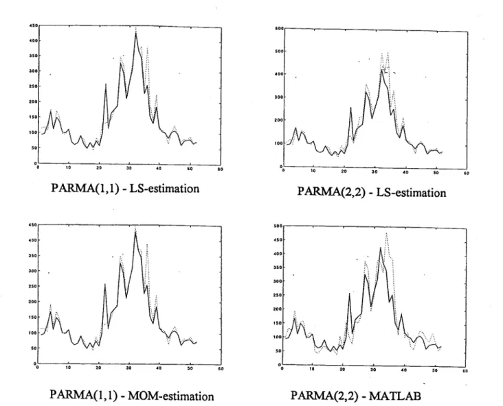
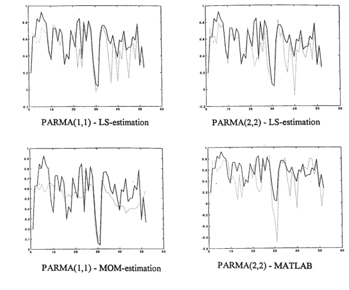
In order to choose the most satisfactory estimation method, a simulation study was carried out, in which the three methods described above were used to calibrate the data series for the South region. The performance of each method was evaluated by generating, for each of the three estimation methods and for various model orders, 1000 series of 23 years of weekly data (corresponding to the length of the historical series) and by computing various statistics in the real data space. These statistics comprised periodic means, variances, lag 1 week-to-week correlations, annual mean, annual maximum, and the distribution of the annual maximum. It was found that in certain periods, the re-transformation had a significant impact on the preservation of statistics. It is well-known that a good preservation of correlations in the transformed data space does not guarantee a good preservation of correlations in real space. However, in principle it should be possible to preserve the periodic real means exactly, but sorne departure was observed in the beginning of the year. This can only be ascribed to the transformation. Also the standard deviation was in sorne cases way off (Figure 3.2). Figure 3.3 shows the average lag 1 week-to-week correlation for a PARMA(I,I)/LS, a PARMA(I,I)/MOM, and a PARMA(2,2)/MATLAB model. Not

3 Estimation methods 500 '00 300 200 °0~--~tO--~20~~3~0--~'O--~S~0--~.0 _{~~--~tO--~20~~3~0--~40~~S~0--~'0}

PARMA(l,l) - LS-estimation _{P ARMA(2,2) - LS-estimation}

~~--~tO--~20~~3~0--~'O----S~0--~'0 _{~~--~tO---7.20~~3~0--~'0----5~0--~'0}

PARMA(I,I) - MOM-estimation PARMA(2,2) -MATLAB

Figure 3.2 Periodic standard deviation of simulated flows for the South region. (dotted lines represent simulated values)

13

surprisingly, it is seen that the MATLAB-method results in a po or preservation of the correlation structure. Because of the smoothing of correlations in the case of estimation.by the method of moments, the generated mean correlations are also fairly smooth as opposed to the model based on LS-estimation, in which the periodic real correlations fluctuate, sometimes very close to, but other times quite away from the historical value. The choice between the LS-method and the MOM-method is not evident. After a careful study of the different statistical characteristics of series generated with the three methods, it was decided to adopt the LS-method for estimating the parameters of the five regional series in the Ottawa River.

10 20 30 .0 50 '0 .O.20L----:,~0 --~2~0 --~30~--~.0;----~SO;---:.'O

PARMA(1,1) - LS-estimation P ARMA(2,2) - LS-estimation

0,' o .• o .• ·0.2 -0.4 .0.6 ooL----,~0--~2~0--~.~0--~.0~--~SO~~.0 .O.80L----:,~0· --~20~--~30;----~.0;----7.S0;---:..0

PARMA(1,1) - MOM-estimation P ARMA(2,2) - MATLAB

Figure 3.3 Lag 1 week-to-week correlation ofsimulated flows for the South region (dotted lines represent simulated values)

4

DESCRIPTION OF

CSU5

CSU5 is a computer software developed at Colorado State University by

J.

Salas and others for calibration of P ARMA models. The program permits to estimate the parameters of several types of periodic models, including the P ARMA(p,q). The program was originally written for application to monthly flows, so the code had to be revised for the current project, in which weekly data are used.

Parameters are estimated by the LS method, briefly described in the preceding chapter. A method of moment solution is used as starting point in the search for a minimum. Initially, the program attempts to estimate a PARMA(l,l)-model by the method of moments. If a solution does not exist, a P ARMA(l,O) moment solution is used as starting values. With an initial estimation of the parameters, the Powell method of direct search is invoked to find the set of parameters that minimizes the sum of squared residuals. The p flows and q innovations preceding the first data (year 1, period 1) is set to zero, and the objective function to be minimized is therefore a sum of nro terms, where n is the number of years. The search terminates when a user-specified accuracy has been attained. The variance of the residual series is used as estimator of gT .

The program provides a variety of outputs such as periodic means and variances of the input series and of the residual series, periodic auto correlation structure, and statistics of the aggregated annual flows. The pro gram aIso tests for whiteness of residuals and for stationarity of the solution. The program, however, does not provide output of the periodic autocovariance function corresponding to the solution. Using MATLAB, we implemented a routine for calculating this important property following the procedure described in Chapter 2.

When estimating the parameters of P ARMA(2,2)-models, the program tumed out to be quite sensitive to the particular computer on which it was run, and also to the Fortran compiler used to compile the source code. A series of test runs based on the same monthly data set were made on ditferent computers and with ditferent compilers in order to examine the ditferences in the solutions. Although the estimated parameters ditfered substantially, the periodic autocovariance structures of the estimated models were quite similar, and it was consequently found impossible to conclu de that any particular computer/compiler combination was significantly superior to the others. Since no particular preference could be

attributed to a specific computer, it was decided to use a PC, on which the manipulation of data is more tractable than on a mainframe. The instability in the solution can be explained by the high dimensions of the PARMA(2,2)-model. In fact, the objective function supposedly is very flat around the minimum, indicating that a large number of solutions may yield virtually identical results in terms of periodic autocovariance structure. The use of high-order models represents one particular point of view in modeling, namely that the large number of parameters and the corresponding instability in the solution is unimportant as long as the covariance structure of the model reasonably well describes the observed historical correlations.

5

RESULTS OF SINGLE-SITE ESTIMATION

5.1 Introduction

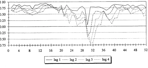
As mentioned in the introduction, our approach to estimating the parameters of the univariate P ARMA-models is the trial-and-error method. Four models, namely the PARMA(l,O), PARMA(l,l), PARMA(2,1), and PARMA(2,2), were considered. The main emphasis was put on finding the model whose temporal covariance structure was closest to the historical (transformed data). Figure 5.1 shows the observed lag 1 to 4 week-to-week correlation ofweekly flows at the Central in the Ottawa River system. Note that around the spring flood period, there is a significant drop in the correlation. The same drop is seen in the lag 2, 3, and 4 week-to-week correlation and can easily be explained. In Quebec, there is usually one big spring flood each year occurring around April-May and extending over a period of a few days. The fact that the spring flood extends over a period of the same order of magnitude as the time scale of the considered flows (weekly) and that the flood season (i.e. the period in which the spring flood is likely to occur) on the other hand extends over 4-5 weeks give rises to the negative lagged correlations. If the flood does not occur in the first half of the flood season, then it will occur in the second half, and vice-versa. Renee,· there will be a tendency that in the flood season of anyone year, one week has a large flow while the others have small flows compared to their means, i.e. a negative correlation.

1.00 . , . . - - - ,

~:~/::Y1\:~~?:f~30~\:zS'X,~:

._ •••• _ •.•••••.••.•••• _._ ... _._ •••••••• _ •.•••. _... . •...• ,... 1 ....•. 1 .~\,.::::<.i:..:.~~ .. 0.25 .~ ,.~ .

··rt,.] . ,

;:~~

+-... -.... -... -... -... -... -... -... -... -... -.... -... -... -... -... -... -... -... -... -. - -

.. -.-

.... -... -'-.... -... -... -...

t-\>~/I-m~+-!/+;'

- - - -... -... -... -... -... -.... -.. -. ---1 -0.50 .. _ ... _._._ ... _ .... _._ ... __ ... -... . ... "':", ·~···t··· .. . ... . ~.75++~~~-H~~rrr+++++++++++++++~~~rrrrrr++++++~~ o 4 8 12 16 20 24 28 32 36 40 44 48 52

1-

las 1 ._-. las 2 . m m m lag 3 ... las

41

As the emphasis of the present study is on the generation of extreme flows, particular attention was paid to a fair modeling of correlations during the flood season. In fact, the negative correlations appearing in the tirst lagged week-to-week correlations should be reasonably weIl reproduced in order to generate realistic flood scenarios. This may imply severe requirements to the flow generation model. For example, the P ARMA(I,O) was found unable to reproduce the observed correlations in a satisfactory way, and results for that model are not presented.

Sorne general remarks on the results from the CSUS program are appropriate here, It was generally impossible to obtain a feasible PARMA(I,I) moment solution as starting point for the least square search algorithm, so a PARMA(I,O) was used instead. Estimation of PARMA(2,1) and PARMA(2,2) parameters on a PC typically took two to three hours depending on the number of years available for the site. The hypothesis of normality of residuals was always rejected. This must be ascribed to the data transformations which do not always result in normally distributed input data. Likewise, the Anderson tests of uncorrelated residuals were also rejected. There is no exact test for whiteness when the correlations structure of the data is periodic, and when applied to weekly data, the Anderson test is too powerful for practical application (Tao and Delleur, 1976, p. 1548). We decided to ignore the problem of sorne autocorrelation in the residual series, and also the problem of non-normality. The latter issue might be of sorne concern, but as it is related to the transformation of flows, it faIls outside the scope of the present work.

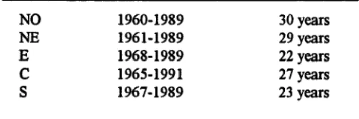
The number of years available for the analysis is shown in Table 5.1. The fact that the series are relatively short explains much of the fluctuations in the observed periodic statistics.

NO NE

E

C S

Table 5.1 Length of data series

1960-1989 1961-1989 1968-1989 1965-1991 1967-1989 30 years 29 years 22 years 27 years 23 years

5 Results of single-site estimation 19

Results of the fitting of three PARMA-models, PARMA(l,l), PARMA(2,1), and P ARMA(2,2) with the method of least squares (program CSU5) are presented in Appendix C. The periodic autocorrelation structure of each model has been computed according to the algorithrn described in Chapter 2 (the MATLAB code is presented in Appendix B). A series of figures were prepared, each corresponding to a given lagged periodic week-to-week correlation. More specificaIly, we considered the variance, and the lagged correlations of order 1, 2, 3, 4, 5, and 10. When comparing the three PARMA models Most attention was given to the variance, followed by the lag 1 week-to-week correlation, followed by the lag 2, and so forth. Furthermore, we paid special attention to the statistical properties during the flood season, since badly represented statistics during this period May result in flood scenarios that deviate significantly from the historical (in an average sense).

5.2 North East region

From the figures

in

Appendix Cl, it is seen that the PARMA(l,l) preserves the variance of the transformed, standardized flows very weIl. In the first few periods it deviates from 1, probably due to the initialization of the first residual in the LS-estimation algorithrn. The variance ofboth PARMA(2,1) and PARMA(2,2) deviates significantly from 1. Deviations of 20-25% are observed in some periods. In the critical flood season (week 26-35) the PARMA(2,2) seems to deviate more than the PARMA(2,1) from 1. For correlations up to lag 4, PARMA(2,1) and PARMA(2,2) do weIl, whereas the PARMA(I,I) does not satisfactorily described the critical correlations during the flood season. The P ARMA(2, 1) seems to do slightly better than the P ARMA(2,2) in describing the lagged correlation. The PARMA(2,1)-model was therefore selected as the Most adequate model for the North East region.

5.3 North West region

For the North West region, the variance is best reproduced by the PARMA(I,I)-model. The P ARMA(2,2) generally does a better job than the P ARMA(2, 1) in reproducing the periodic variance, and notably in the critical flood season. As for the lagged correlations, the P ARMA( 1,1) fails to reproduce satisfactorily the correlations during the flood periods, whereas the other two models essentially do equally weIl. In the light of these observations, it was decided to choose the PARMA(2,2)-model for the North West region.

5.4 East region

Again the PARMA(l,l) preserves the variance almost exactly. The PARMA(2,l) and P ARMA(2,2) fluctuates quite much and seem to be equally good (or bad). The same thing can be said about the lagged correlations, where there is little difference between the two. The PARMA(I,l) aIso here fails to reproduce the negative correlations during the flood season. Since the two higher order models yield quite similar results, the P ARMA(2,l)-model is selected in accordance with the principle of parameter parsimony.

5.5 Central region

For the Central region, the variance of the PARMA(2,2) deviates up to 70% from the historical, transformed variance during severai weeks around and following the flood season, and it was therefore excluded. Both P ARMA(l,l) and P ARMA(2,l) do a good job in describing the variance and the lagged correlations, although for the last property, the P ARMA(2, 1) seems slightly superior. It is therefore selected as the appropriate model.

5.6 South region

Historical statistics for the South region are characterized by large fluctuations. The P ARMA(2,2) yields a relatively poor representation of the variance of the transformed process, the PARMA(l,l) does excellently, and the PARMA(2,1) is somewhere in between. As for the lagged correlations, the PARMA(2,2) seems worst, the PARMA(1,l) seems better, and the PARMA(2,1) seems best, although the difference between PARMA(l,l) and PARMA(2,1) is small. As a whole, it seems that the PARMA(l,l) provides a reasonable description of the data for the South region.

5.7 Summary of results

5 Results of single-site estimation 21

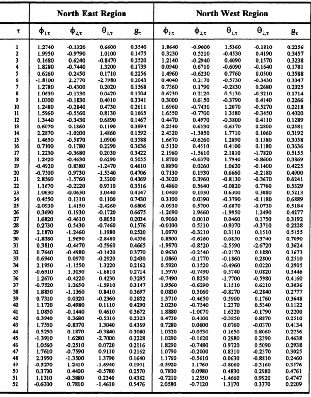
Table 5.2 Estimated P ARMA(p,q)-parameters for the five regions in the Ottawa River.

North East Region North West Region

or _{cl>1.'t cIl2.'t}

₉

_{1.'t g't cIlI.'t cIl 2.'t}

₉

_1.'t

₉

_{2.'t gt}

1 1.2740 .0.1320 0.6600 0.3540 1.8640 .0.9000 1.S360 -0.1810 0.2256 2 1.9950 .0.9790 1.0100 0.l475 0.3230 0.5210 -0.4530 0.4190 0.3457 3 0.1680 0.6240 .0.8470 0.2520 1.2140 -0.2940 0.4090 0.1570 0.3238 4 1.8280 .0.7440 1.3200 0.1739 0.0940 0.6710 .0.6090 -0.1640 0.1781 5 0.6260 0.2450 0.1710 0.2256 1.4960 -0.6230 0.7760 0.0500 0.3588 6 -1.8100 2.2770 -2.7980 0.2043 0.4040 0.2170 -0.5730 -0.3430 0.3047 7 1.2780 .0.4300 0.2020 0.1568 0.7360 0.1790 -0.2830 0.2680 0.2025 8 1.0630 .0.1330 0.0420 0.1204 0.6230 0.2120 0.5130 -0.3210 0.1714 9 1.0300 .0.1830 0.4010 0.3341 0.3000 0.6150 .0.3790 0.4140 0.2266 10 1.2480 .0.2840 0.4730 0.2611 1.6960 -0.7430 1.2070 -0.5270 0.2218 11 1.5960 .0.5560 0.8130 0.l665 1.6550 -0.7700 1.3580 -0.3450 0.4020 12 1.3440 .0.3430 0.6890 0.1467 0.4470 0.4970 -0.3800 0.4110 0.1289 13 0.6070 0.1860 0.1190 0.3994 0.2540 0.6530 -0.6570 0.2800 0.2581 14 2.2870 -1.0200 1.4860 0.1592 2.4320 -1.3050 1.7710 0.1060 0.3192 15 1.4650 .0.5870 1.0900 0.3588 1.6670 -0.6260 1.2890 0.1580 0.3058 16 0.7100 0.1780 0.2290 0.3636 0.5130 0.4510 0.4100 0.1180 0.3636 17 1.2230 -0.3680 0.2030 0.3422 2.1960 -I.S610 2.1810 -1.7820 0.5155 18 1.2420 .0.4630 0.6290 0.5055 1.8700 .0.6370 1.7940 -0.8600 0.3869 19 -0.4920 0.8380 -1.2470 0.4610 0.8890 0.0260 1.0620 -0.1400 0.4225 20 -0.7500 0.9730 -U340 0.4706 0.7130 0.1930 0.6660 -0.2180 0.4900 21 2.8560 -1.S760 2.5200 0.4369 -0.3020 0.3960 .0.8130 -0.3670 0.6241 22 1.1670 .0.2220 0.9310 0.3516 0.4860 0.5640 .0.0820 0.7760 0.5329 23 1.0630 .0.0630 1.0440 0.4147 1.0400 0.1030 0.6300 0.3080 0.5213 24 0.4550 0.1310 0.1100 0.7430 0.3100 0.0390 .0.3790 -0.1180 0.6889 25 -2.0930 1.4150 -2.4260 0.6806 -0.0930 0.5700 .0.6070 -0.0730 0.5184 26 0.3690 0.1930 .0.1720 0.6675 -1.2690 1.9660 -1.9950 1.2490 0.4277 27 1.6820 -0.4610 0.8050 0.2034 0.9060 0.0010 0.0460 0.1750 0.3192 28 0.2730 0.5430 .0.7460 0.1576 -0.0100 0.5310 .0.9370 -0.3710 0.2228 29 2.1870 -1.2460 1.1980 0.2520 1.0970 .0.3210 0.3110 0.ISI0 0.5155 30 -1.8380 1.9690 -2.8480 0.4556 0.8900 .0.6260 0.0850 0.3740 0.7090 31 0.3810 -0.4470 .0.5960 0.4665 -1.9970 .0.8520 -2.5590 -2.6720 0.3624 32 0.7640 -0.4980 -0.1420 0.3770 0.9630 -0.2540 -0.2170 0.1880 0.1673 33 0.6940 0.0970 -0.2920 0.2430 1.0860 -0.1770 .0.1860 0.2800 0.2510 34 2.1950 -1.1550 1.3220 0.2162 0.5920 0.1520 -0.4960 0.0220 0.2905 35 -0.6910 1.3030 -1.6810 0.2714 1.S970 -0.7490 0.5740 0.0820 0.3446 36 1.2670 -0.4220 0.4230 0.3295 -0.7490 0.8250 -1.7700 -0.5980 0.4160 37 -0.7520 1.2650 -U910 0.3147 1.9560 -0.6290 1.1510 0.6210 0.3036 38 1.8850 -1.1360 0.8410 0.3697 0.0830 0.5060 .0.8270 -0.2840 0.2777 39 0.7310 0.0320 -0.2360 0.2852 1.3710 .0.4650 0.5900 0.1760 0.3648 40 1.1720 -0.4980 0.1110 0.4290 2.0230 .0.7540 1.2370 0.5340 0.1122 41 1.0850 -0.1440 0.4610 0.3672 1.8880 -1.0070 1.6320 -0.1790 0.2200 42 0.3940 0.3680 .0.5310 0.2323 0.4730 0.4100 .0.3850 0.8870 0.2510 43 1.7550 -0.8370 1.3040 0.4369 0.7280 0.0600 0.0760 -0.0370 0.4134 44 0.5250 0.1870 .0.3840 0.3080 1.0320 .0.0530 0.1650 0.8060 0.2256 45 -1.3910 1.6280 -2.7000 0.2228 1.0290 -0.1620 0.2980 0.2390 0.4638 46 1.0560 -0.2510 0.0720 0.2116 1.8290 -0.7480 0.9720 0.5090 0.2938 47 1.7610 -0.7590 0.9110 0.2162 1.0790 -0.2000 0.8310 -0.2370 0.3025 48 2.3950 -1.3500 1.3790 0.1640 1.1760 -0.5610 0.0630 -0.8810 0.2460 49 .0.5270 1.2410 -1.6940 0.l901 -0.5920 1.1760 -0.8060 -0.3160 0.3576 50 0.3700 0.4400 .0.5780 0.2570 0.7830 0.0980 0.4830 0.2980 0.4761 51 1.1310 -0.3880 0.2340 0.4382 -0.7210 1.2550 -1.4660 0.9920 0.4747 52 -0.6300 0.7810 -1.4610 0.5476 2.0580 -0.7120 1.3170 0.3370 0.2209

Table 5.2.(cont.)

East Region Central Region

't cj)I,'t cj)2,'t

9

1,'t g't cj)I,'t cj)2,'t

9

1,'t g't 1 -1.9750 2.1270 -3.0740 0.1163 0.5000 0.3470 -0.1400 0.4330 2 0.6650 0.1160 -0.3930 0.2107 2.4540 -1.3140 U630 0.1260 3 4.4630 -2.8420 3.6180 0.0918 0.1610 0.6950 -0.5550 0.2247 4 1.4070 -0.4400 1.7340 0.0900 0.5520 0.3590 -0.2150 0.1665 5 0.4990 0.3200 -1.2600 0.0497 U160 -0.6310 0.7850 0.3283 6 0.2780 0.5660 -2.4530 0.0488 0.4430 0.3390 -0.4900 0.2209 7 0.8710 0.0540 0.7700 0.0876 0.7420 0.0120 -0.4020 0.2652 8 1.1740 -0.3240 0.2140 0.1731 0.9490 -0.0670 -0.0950 0.2470 9 0.8890 0.0300 0.3750 0.2581 -0.5130 1.1300 -1.1950 0.4970 10 2.1450 -1.0870 1.1580 0.1849 -0.5800 1.0500 -1.4370 0.2294 11 1.4560 -0.5140 0.7030 0.2007 0.2920 0.4990 -0.7190 0.1927 12 1.4490 -0.4320 0.7050 0.1764 2.3620 -1.2790 U980 0.0986 13 2.9620 -1.7580 2.6810 0.1714 1.8950 -0.9100 1.2010 0.1414 14 0.6360 0.2970 -0.5390 0.1267 -0.2170 1.0850 -1.3180 0.0784 15 0.9410 -0.0440 0.5470 0.0955 U110 -0.5660 1.0970 0.1858 16 2.0060 -1.0040 1.1750 0.0930 1.1940 -0.1670 1.4140 0.1011 17 0.1870 0.5880 -0.6000 0.1376 0.6060 0.2870 0.5810 0.3192 18 1.4540 -0.5150 0.6250 0.1884 0.6860 0.2420 0.6030 0.3600 19 1.1300 -0.2250 0.3060 0.1731 0.3130 0.5170 -0.0010 0.4147 20 2.3280 -1.2420 1.6000 0.2343 0.6000 0.4590 0.5030 0.2088 21 2.7280 -U64O 1.9080 0.2652 0.6390 -0.0530 -0.4200 0.4886 22 2.1520 -1.1630 1.1570 0.2052 0.8290 0.1330 0.0910 0.2218 23 -0.4440 1.1570 -1.4780 0.1945 0.2370 0.4630 -0.3670 0.4610 24 0.2740 0.5120 . -0.7550 0.2480 2.6180 -1.3040 2.2120 0.5155 25 -0.3830 1.0740 -1.4400 0.2079 -0.0680 0.5380 -0.7070 0.5402 26 -1.9280 2.1240 -3.0710 0.4045 0.9360 -0.2790 0.2250 0.5730 27 0.4590 0.1020 -0.6940 0.2642 -0.0680 0.5430 -0.8320 0.4122 28 0.1910 0.5810 -0.8370 0.1498 -0.0420 0.6060 -0.9570 0.3318 29 -0.2730 0.7260 -1.6330 0.5685 -0.8650 1.1980 -1.8200 0.4343 30 -0.4810 0.0940 -U310 0.2162 1.6920 -1.6320 1.0990 0.5170 31 1.1360 -0.6510 1.1810 0.1697 0.8900 -0.1990 0.2980 0.2460 32 0.7310 -0.1160 -0.6960 0.3352 1.8890 -0.9950 0.8690 0.2992 33 1.8900 -0.9240 0.9350 0.2061 0.7180 0.0520 0.2680 0.4212 34 0.5980 0.1690 -0.3970 0.3844 -0.4560 0.8500 -1.3030 0.3147 35 1.7940 -0.7420 0.8730 0.2621 2.1100 -1.1340 1.4110 0.3411 36 U600 -0.6910 0.5920 0.1962 -0.1350 0.7040 -0.9200 0.4462 37 2.3640 -1.3000 1.5360 0.1608 -0.2890 0.6450 -1.1110 0.4970 38 1.4680 -0.5420 0.8670 0.2352 1.4100 -0.3820 0.9010 0.4238 39 -0.2020 0.7060 -1.4990 0.1772 -0.1100 0.6590 -1.1220 0.2190 40 0.6410 0.1990 -0.4180 0.3329 1.1350 -0.1400 0.5630 0.1798 41 2.8380 -1.6420 2.0100 0.1739 0.6070 0.1620 -0.7600 0.1608 42 3.0950 -2.2010 2.6300 0.2401 0.1420 0.6020 -1.1580 0.1980 43 1.1230 -0.1100 0.1980 0.2025 1.0570 -0.0790 0.6830 0.2125 44 -0.4660 1.2140 -1.2820 0.3469 1.0140 -0.2000 0.0100 0.2970 45 0.8170 1.2050 -1.8580 0.3399 -0.2190 0.8660 -1.3040 0.1832 46 1.4630 -0.5730 0.7610 0.3147 U460 -0.5920 1.2010 0.3114 47 U270 -0.3680 0.4920 0.0918 1.0710 -0.1550 0.2960 0.2621 48 -0.2240 1.1730 -1.2030 0.1529 0.7100 0.1660 0.2710 0.3434 49 -1.0500 1.8210 -1.9740 0.1190 0.2280 0.4830 -0.6110 0.3272 50 U130 -0.7440 0.7730 0.3795 -1.1070 U130 -2.2340 0.1648 51 2.1140 -0.9100 1.3840 0.2125 0.9030 -0.0630 0.0280 0.2894 52 -1.1180 1.5980 -1.9900 0.2992 0.8010 0.0590 0.4150 0.4160

5 Results of single-site estimation 23 Table 5.2 (cont.) South Region 't <l>l,'r

8

1't g't 1 1.1110 1.2380 0.5198 2 0.8170 0.7010 0.6740 3 0.7140 0.4110 0.7868 4 1.4450 1.2860 0.4872 5 1.1360 1.1620 0.3660 6 0.8740 0.1750 0.3352 7 0.7080 -0.0600 0.4692 8 0.7770 0.1060 0.4556 9 0.8050 0.7070 0.6593 10 0.9790 1.0340 0.6577 11 1.1580 0.6950 0.4007 12 0.9120 0.4740 0.4212 13 1.0920 1.1400 0.3215 14 0.8590 0.6750 0.4844 15 0.8920 0.3430 0.4449 16 0.5570 0.1240 0.7482 17 1.4960 1.2400 0.3709 18 0.8700 0.5250 0.4858 19 0.9780 0.5210 0.4083 20 0.6570 0.3950 0.7140 21 0.6370 -0.0610 0.5213 22 0.6530 0.2920 0.7586 23 0.7940 0.8830 0.8263 24 -0.6750 -1.2580 0.6320 25 0.3980 -0.4220 0.5285 26 -0.1520 -0.9990 0.6006 27 0.0380 -0.9440 0.4238 28 0.4300 0.2850 0.8855 29 -1.3940 -1.9750 0.4720 30 0.8810 0.5730 0.5491 31 0.5490 0.4920 0.8668 32 1.4410 1.0130 0.5550 33 0.7750 0.2540 0.5883 34 0.8260 0.4300 0.6194 35 0.4030 -0.3610 0.5746 36 0.2760 0.0500 0.9235 37 2.1880 2.2490 0.7174 38 0.5440 0.0760 0.7621 39 0.7670 0.5300 0.8154 40 -0.1640 0.0200 1.0302 41 ..0.6480 -0.9100 0.8336 42 1.9550 2.0170 0.6593 43 0.6060 0.4160 0.8.446 44 1.4030 1.6030 0.6496 45 1.0910 0.9820 0.5868 46 1.0090 0.8660 0.5776 47 0.4930 0.2570 0.8668 48 l.S160 1.4880 0.6839 49 0.7850 0.5150 0.7500 50 0.7490 0.8150 0.8464 51 1.1180 0.7850 0.7379 52 1.1890 1.1370 0.6257

6

ESTIMATION OF THE CROSS-COVARIANCE

OF RESIDUALS

6.1 Introduction

In order to generate flow sequences that are coherent in space, a multivariate model must be formulated. Due to the complexity of parameter estimation, the parameter matrices given in (1) are rarely considered full. An exception is the multivariate PAR(p)-model ofMatalas (1967), which, however, is deemed inadequate for the present study. A common approach is to consider the parameter matrices c})i,'f and 9~'f diagonal. This procedure is denoted contemporaneous modeling, because only the lag-O cross-correlation of (transformed) flows can be explicitly modeled through the spatial covariance of the residuals. By considering the parameter matrices diagonal, the different sites involved in the analysis are decoupled and can be studied separately. Hence, when the parameters at each site have been estimated, only the spatial correlations of residuals remain to be determined.

In this section, we address the question of how to estimate the spatial correlation of residuals. There are essentially two possible avenues: the method of maximum likelihood and the method of moments. The former is by far the most used for more complicated seasonal models. It consists in deriving the residual series of each site and then to compute the correlation matrix for each season from these series. The ML method is thus easy to implement, and always yields results, but it tends to underestimate the true correlations. Stedinger et al. (1985) derived the moment estimator of the covariance matrix in the case of a contemporaneous stationary ARMA(I,I) model, and specifically conclude that for multivariate annual ARMA(I, 1) models, the estimator of the residual covariance matrix that reproduces the observed correlation generally is superior to the maximum likelihood estimator.

Haltiner and Salas (1988) extended Stedinger results to the contemporaneous PARMA(I,I) case. Their derivation of the estimator of G'f (periodic cross-covariance matrix of the

residuals) is instructive and is briefly reviewed here. By squaring the left and the right hand sides of(I), with p

=

q

=

1, one obtains

(5)

where the year index has been omitted for notational convenience. i't and ê't are assumed known. Noting that E[SST]

=

G't' E[x't_IE!]

=

0, and E[E'tE!_I]

=

0, the above relation can be written:

(6)

in which only the G't-matrices are unknown. Note that G't depends on G't_1 etc. If a feasible solution to (6) exists, then the model will exactly reproduce the variance of the (transformed) flows at each site. However, there is a potential risk in combining, for example, LS-estimators of the autoregressive and moving average parameters with moment estimators of the residual variances. The combined solution may not be coherent and could at sorne sites lead to periodic autocorrelations that deviate more trom the observed correlations than the pure LS-estimation. It then becomes particularly important to compute each sites periodic auto correlation as described previously. If the solution to (6) is unsatisfactory, one can choose to preserve only the cross-covariances between sites exactly, i.e. the off-diagonal elements of M't(O). The procedure for doing this will be described later. In the following, we consider the problem of estimating G't by the method of moments when the individu al site models are PARMA(2,2), or, in general, any submodel hereof.

The derivation of (6) is fairly straightforward, because G't can be easily expressed (although implicitly) as a function of the properties to be preserved, M't(O). In the case of the contemporaneous PARMA(2,2) model, the derivation of a G't-estimator is less evident. Note that if the left and right hand site of(I), with p = q = 2 are squared, then lagged cross-correlations will appear. However, contemporaneous P ARMA models do not permit to preserve explicitly lagged cross-correlations. Preservation of the symmetric M't(O) matrices imposes com(m

+

1)/2 constraints which is exactly the number of degrees of freedom in the co G't matrices. Therefore, Haltiner and Salas' results for the contemporaneous PARMA(l,l) model are not generally applicable to models ofhigher order. In the present

6 Estimation of cross-covariance of residuals

27

study, we have developed a moment estimation method for any P ARMA(p,q) model with max{p,q} ~2.

6.2 Moment estimation of spatial correlations

To estimate G't' we shall make use of the periodic multivariate Yule-Walker equations. The foUowing definition is important:

(7)

where T indicates a transposed vector or matrix. Note that M't(l) will in general not be symmetric. With these definitions, one can deduce the first three multivariate periodic Yule-Walker equations (Appendix A):

M't(O) = E[x'txn =M't(l)

è»~'t

+M't(2)

è»~.'t

+G't -[è»I.'t

-81.'t]G't_18~'t

-

[~I.'tè»I.'t-l

-è»1.'t8 1.'t_1 +è»2.'t

-82.'t]G't-28~.'t

M; (1) = E[ X't_lX;] = M't_l (0) è»~'t + M't-l (1) ~~.'t - G't_18~'t -

[~l.'t-l

- 8 1.'t-l]G't-28 i.'t (Sa) (Sb) (Sc)

A careful inspection of these equations shows that the relations corresponding to the diagonal elements are simply the univariate cases given in (3a-c). On the other hand, the off-diagonal elements of M't(O), M't(l), and M't(2), as expressed in the ab ove equations, are defined in terms of off-diagonal elements of themselves and off-diagonal elements of G't' but do not involve any terms from the diagonal of these matrices. This important observation implies that the variance terms of G't' i.e. the diagonal elements can be estimated one at the time, and the covariances, i.e. off-diagonal elements can be estimated independently of the variances. Moreover, when estimating the correlations of residuals, one needs only consider two sites at the time, since other sites do not affect the particular element in G't that corresponds to the two sites. Hence, in the following we develop the estimation procedure for two sites.

First, equation (8c) is used to eliminate Mt (2) from (8a). Then the equations corresponding to the off-diagonal elements of Mt(O) and Mt(1) are written out. Considering first the entry (1,2), we obtain trom (8a-b)

_[(~(1)~(1) _ ~(l)Ô(1) + ~(1) _ Ô(l) )Ô(2) + Ô(l) ~(2)] G(12) _ (~(1) _ Ô(1»)Ô(2) G(12) l,t l,t-1 l,t 1;t-1 2,t 2,t 2,t 2,t 2,t t-2 l,t l,t l,t t-l (9a) +G(12) + ~(1)~(2) M(12) (1) + l(2) M(12)(1) = M(12) (0) _ ~(1)~(2) M(12)(0) t l,t 2,t 't-1 'Vl,t 't 't 2,'t 2,t t-2 (9b)

The IN is used here to distinguish known terms, either estimated parameters or moments

calculated trom the data, trom the terms which are to be estimated at this step. Hence, there is an important difference between, for example, M~12) (0) and M~12) (1). The former is estimated trom the data and preserved by the model; the latter is a model property, not necessarily equal to what one would get by estimating it from the data. G~12) is the covariance between the residuals at time t, and M~12)(O) = M~21)(O) is the cross-covariance of lag zero, estimated from the data. Since the data are assumed standardized, the cross-covariance is equal to the cross-correlation. The lag 1 cross-cross-covariance is defined as

M~12)(1) = E[X~l)X~:>d. It is important to note that in general M~12)(1)::t: M~21)(1). The above expressions have been obtained trom (8a-b) by considering the element (1,2). Two other sets of equations can be obtained by considering the elements (2,1) in (8a-b), which corresponds to switching the site indices in (9a-b). Note that the element G~12) remains unaltered, since G~12) = G~21). Renee, we essentially have 4ro linear equations with 3ro unknowns, namely G~12), M~12)(1), and M~21)(1) for t

=

1, .. ,ro . In fact, one of the sets of

equations is superfluous, and can be omitted. Eventually, it can be used to check the solution. Renee, we consider the system of linear equations consisting of (8a-b) and (Sb) with reversed site indices. These 3ro equations can without any major difficulty be solved for

G~12), M~12)(1), and M~21)(1).

If the variance of the flows at each site is not preserved exactly by the individual univariate models, then M~12)(O) on the right side of the above equations must be adjusted with a factor

~M~l(O)

M;Z(O) where the terms in the square root are the variances produced by

the individual models. This adjustment is necessary in order to correctly reproduce the correlation of flows.

6 Estimation of cross-covariance of residuals 29

The complex structure of the individu al site models may impose such constraints on each series that exact preservation of the spatial cross-correlation of flows is not feasible. For example, it may appear that sorne of the estimated correlations between residuals are greater than one or less than minus one. This, of course, is meaningless, and sorne adjustment of the estimated G't-matrices is needed. In general, the requirement to the G't matrices is that they be positive semidefinite. Hence, if a given G't matrix is negative definite, an adjustment must be made to make it positive semidefinite. Generally, this will imply that the correlation of flows will no longer be exactly preserved. The adjustment should have as titde influence on the G't matrices as possible. There seems to be no standard method for adjusting symmetric, negative definite matrices so as to make them positive semidefinite. If a G't matrix is negative definite (i. e. have negative eigenvalues) then one could proceed as follows:

1) Decompose the G matrix in eigenvectors and eigenvalues, P and A, where the columns of P contain the eigenvectors of G, and A is a diagonal matrix with the eigenvalues on the diagonal. Hence, G

=

PAPI.

2) Set the negative eigenvalue in A equal to zero. This defines a new matrix A*. 3) Compute the matrix G*

=

PA* Pl, which is positive semi-definite.

4) In order to preserve the variance terms of the original G matrix (i.e. the diagonal elements), perform the following computation

Gadj =UG*U where U=

o

o

o

o

o

In order to check to what degree the cross-covariance of the transformed flows are reproduced by the obtained estimates of G~12), equations (Sa-b) (with M't(2) eliminated from (Sa) by means of(Sc» are reformulated as a system of4oo linear equations in M~12)(O),

_~(1)~(2) M(12)(0)+M(12)(0)_~(I),k(2) M(12)(I)_,k(2) M(12)(1) 2,'t 2,'t 't-2 't 1,'t'l'2,'t 't-I 'l'I,'t 't

= -ê(1) Ô(12)~(2) + Ô(12) _ (~(1) _ ê(1»)Ô(12)ê(2)

2,'t 't-2 2,'t 't I,'t l," ,,-1 I,'t (10a)

_(~(1)~(1) -~(1)ê(1) +,k(I) -ê(I))Ô(12)ê(2)

l," 1,"-1 l," 1,,,-1 '1'2," 2," ,,-2 2,"

,k(2) M(2) (0) + i(2) M(12) (1) - M(21) (1) = Ô(12)ê(2) + (i(1) - ê(1) )Ô(12)ê(2) (lOb)

'l'l," 't-I 'l'2,'t ,,-1 " ,,-1 l," 'l'I,'t-1 1,,,-1 ,,-2 2,'t

plus the same two sets of equations with reversed site indices. Strictly, only three equations are needed, since M~l2) (0) = M~21) (0). However, the above formulation provides a test of coherence. In a fi.rst step, one should verify that M~12)(0) is identical to M~21)(0). Ifnot, this could indicate a programming error or lack of precision in the computation. The model cross-covariance M~12)(0) can be compared with the observed cross-covariance of the transformed data M~12)(0).

Lagged cross-correlations are not preserved explicitly. The extent to which an estimated model produces lagged cross-correlations that resembles the observed can be examined by comparing M't(l) and M't(2) of the model with the corresponding observed lagged cross-covariance matrices. Note that M,,(l) is obtained as a biproduct in the estimation of G't' With known M,,(O) and M't(l), M,,(2) is readily obtained from (Sc). One can generalize equation (3d) to the multivariate case:

M,,(k) =

E[X"X;_k]

= Cl»1." M"_I(k-l) + Cl»2,,, M't-2 (k-2) k>2 (11) but usually only the first or second lagged correlations need to be examined.

7

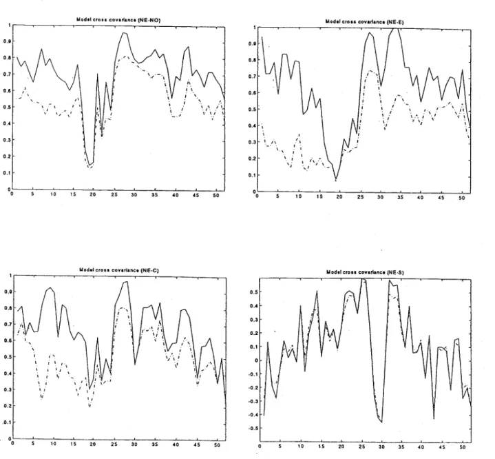
RESULTS OF MULTI-SITE ESTIMATION

The method of moments was used to estimate the off-diagonal elements of the periodic cross-covariance matrices of residuals. The MATLAB computer codes used to compute these properties are presented in Appendix B. The G'f-matrices have dimension 5x5, but only 10 elements in each are unknown, corresponding to the number of combinations of two sites out of five. Estimated autoregressive and moving average parameters of each pair of sites, as weIl as the observed periodic cross-correlation of transformed flows, were entered into a program, which as output yielded the periodic cross-covariance of residuals needed to reproduce the cross-correlations of flows. This resulted in ten vectors of periodic cross-covariances of residuals, representing an initial estimate of the ten off-diagonal elements of the G'f -matrices. As noted in the previous section, there is no guarantee that this is a feasible solution. The G'f -matrices must be positive semidefinite, but there is no provision for this in the method of moments. In fact, the problem pertaining to negative detinite matrices turned out to be more severe than expected. Only one of the 52 matrices were positive definite, 21 matrices had one negative eigenvalue, 28 had two negative eigenvalues, and two had three negative eigenvalues. Ali matrices with negative eigenvalues were modified with the technique described in the previous section. This had a significant effect on sorne of the elements of the matrices. The matrix G 1 had three negative eigenvalues, G₂ had two negative eigenvalues, and G₃ had one negative eigenvalue. The first three G-matrices were changed as follows2 :

[""

0.49 0.70

"53

~~I

0.35 0.28 0.20 0.38

~31

0.23 0.88 0.63 -0.45 0.23 0.16 0.31 -0.24 °1= 0.12 0.79 -0.25 0'-\ - 0.12 0.22 -0.15 0.43 -0.35 0.43 -0.29 0.52 0.52 0.15 0.11 -0.14 0.00 0.17 0.15 0.10 -0.04 0.04 0.10 0.35 -0.23 0.24 0.12 0.35 -0.15 0.20 0.10 0,= 0.21 -0.23 0.45 G'-

.-

0.21 -0.08 0.25 0.13 0.13 0.13 0.06 0.67 0.67

2) The elements of the matrices correspond to the regions in the following order: North East, North West,

Table 7.1 Elements of the periodic covariance matrices ofresiduals 1 gl1 g12 g13 g14 g15 g22 g23 g24 1 0.3540 0.2819 0.1983 0.3844 ..().3204 0.2256 0.1604 0.3104 2 0.1475 0.1047 ..().0418 0.0357 0.1041 0.3457 -0.1538 0.2035 3 0.2520 0.2643 ..().0939 0.1330 ..o. 1907 0.3238 -0.1158 0.1726 4 0.1739 0.1243 ..().0828 0.1308 ..o. 1998 0.1781 ..o. 1066 0.1279 5 0.2256 0.1637 0.0511 0.1373 ..().0928 0.3588 0.0997 0.2250 6 0.2043 0.0737 0.0322 ..0.0602 0.1127 0.3047 ..().0843 0.1700 7 0.1568 0.1043 0.0818 0.0313 ..().0207 0.2025 ..().0189 0.1924 8 0.1204 0.0891 0.0087 0.1350 0.0634 0.1714 -0.1255 0.1965 9 0.3341 0.1797 0.1806 0.3385 ..().0497 0.2266 0.0253 0.2070 10 0.2611 0.1483 0.1206 0.1560 0.3679 0.2218 0.0120 0.0579 11 0.1665 0.0998 -0.1170 ..().0437 ..o. 1495 0.4020 ..().0716 0.0803 12 0.1467 0.0800 ..().0575 0.1137 0.1331 0.1289 0.0257 0.0593 13 0.3994 0.1710 0.0253 0.1468 0.2901 0.2581 ..().0384 0.0827 14 0.1592 0.0777 ..().0231 ..().OO44 0.2548 0.3192 0.1274 0.0933 15 0.3588 0.2497 0.0655 0.1050 ..().0952 0.3058 ..().0151 ..().0056 16 0.3636 0.2921 0.0097 0.0231 0.2039 0.3636 0.0452 0.0399 17 0.3422 0.2851 0.0499 0.1618 0.0004 0.5155 ..().0470 0.0020 18 0.5055 ..().OO77 0.0851 0.2432 0.1203 0.3869 0.0124 -0.0937 19 0.4610 ..().0392 ..().0423 0.0047 ..().0215 0.4225 0.0047 ..().0961 20 0.4706 0.0868 0.1353 0.1472 0.1871 0.4900 0.2834 0.0475 21 0.4369 0.5121 0.2590 0.4168 0.3277 0.6241 0.2573 0.4833 22 0.3516 0.2948 0.1994 0.2632 0.4194 0.5329 0.1558 0.2256 23 0.4147 0.4542 0.2495 0.3121 0.4338 0.5213 0.3004 0.3131 24 0.7430 0.3105 0.1525 0.2697 0.2692 0.6889 0.2722 0.3792 25 0.6806 0.4882 0.3356 0.5324 0.4302 0.5184 0.2969 0.4530 26 0.6675 0.5072 0.3969 0.5377 0.3914 0.4277 0.2611 0.3925 27 0.2034 0.2490 0.2102 0.2779 ..o. 1121 0.3192 0.2755 0.3224 28 0.1576 0.1197 0.1118 0.1740 "().3173 0.2228 0.1213 0.1870 29 0.2520 0.2706 0.2833 0.1998 ..().0884 0.5155 0.3249 0.2423 30 0.4556 0.5538 0.3039 0.4557 ..0.3235 0.7090 0.3522 0.5259 31 0.4665 0.3651 0.2642 0.1795 0.0084 0.3624 0.2444 0.2513 32 0.3770 0.1795 0.0452 0.3284 0.3886 0.1673 ..().0756 0.1871 33 0.2430 0.1785 0.1085 0.3050 0.2000 0.2510 0.2056 0.2699 34 0.2162 0.1662 0.2619 0.1525 0.2040 0.2905 0.1460 0.1854 35 0.2714 0.2403 0.0766 0.1565 ..().0142 0.3446 0.2329 0.2954 36 0.3295 0.3052 0.1473 0.3783 0.0429 0.4160 0.2357 0.3863 37 0.3147 0.2520 0.2015 0.1428 0.2755 0.3036 0.2057 0.3109 38 0.3697 0.1511 0.1803 0.1494 ..().0672 0.2777 0.1142 0.0803 39 0.2852 0.0789 0.0879 0.1997 ..().0186 0.3648 ..o. 1003 0.1103 40 0.4290 0.2127 0.1176 0.1307 0.1578 0.1122 0.0935 0.0586 41 0.3672 0.2834 0.1876 0.2311 ..o. 1522 0.2200 0.1351 0.1827 42 0.2323 0.2307 0.2010 0.1273 0.1208 0.2510 0.2374 0.1788 43 0.4369 0.4056 0.1447 0.1675 "().4186 0.4134 0.2055 0.2066 44 0.3080 0.1563 0.2114 0.0811 ..().0284 0.2256 0.2293 0.0137 45 0.2228 0.2628 0.1255 0.0141 0.0084 0.4638 0.3139 0.1815 46 0.2116 0.2288 0.1804 0.2136 0.0681 0.2938 0.1906 0.2303 47 0.2162 0.1340 0.0707 0.1538 "().2314 0.3025 0.1665 0.2743 48 0.1640 0.1064 0.0895 0.2331 0.1378 0.2460 ..().0773 0.1629 49 0.1901 0.1640 -0.0246 ..().0104 0.0435 0.3576 0.0918 0.2334 50 0.2570 0.2490 0.2624 0.1251 ..0.2266 0.4761 0.3775 0.2640 51 0.4382 0.2652 0.0296 0.3061 ..o. 1207 0.4747 0.1537 0.2712 52 0.5476 0.1644 0.1804 0.0530 ..0.3323 0.2209 ..o. 1398 0.2026