On the Construction of Confidence Intervals for the Quantiles of the Gamma Distribution.

Author Role:

Title, Monographic:

On the construction of confidence intervals for the quantiles of the

Gamma distribution

Translated Title:

Reprint Status:

Edition:

Author, Subsidiary:

Author Role:

Place of Publication:

Québec

Publisher Name:

INRS-Eau

Date of Publication:

1988

Original Publication Date:

Mai 1988

Volume Identification:

Extent of Work:

23

Packaging Method:

pages

Series Editor:

Series Editor Role:

Series Title:

INRS-Eau, Rapport de recherche

Series Volume ID: 252

Location/URL:

ISBN:

2-89146-249-1

Notes:

Rapport annuel 1987-1988

Abstract:

10.00$

Call Number:

R000252

Keywords:

rapport/ ok/ dl

CONFIDENCE INTERVALS FOR THE

QUANTI LES OF THE GAMMA DISTRIBUTION

FAHIM ASHKAR AND BERNARD BOBEE

Institut national de la recherche scientifique

(INRS-Eau)

C.P. 7 500,

Sainte-Foy, Québec, CANADA

G1V 4C7

Rapport scientifique no. 252

mai 1988

ON THE CONSTRUCTION OF CONFIDENCE INTERVALS

FOR THE QUANTI LES OF THE GAMMA DISTRIBUTION

Fahim Ashkar and Bernard Bobée

Institut national de la recherche scientifique (INRS-Eau),

C.P. 7 500, Sainte-Foy, Québec, canada GIV 4C7

We present an approximate method for constructing confidence intervals

for the quantiles of the 2-parameter gamma distribution when both scale and

shape parameters

e

and

le,

respectively, of the distribution are unknown.

There is a relationship between these confidence intervals and one-sided

tolerance limits for the distribution. Simulation shows that the method is

highly accurate for many practical applications.

The method is also quite

general and might be useful for other distributions as well.

KEYS WORDS: Confidence bounds; percentiles; tolerance limits; approximate

methods; small and moderate sample sizes; simulation.

1. INTRODUCTION

A well known problem in statistics is how to calculate a lower 'Y probability tolerance limit for proportion 1-p of a given statistical distribution. This can also be regarded as a lower 'Y level confidence limit for the pth quantile x of the distribution because if L(x

;'Y)

is a lower

'Y

p p

LeL for x and R(t) is the reliability at time t, then p

Pr { R(L(x

;'Y))

~ 1-p}

=

'Y

p

where by definition R(t)

=

1-F(t) and F(·) is the cdf of the distribution.

Ways of obtaining exact confidence limits for quantiles of such distributions as the normal/log normal, extreme value type 1 /Weibull, and exponential, are weIl known and weIl documented in the statistical literature. One distribution for which a method for constructing exact confidence limits for its quantiles is not yet known, is the gamma distribution in the case where the two parameters

e

and K of the distribution are unknown. This because unlike the other distributions mentioned above, the paramet'ers of the gamma distribution are not of the location-scale type. Approximate methods for the gamma distribution have been sought for quite a long time and it is only recently that Bain, Engelhardt and Shiue (1984) have had sorne success in developing a usefully approximate method for this distribution. The tolerance limits obtained by Bain et al. for the gamma distribution are calculated by first assuming the distribution mean known and the shape parameter (K) unknown, and then

replacing the distribution mean by the sample mean. This method is shown to be satisfactory for quite a broad range of values of the shape parameter, and for moderate sample sizes, but not for aIl probability levels p.

In fact, for values of p greater than .20, the method of Bain et al. fails to produce good results. Therefore, in situations where one is interested in constructing confidence intervals for quantiles situated at the right tail of the distribution (values of p close to unit y) , this method does not provide an adequate solution. This is exactly the kind of situation which we will be interested in, in the present study. To handle this kind of problem, we shall develop a new approximate method which we shall discuss and test using simulation. We start by presenting one area of application where quantiles of the gamma distribution play an important role.

2. DESCRIPTION OF TIIE PROBLEM

The gamma distribution (also known as the Pearson type 3 distribution) is a widely used distribution in hydrology. For example, in the area of flood frequency analysis the 3-parameter gamma distribution is very frequently used to fit annual maximum flood series which consists of the maximum discharge value recorded each year at a given gaging station over an n-year period. See Bobée (1975), United States Water Resources Council (1981) or Rao (1981) for more detail on this subject. In these references, either the annual maximum flood dis charge or its logarithm is assumed follow a 3-parameter gamma distribution.

The probability density function of the 3-parameter gamma distribution is given by:

1C-1

=

(y-n)

exp

[-(y-n)/0]

f(x;

0,IC,n)

~~~--~IC~~~L-~~~

e r(lC)

00 1C-1-t

where

r(lC)

=

Jo

t e dt is the gamma function. In the present study, we shall restrict our attention the case where the location parameter

n

is equal to zero but we mention that in flood frequency analysis

n

signifies the lower bound of flood flows and for this reason it is frequently assumed to be greater than zero (the value of

n

depends on the hydrogeographical conditions of the watershed and has to be estimated from the recorded flood sample but on certain rivers, especially those in arid or semi-arid regions

n

is sometimes taken to be equal to zero and the 2-parameter gamma distribution is obtained).

There are different ways of describing the shape of the gamma distribution one of which is by using the coefficient of skewness

r

=

2/

..;---K . The mean and variance of the gamma distribution are 2 2

respectively given by ~

=

n

+ ICS and ~

=

ICS .

X X

The design of flood control structures and other hydraulic works is usually done on the basis of a specified annual flood discharge X

T corresponding to a specified return period T (in years) where T

=

l/Pr [X ~

Xr]

is the return period of the design flood value

Xr.

In other words, if a dam is constructed to withstand the 100-year flood X

T (T

=

100), say, then the dam will be expected to be overtopped on the average once every 100 years. The probability that the dam will be overtopped in any given year will be equal to .01 (1 - p

=

Pr [ X ~

Xr ]

=

1/100

=

.01). This shows how the estimation of quantiles XT(or X

p) and the construction of confidence intervals for these quanti les comes to play an important role in hydraulic design.

This article is to present an approximate method for constructing confidence intervals for quantiles of the gamma distribution. Our method has been applied successfully to the 3-parameter gamma distribution at least for sample sizes and shape parame ter values commonly found in flood frequency analysis. From a hydrologie perspective, the method has been discussed in (Ashkar and Bobée 1987) but in the present study we shall give a brief description of the method and· apply it to the 2-parameter gamma distribution. It will be shown that for this distribution the method can give excellent results for many sample sizes (n), shape parameter values (K)

and probability levels (p) encountered in many areas of application.

3. THE PROPOSED METHOD

In equations 1 through 7 we present the method without any mathematical justification. The next two sections wil help give further clarification of the method, but it is only after Table 1 is presented, that the practical utility of the method can be fully appreciated.

Let Y be a continuous random variable with probability density function (p.d.f.) fy(Y;

el' ... , e

k), and cumulative distribution function (c.d.f.) Fy(Y;

el' ... , e

k), where

el' ... , e

k are unknown parameters. Suppose that a method exists for constructing confidence intervals for the quanti les y _p of the random variable Y. In other words, for any 100 (1 - 2~)

%

confidence level, we can calculate upper and lower confidence limits U (p) ~ and L (p) such that:

~

P [Y ~ U (p)]= ~

p ~

which implies that:

and P [Y ~ L (p)]

=

~

p ~

1 - 2~

(1)

(2)

Suppose that X is a random variable for which a method for constructing confidence intervals for X

p does not exist

FX(x; e~,

... ,

e~) be the p.d.f. and c.d.f.

Let fX(x; e~,

... ,

e~) and of X, respectively, where

e', ... , e'

are unknown parameters. What we are searching for, are two real

1 m

numbers U' (p) and L' (p) such that:

~ ~

or

p

[X

~

U'

(p)]

=

~

p ~ and p

[X

p ~

L'

~ (p)]

=

~

P [L~ (p) ~ X_p ~ U~ (p)]

=

1 - 2~

Assume for the time being that 81 , . . . , 8_k are know.n.

(3)

Let Pl be the probability of Y not exceeding L (p) and P2 the probability of it not

~ exceeding U~(p), i.e.:

P [Y ~ L (p)]

=

Pl

This means that La(p) is the pl-quantile of Y and Ua(p) is the p2-quantile of

Y:

Y

Pl

U

a (p)

=

Y

P2 (5)

If La(p) and Ua(p) are known, then Pl and P2 can be calculated using the equations:

(6)

If the c.d.f.

FX

is known, then this can be used to calculate the Pl- and P2- quanti les of

X,

namely

X

and

X

Pl P2 The method we propose consists in taking the desired lower and upper 100(1-2a)

%

confidence limits for

X

P to be equal to:

X

Pl and U~(p)

=

X P2 (7)

Before giving a mathematical justification for this approximate method we shall give an example.

4. EXAKPLE

It is weIl known that when the parent distribution of an observed sample is normal or log normal, exact confidence intervals for X can be constructed

p

as described in (Johnson and Welch, 1940). These are based on the noncentral t-distribution.

In other words, if {Y l , ... , Y } is a random sample of size n from a _n normal distribution, with mean ~ and standard deviation

a ,

then the exact

th

100 (1 - 2~)

%

confidence interval [L~ (p), U~ (p)] for the p quantile y , of Y, is given by:

p

[L~ (p), U~ (p)]

= [Y

+ SY ~~ (p),

y

+ SY ~1-~ (p)] (8)

where ~ (p) and ~1 (p) are obtained using tables of the non-central

~ -~

t-distribution (Locks, Alexander and Byars, 1973; Resnikoff and Lieberman, 1957; Odeh and Owen, 1980 and others).

The following sample, placed in increasing order, gives the maximum discharge during the month of September, over the period 1940-1966, at a gaging station on the Harricana river, Canada. The sample values are in m3_{jsec. and the sample size, n, is 27.}

19, 23, 27, 33, 39, 39, 40, 43, 50, 50, 51, 61, 62, 63, 65, 66, 71, 82, 85, 86, 89, 93, 101, 106, 117, 119, 126.

The 2- parameter gamma distribution provides a good fit to the sample, and the maximum likelihood (ML) estimates of the parameters

e

and K of this distribution (X) are respectively: ~

=

14.57 and

K

=

4.59. The estimate of the coefficient of skewness of X is therefore ~ = 2jJ 4.59 = .934 and estimates of the mean and standard deviation are ~

=

66.88 and

à

=

31.22.

x x

Suppose that we wish to construct a 90% confidence interval (~

=

0.05) for the 99th percentile of X (p

=

.99). We choose a "prior" Y to be for instance

2

choice of Y will be discussed in more detail later. From tables of the noncentral t-distribution, with n

=

27, P

=

0.99 and ex

=

0.05, we find Lex(p)

=

~ex(p)

=

1.817 and Uex(p)

=

~l-ex(P)

=

3.117, which by equation 8 are the lower and upper confidence limits for the standardized normal quantile

(Y

-~ )/cr under the assumption that

Y

=

~ and S

=

cr (we shall also

p y y y y y

return to this assumption later). The next step is to find ~ (1.817) and

~ (3.117), where ~ is the c. d. f . of the standard normal distribution. Approximation formula (26.2.17) of Zelen and Severo (1970) gives

~ (1.817)

=

Pl ~ 0.965391 and ~ (3.117)

=

P2 ~ 0.999086. From Tables of Cohen, Helm and Sugg (1969) or Tables of Harter (1964) with ~

=

.934 and non-exceedance probabilities Pl

=

0.965391 and P2

=

0.999086 we obtain the values K

~

2.13 and K

~

4.54, where K is the pth quantile of the

Pl P2 P

standardized gamma variate with coefficient of skewness ~. The values of

K

can also be calculated using program MDCHI of the Library IMSL (1982) or more conveniently by using the Wilson-Hilferty approximation (Wilson and Hilferty, 1931):

K

p

2 ~

--Our proposed method consists in taking the lower and upper confidence limits for X as follows:

p

L' (p)

u'

(p) cx and

'"

'"

=

~ +

K

a

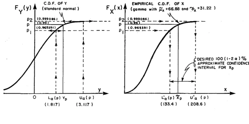
~ 208.6 x P2 x

The above numerical calculations are summarized schematically in Figure 1. What we have done, in this example, is that we have used the exact

90% confidence interval [1.817, 3.117] for the 99thpercentile of the normal distribution (Y.99)' under the assumption that Y

=

~y and Sy

=

a

_y , to construct an approxirmte 90 % confidence interval [133.4, 208.6] for the corresponding gamma percentile, X.

99, by making use of the observed sample from the gamma distribution. Had the random variable Y that we started with been Weibull, for instance, rather than normal, we would have obtained a different confidence interval for X.

99. Had Y on the other hand been lognormal or any other distribution derived from the normal by a monotonie transformation, we would have obtained exactly the same confidence interval as ab ove . We expect that the distribution Y that behaves "nearest" to the gamma distribution (X) at the probability level p, of interest, to yield the most accurate (or least inaccurate) confidence intervals for the gamma quantile X. This "best" distribution Y may vary, however, with the value

p

of the probability level p and also with the value of cx (confidence level). With the help of simulation, one can choose the best distribution Y for different values of p and cx.

We mention that for the above example the method of Bain, Engelhardt and Shiue gives L'(p) ~ 143.9 and U'(p) ~ 202.1. Had we been interested in

cx cx

a 90% confidence interval for X.

given [7.9, 22.3] while that of Bain el al. gives [7.4, 20.7]. We shall have a word to say about the two methods later.

5. MATHEHATICAL JUSTIFICATION FOR THE PROPOSED APPROACH

We know that for any two distributions X and Y, a relationship exists which gives the quanti les

X

of the distribution

X

as a function of the

p

corresponding quantiles

Y

of the distribution

Y.

This relationship is

p

given by:

(9a)

Of course, the inverse of this relationship gives

Y

as a function of p

X :

p

and both functions h(-) and h-l (-) are increasing functions.

(9b)

If FX in the last two equations is estimated by FX then h will be

'"

estimated by li and equations (9a) and (9b) will be approximate equalities rather than strict equalities_

If by using certain assumptions such as Y

=

to calculate L (p) and U (p) such that:

a. a.

1 - 20'.

=

cr we are able

y

(10)

i.e. such that [L (p), U (p)] is a 100 (1 - 20'.)

%

confidence interval for

a. a.

Y , then:

(1) taking L (p) = y and UN(p) = y as was done in (5);

a

Pl

~

P2

(2) making use of the approximate relationship Y

p ~

li-l(X

p);

and (3) using the fact that

li-l(.)

is an increasing function; we obtain:

1 - 2a

~

P [Y

~

li-

l

_{(X )}

~

_{Y ]}

Pl

P

P2

~

P [li- l (X )

~

li- l (X )

~

li- l (X )]

Pl

P

P2

~ p

(X

~

X

~

X )

Pl

P

P2

(11)

This last result means that [X ,X ] is an approximate 100 (1-2a)

%

Pl

P2

confidence interval for X , and this is basically why we suggested taking P

L'(p) = X and U'(p)= X in (7).

a

Pl

a

P2

The foregoing mathematical derivations show the logic behind the approach that we are proposing for transforming confidence intervals from one distribution (Y) to another distribution (X) but they do not tell us which distribution Y should be chosen as the "prior" for any given distribution X. This choice of Y when X is gamma distributed will be resolved by simulation, as will now be shown.

6. TESTING THE PROPOSED METHOD BY SIMULATION

Ashkar and Bobée (1987) considered the case of a 3-parameter gamma distribution (X) which is frequently used in flood frequency analysis and their study consisted of two parts:

(1) In the first part, the coefficient of skewness (shape parameter) of the variable X was assumed to be known, and i t was shown using simulation that the best distribution Y for producing confidence intervals for the quantiles of X was the n01TTK11 distribution as compared to other choices of Y such as the Weibull (2-parameter) and exponential (1- and 2-parameter). Note that when Y is taken to be 1-parameter exponential, i t is assumed that Y/Y follows the unit exponential; likewise when Y is Weibull, it is./ assumed that (Jl.n Y -Y)/ S follows the standard Extreme Value distribution.

y

(2) In the second part of the study by Ashkar and Bobée (1987), the coefficient of skewness of X was assumed to be unknown, and in this case it was shown that taking Y to be Weibull (2-parameter) gave fairly accurate confidence intervals for the quantiles of X (3-parameter gamma) for quite a wide range of sample sizes and coefficients of skewness found in practice. Of course one would presume that taking Y to be 3-parameter rather than 2-parameter Weibull would have most probably given better results, but since no simple method exists for constructing confidence intervals for

quantiles of the 3-parameter Weibull, Ashkar and Bobée did not consider this option in their study.

In what follows we shall consider the case where X is a 2-parameter gamma distribution with both parameters unknown. From exploratory simulation experiments we have observed that among the Weibull (2-parameter), normal, and exponential (1- and 2-parameter) distributions, it was the nonnal distribution that gave the best confidence intervals for quantiles X of the

p

gamma distribution. From our experience, it is not necessary to carry out a sophisticated Monte Carlo experiment in order to find out which "prior" Y is best for a given distribution X, so it was sufficient from the limited computer runs that we carried out to clearly see that the normal distribution was the best prior for the problem at hand. Although detailed results for the other distributions are not available, we mention that the normal distribution was uniformly superior to aIl other distributions that were considered (readers who are interested in comparative values of confidence intervals for the 3-parameter gamma, arrived at by normal, exponential and Weibull assumptions can refer to the paper by Ashkar and Bobée, 1987). The procedure that we propose for obtaining confidence intervals for the quanti les of the gamma distribution is therefore to take Y to be normally distributed exactly as was done in the example that we gave earlier.

We present in Table 1 the resul ts of an experiment in which 10,000 samples for each of three sample sizes n

=

10, 25, 50 were generated from the standardized gamma distribution (mean zero, variance one) with coefficient of skewness 1

=

0.2, 0.5, 0.7, 1.0, 1.5 and 2.0. For each sample size n and coefficient of skewness 1 we present the actual frequency

with which 90% and 99% confidence intervals constructed using the method proposed in the present study contained the true value of the gamma quantile

x ,

for p

=

0.002, .01, .05, .1, .5, .9, .95, .99 and .998. The exact

p

number of samples that were generated in each run (10,000) is rather subjective but we believe that it provides a good degree of accuracy. The calculation of K and K in the experiment was done using two

Pl P2

approximation formulas: the Wilson-Hilferty transformation, mentioned earlier, and the Cornish-Fisher transformation (Fisher and Cornish, 1960).

Table 1 shows that the method proposed in the present study gives very good results for a wide range of sample sizes (n), probability levels (p) and coefficients of skewness (1) of the gamma variable. Most of the frequencies reported in this table are based on the Wilson-Hilferty transformation for calculating gamma quantiles, which generally gave more reliable results-than the Cornish-Fisher transformation but a few entries in the upper right hand corner of the table are based on the Cornish-Fisher transformation. A few other entries are missing because neither transformation gave reliable results.

A comparison of Table 1 with Table 2 of Bain, Engelhardt and Shieu (1984) shows that the method proposed in the present study brings sorne clear improvements over the method of Bain et al. for values of p greater than about .20. For p < .20 one of the two methods might perform slightly better than the other, but with the computer time at our disposaI we did not find it necessary to make a detailed comparison between the two. Our main objective was to extend as much as possible the range of values of p, n and

"{ for which to test our method. For values of p lower than .20 i t is therefore le ft to the user to choose the method that he or she finds appropriate.

7. CONCLUSION

We close our discussion with the following remarks:

(1) The method proposed in the present study is general; i t remains to be seen if i t can be useful for distributions other than the 2- or 3-parameter gamma distribution;

(2) The results reported in Table 1 cover only the case where the parameters 8 and K of the gamma distribution are obtained by maximum

likelihood. The method was tested and gave approximately the same degree of accuracy when

a

and K were estimated by the method of moments, but due to lack of space, these results are not shown here;

(3) Another method which was not investigated in the present study but which the authors feel can be very useful for transforming confidence intervals from one distribution

Y

to another distribution

X

has been proposed by Stedinger (1983), and discussed in Ashkar and Bobée (1987) . The method consists in scaling confidence intervals of the quantiles Y by multiplying them by a certain factor to obtain a

p

corresponding approximate confidence interval for X , the factor being p

equal to the ratio of the asymptotic standard error of

X

to that of

y

This method was not tested because it takes considerably more p

time to program and run on a computer than the method that we have proposed

ACKNOWLEDGEMENTS

This study was made possible by grants from the Natural Sciences and Engineering Research Council of Canada (NSERC A-5797, A-8399 and strategic grant G-1617). We acknowledge the help of Marc Paradis and Louise Fortier who obtained the computer results and Claire Lortie who typed the manuscript. Acknowledgment is also due to the reviewers of an earlier version of this paper and to the edit or and an associate editor for their valuable suggestions.

REFERENCES

Ashkar. F. and Bobée, B. (1987), "Confidence Intervals for Pearson Type 3 and Log Pearson Type 3 Quantiles". Submitted to Water Resources Bulletin.

Bain, L.J., Engelhardt, M. and Shiue, W.K. (1984), "Approximate Tolerance Limits and Confidence Limits on Reliability for the Gamma Distribution". IEEE Transactions on Reliability, R-33, No. 2: 184-187. Bobée, B. (1975), "The Log Pearson Type 3 Distribution and its Application

in Hydrology". Water Resources Research, 11(5): 681-689.

Cohen, A.C., Helm, F.R. and Sugg, M. (1969), "Tables of Areas of the Standardized Pearson III Density Function".

NASA, Marshall Space Flight Center, Alabama.

Report NASA CR-61266,

Fisher, R.A. and Cornish, E.A. (1960), "The Percentile Points of Distributions Having Known Cumulants". Technometrics, 2(2): 209-225. Harter, H.L. (1964), "New Tables of the Incomplete Gamma-Function Ratio and

of Percentage Points of the Chi-Square and Beta Distributions". Aerospace Research Laboratories, Office of Aerospace Research, U. S. Air Force, 245 p.

IMSL (1982), International Mathematical and Statistical Librairies Inc. 9th edition, Sixth flood - GNB Building, 7500 Bellaire, Houston, Texas. Johnson, N.L. and Welch, B.L. (1940), " Applications of the Non-Central

T-Distribution". Biometrika, 31: 362-389.

Locks, M.O., Alexander, M.J. and Byars, B.J. (1973), "New Tables of the Non- Central T-Distribution". Aerospace Research Laboratories Report

ARL 63-19, Aeronautical Research Laboratories, Wright-Patterson Air Force Base, Ohio.

Odeh, R.E. and Owen, D.B. (1980), Tables for Normal Tolerance Limi ts , Sampling Plans and Screening. Marcel Dekker, New-York.

Rao, D.V. (1981), "Three-Parameter Probability Distributions". Journal of the Hydraulics Division., American Society of Civil Engineers, 107(HY3), 339-358, March. Process Paper 16124.

Resnikoff, G.J. and Lieberman, G.J. (1957), Tables of the Non-Central T-Distribution. Stanford University Press, Stanford, Calif.

Stedinger, J.R. (1983), "Confidence Intervals for Design Events". Journal of the Hydraulics Division, American Society of Civil Engineers, 109 (HYl), 13-27.

United States Water Resources Council (1981) , "Guidelines for Determining Flood-Flow Frequency". Bull. 17B, Hydrology Committee, Washington, D.C. September.

Wilson, E.B. and Hilferty, M.M. (1931), "The Distribution of Chi-Square". Proceedings, National Academy of Science (New York), 17(12): 684-688. Zelen, N. and Severo, N.C. (1970), "Probability Functions". Handbook of

Mathematical Functions, M. Abramowitz and 1. Stegun, eds. Applied mathematics series nO 55, U.S. National Bureau of Standards, Washington, D.C.

o

1 .... """' ... +- - - _ I -1 1

•

La (p) Y_p (1.817) I 1

•

ua( p ) (3.117 )

y

(0.965591 )

-- -

-~--t

1 1 1 'DESIRED 100 (1-2 a) % : APPROXIMATE CONE"IDENCE ,INTERVAL FOR Xp 1

x

L'Q(p)Xp u'a (p) ( 133.4 ) ( 208.6 )

FIGURE 1. Obtaining approximate confidence intervals for X using exact confidence p

intervals for X .

P The information given between parentheses corresponds to the example given in the present study.

SKh' COEF'rICIEN: or X 0.2 0.5 0.7 1.0 1.5 2.0 confi-dence n level 90S 10 89.83 90.68 90.01 90.06 89.47 _*'* 25 89.43 90.14 90.26 89.95 88.55. _*'* 50 89.87 90.00 90.48 89.49 86.2'* _*'* p • • 002 99S 10 99.03 98.98 99.03 99.17 98.94 .-25 98.88 98.80 98.95 99.12 98.83* .-50 98.95 99.05 98.90 98.96 98.36$ _*'* 90S 10 89.78. 90.47 89.77 90.02 90.55 91.48* 25 89.42 90.11 90.15 90.32 89.49 .-50 89.79 89.95 90.50 90.38 90.64 •

...

p • • 01 99~ 10 99.03 98.93 99.02 99.14 99.13 98.40 25 98.81 98.74 98.98 99.16 98.87 98.95* 50 98.93 99.02 98.94 99.07 98.58 _*'* 90S 10 89.45 89.80 89.45 89.80 90.52 90.55 25 89.38 90.11 90.27 90.13 90.82 89.93 50 89.74 90.13 90.31 90.35 90.51 88.74 p • • 05 99: 10 98.94 98.88 98.91 98.99 99.15 99.18 25 98.77 98.80 98.97 99.09 99.22 99.03 50 98.83 99.00 98.99 99.14 99.09 98.71 9O~ 10 89.4C 89.31 89.21 89.65 90.17 90.48 25 89.30 89.70 89.97 89.81 90.56 90.76 50 89.82 89.91 90.21 90.18 90.86 90.67 p •• 10 99~ 10 98.91 98.84 98.81 98.90 96.98 99.18 25 98.77 98.78 98.91 99.0C' 99.22 99.25 50 98.83 96.96 99.01 99.17 99.23 99.25 90\ 10 88.43 86.14 88.26 88.43 87.90 86.28 25 89.53 89.13 89.15 88.87 89.22 89.16 50 89.72 89.46 89.33 90.04 90.06 89.84 P • .50 99 ~ 10 98.59 98.48 98.67 98.66 98.73 98.45 25 98.92 98.71 96.96 98.54 98.70 98.75 50 98.93 98.84 98.83 98.88 99.01 98.86 90\ 10 89.09 89.28 89.25 89.58 88.62 86.72 25 89.76 89.80 89.25 89.35 89.13 89.16 50 90.05 9O.5C 90.27 89.73 89.76 89.16 P • • 90 99 \ 10 98.82 98.90 98.82 98.90 ge.83 98.93 25 99.02 99.02 98.99 98.98 98.8C ge.77 50 98.87 98.86 98.82 98.91 98.93 98.82 90\ 10 89.32 89.69 89.42 90.06 88.92 89.22 25 89.95 89.68 89.40 89.68 89.4C 89.37 50 90.11 90.37 90.40 89.90 89.81 89.09 P • .95 99 \ 10 98.90 99.03 98.92 98.97 98.86 99.00 25 99.09 99.08 99.00 99.00 98.89 98.97 50 98.93 98.88 9S.84 98.95 98.95 98.87 90\ 10 89.61 90.10 89.75 90.26 89.32 89.67 25 89.87 89.70 89.87 90.01 89.42 89.75

-

50 90.03 90.29 90.44 89.99 89.81 89.34 p • .99 99: 10 98.89 89.04 98.89 98.97 98.96 99.09 25 99.11 99.13 99.02 99.19 98.95 99.11 50 98.88 98.88 98.95 98.93 98.97 98.90 90S 10 89.85 90.26 89.97 90.32 89.53 89.82 25 89.95 89.82 89.97 90.25 89.66 89.96 50 90.08 90.20 90.47 90.06 89.83 89.39 P • • 998 99S 10 98.91 99.04 98.93 99.02 99.01 99.06 25 99.11 99.15 99.00 99.29 98.97 99.09 50 98.92 98.87 98.92 98.96 98.96 98.91 • The reported freQuenc1es Ire blSed on 10 000 si~'lted slliples for . . ch

Sillple siu n, ste. coefficient l. Ind problbility leve' p.

... These frequenci es are not reported Ncause nei ther the 1111 son-M11 ferty nor the Cornish-Fisher approxiNtion fo~l. for tllculating the qu.ntiles of the ga_ distribut10n gave reHlb'e resulu.

• These frequencin are blSed on the COMl1sh-Fisher approxiNtion fo~'"

All the orther frequencies Ire baud on the 11115on-Hilferty IPprOxiNtion fo~le.