Titre:
Title:
Semi-Analytical Method for g-Function Calculation of bore fields
with series- and parallel-connected boreholes
Auteurs:
Authors
: Massimo Cimmino
Date: 2019
Type:
Article de revue / Journal articleRéférence:
Citation
:
Cimmino, M. (2019). Semi-Analytical Method for g-Function Calculation of bore fields with series- and parallel-connected boreholes. Science and Technology for the Built Environment, 25(9), p. 1007-1022.
doi:10.1080/23744731.2019.1622937
Document en libre accès dans PolyPublie
Open Access document in PolyPublieURL de PolyPublie:
PolyPublie URL: https://publications.polymtl.ca/5503/
Version: Version finale avant publication / Accepted versionRévisé par les pairs / Refereed Conditions d’utilisation:
Terms of Use: Tous droits réservés / All rights reserved
Document publié chez l’éditeur officiel
Document issued by the official publisher
Titre de la revue:
Journal Title: Science and Technology for the Built Environment (vol. 25, no 9)
Maison d’édition:
Publisher: Taylor & Francis
URL officiel:
Official URL: https://doi.org/10.1080/23744731.2019.1622937
Mention légale:
Legal notice:
This is an Accepted Manuscript of an article published by Taylor & Francis in Science and Technology for the Built Environment on 20 June 2019, available online: http://www.tandfonline.com/10.1080/23744731.2019.1622937.
Ce fichier a été téléchargé à partir de PolyPublie, le dépôt institutionnel de Polytechnique Montréal
This file has been downloaded from PolyPublie, the institutional repository of Polytechnique Montréal
Massimo Cimmino is an assistant professor.
*Corresponding author e-mail: [email protected]
g
-Functions of bore fields with series- and parallel-connected
boreholes
MASSIMO CIMMINO
1*1Department of Mechanical Engineering, Polytechnique Montréal, Montréal, QC, Canada
A semi-analytical method for the calculation of g-functions of bore fields with mixed arrangements of series- and parallel-connected boreholes is presented. Borehole wall temperature variations are obtained from the temporal and spatial superposition of the finite line source (FLS) solution. The FLS solution is coupled to a quasi-steady-state solution of the fluid temperature profiles in the boreholes, considering the piping connections between the boreholes. The dimensionless borehole wall temperatures in the bore field and the inlet fluid temperature are obtained from the simultaneous solution of the heat transfer inside and outside the boreholes. The effective borehole wall temperature, i.e. the g-function, is defined based on the dimensionless inlet fluid temperature and a newly introduced effective bore field thermal resistance. The g-function evaluation method is validated against the DST model and its use is demonstrated in a sample simulation of a seasonal thermal energy storage system.
Introduction
The design of geothermal bore fields is facilitated by the accurate prediction of fluid and ground temperatures during their operation. The simulation of geothermal bore fields can be achieved by temporally superimposing thermal response factors, or g-functions, to obtain the fluid and ground temperature variations over the design period, e.g. 20 years or more. g-Functions are also employed in direct design methods, such as the ASHRAE method (ASHRAE 2015).
By definition, g-functions are step-response functions that give the relation between the heat extraction rate in the bore field and the effective temperature variation at the borehole walls. The g-function of a particular bore field may then be superimposed in time to obtain the effective borehole wall temperature variation due to a variable heat extraction rate in the bore field:
𝑇
𝑏∗(𝑡) = 𝑇
0−
1 2𝜋𝑘𝑠∫ 𝑄̅
′(𝑡 − 𝑡
′)
𝑑𝑔 𝑑𝑡(𝑡
′)𝑑𝑡
′ 𝑡 0(1)
where 𝑇𝑏∗ is the effective borehole wall temperature, 𝑇0 is the undisturbed ground temperature, 𝑄̅′ is the
average heat extraction rate per unit borehole length and 𝑔 is the g-function of the bore field. The effective borehole wall temperature is related to the mean fluid temperature in the bore field through the bore field thermal resistance:
𝑇̅
𝑓(𝑡) = 𝑇
𝑏∗(𝑡) − 𝑅
𝑓𝑖𝑒𝑙𝑑∗𝑄̅
′(𝑡)
(2)
where 𝑇̅𝑓 = 0.5(𝑇𝑓,𝑖𝑛+ 𝑇𝑓,𝑜𝑢𝑡) is the arithmetic mean of the inlet and outlet fluid temperature in the bore
field and 𝑅𝑓𝑖𝑒𝑙𝑑∗ is the effective bore field thermal resistance.
In fields of boreholes of equal dimensions (length and radius) with the same U-tube pipe configurations, connected in parallel and receiving evenly distributed fluid mass flow rates, the effective borehole wall temperature is typically equal to the overall average borehole wall temperature and the effective bore field thermal resistance is equal to the effective borehole thermal resistance 𝑅𝑏∗ (equal for all boreholes). Bore
fields with series connections between boreholes may feature important differences in temperature at the borehole walls and the overall average borehole wall temperature is then not representative of heat transfer between the fluid and the ground. The effective bore field thermal resistance also needs to be adjusted to account for the variation of fluid temperatures in series-connected boreholes.
The concept of g-functions was introduced by Eskilson (1987). The original g-functions were obtained numerically using a finite difference method by simulating the temperature variations at the borehole walls caused by a constant total heat extraction rate from the bore field. A condition of uniform temperature at the borehole walls, equal for all boreholes, was imposed. This condition stems from the assumptions that (i) the borehole thermal resistance is sufficiently small that the borehole wall temperature is close to the fluid temperature, and (ii) that the fluid mass flow rate is sufficiently large that the fluid temperature variations inside the boreholes are small. From these assumptions, for bore fields of parallel-connected boreholes, the borehole wall temperature is close to uniform and equal for all boreholes. For large bore fields with large amounts of boreholes, the generation of g-functions becomes computationally intensive.
Since then, analytical methods have been employed to approximate g-functions. Eskilson (1987) proposed using the finite line source (FLS) solution to approximate the thermal response of a single borehole. Zeng et al. (2002) later proposed the spatial superposition of the FLS to obtain g-functions of bore fields with
multiple boreholes. Lamarche and Beauchamp (2007a) and Claesson and Javed (2011) developed simplified formulations of the FLS solution to compute the average (over the length) borehole wall temperature. The limitation of the FLS solution is that it considers uniform heat extraction rate along the boreholes, which does not correspond to the uniform borehole wall temperature condition of Eskilson (1987) and leads to an overestimation of the g-function (Fossa 2011). The variation of heat extraction rates along the boreholes can be represented by vertically dividing the borehole into segments and modelling each of the segments with the FLS solution (Cimmino and Bernier 2014; Cimmino, Bernier, and Adams 2013; Lamarche 2017b; Cimmino 2018c), thereby respecting the condition of uniform borehole wall temperature in the calculation of g-functions. The calculation of g-functions can be accelerated by the joint use of Chebyshev polynomials or by the simultaneous evaluation of the g-functions at all times using a block matrix formulation (Dusseault, Pasquier, and Marcotte 2018). g-Functions were also evaluated numerically using the finite element method by Monzó et al. (2015) and by Naldi and Zanchini (2019). The validity of the condition of uniform borehole wall temperature was investigated by Cimmino (2015) using an FLS-based method and by Monzó et al. (2018) using a finite element method. It was found that, as the borehole thermal resistance is reduced, the borehole wall temperatures tend to uniformity.
Analytical and semi-analytical extensions of the g-functions have been proposed to extend their validity outside of pure conduction in uniform isotropic ground, and to consider short-term dynamics of the boreholes. Short-term one-dimensional radial analytical solutions that model the fluid flowing inside U-tubes as a single equivalent diameter pipe have been proposed in the works of Beier and Smith (2003), Lamarche and Beauchamp (2007b), Bandyopadhyay et al. (2008), Javed and Claesson (2011), Lamarche (2015). Line sources in composite media have been proposed by Li and Lai (2013; 2012a) to model the effect of the thermal properties of the grout material. A moving finite line source to model boreholes under the influence of groundwater flow was proposed by Molina-Giraldo et al. (2011). A finite line source solution applicable to anisotropic ground was proposed by Li and Lai (2012b). Layered subsurface properties were considered in the works of Abdelaziz et al. (2014), Hu (2017) and Erol and François (2018). Finite line source solutions for inclined boreholes were proposed in the works of Cui et al. (2006), Marcotte and Pasquier (2009) and Lamarche (2011), and were used by Lazzarotto (2016) to obtain g-functions with uniform borehole wall temperature.
The aforementioned models are only applicable to parallel-connected boreholes. Series connections between boreholes are common in borehole thermal energy storage (BTES) systems, where a temperature gradient is established in the ground for efficient charging and discharging of the storage, typically in a cylindrical volume. The most commonly used model for the simulation of BTES is the duct ground heat storage (DST) model (Pahud and Hellström 1996), which assumes that the boreholes are uniformly distributed in a cylindrical volume. The storage and fluid temperatures are obtained by the numerical solution of local and global problems. A limitation of the DST model is that the position and piping arrangement of the boreholes cannot be prescribed. A finite line source method to evaluate g-functions of fields of borehole with a mix of series and parallel connections was proposed by Marcotte and Pasquier (2014). However, their method does not consider the axial variations of heat transfer rates along the boreholes and may thus overestimate the long-term variations of borehole wall temperatures.
The objective of this paper is to obtain g-functions for fields of boreholes with a mixed arrangement of series and parallel connections between the boreholes. The heat transfer process in the bore field is divided into two regions: (1) unsteady heat conduction between the borehole wall and the surrounding ground, and (2) quasi-steady-state heat transfer between the heat carrier fluid and the borehole walls. The two regions are joined by a condition of continuity of temperature and heat transfer rate at the borehole walls. The paper expands on earlier work (Cimmino 2018b), and includes expressions to evaluate fluid temperatures and heat extraction rates in boreholes with axially varying borehole wall temperature as well as a sample simulation of a borehole thermal energy storage consisting of 144 boreholes.
The proposed method provides a contribution to the works of Marcotte and Pasquier (2014) who obtained thermal response factors of fields of series- and parallel-connected boreholes, and to the works of Cimmino (2015) and Monzó (2018) who showed the effect of the borehole thermal resistance on the long-term temperature changes in geothermal bore fields. An extension of the method of Cimmino (2016) is presented, providing simplified expressions to obtain fluid temperature and heat extraction rate profiles along geothermal boreholes. The simplified expressions, applied to series- and parallel-connected boreholes, provide a contribution to the network-based simulation methods of Lazzarotto (2014), Lamarche (2017a) and Cimmino (2018a) by reducing the size of the system of equations to be solved for the fluid and borehole wall temperatures.
Methodology
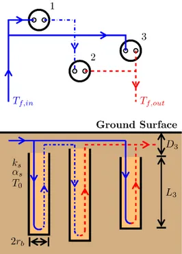
A field of 𝑁𝑏 = 3 vertical boreholes is shown on Figure 1. Each borehole 𝑖 has a length 𝐿𝑖, is buried at a
distance 𝐷𝑖 from the ground surface, and is located at coordinates (𝑥𝑖, 𝑦𝑖). All boreholes have the same radius
𝑟𝑏. Heat carrier fluid enters the bore field at a temperature 𝑇𝑓,𝑖𝑛 and leaves the bore field at a temperature
𝑇𝑓,𝑜𝑢𝑡 with a total mass flow rate 𝑚̇. The ground has a thermal conductivity 𝑘𝑠, a thermal diffusivity 𝛼𝑠 and
is initially at an undisturbed temperature 𝑇0. In the context of this paper, boreholes may be connected in a
mixed arrangement of parallel and series connections between the boreholes. Each borehole may have one or multiple U-tube pipes connected in series or in parallel. In Figure 1, boreholes 1 and 3 each receive the fluid at a temperature 𝑇𝑓,𝑖𝑛,1= 𝑇𝑓,𝑖𝑛,3= 𝑇𝑓,𝑖𝑛 corresponding to the inlet field temperature and at mass flow
rates 𝑚̇1 and 𝑚̇3 (with 𝑚̇1+ 𝑚̇3= 𝑚̇), respectively. Borehole 2 receives the fluid at a temperature 𝑇𝑓,𝑖𝑛,2=
𝑇𝑓,𝑜𝑢𝑡,1 corresponding to the outlet of borehole 1 and at a mass flow rate 𝑚̇2= 𝑚̇1 The outlet field
temperature 𝑇𝑓,𝑜𝑢𝑡 = (𝑚̇2𝑇𝑓,𝑜𝑢𝑡,2+ 𝑚̇3𝑇𝑓,𝑜𝑢𝑡,3) 𝑚̇⁄ is the result of mixing of the fluid leaving boreholes 2 and
3.
Unsteady heat conduction in the ground region
Ground temperatures in the bore field are evaluated considering heat extraction over line sources located along the axis of all of the boreholes in the field. Assuming pure conduction in semi-infinite ground with homogeneous and constant thermal properties initially at a uniform temperature 𝑇0 with the ground surface
maintained at the initial temperature 𝑇0, the borehole wall temperature along a borehole 𝑖 is obtained by the
integration of the point-source solution:
𝑇𝑏,𝑖(𝑧𝑖, 𝑡) = 𝑇0− ∑ ∫ ∫ 𝑄𝑗′(𝑧𝑗,𝑡′) 𝜌𝑠𝑐𝑠[4𝜋𝛼𝑠(𝑡−𝑡′)] 3 2 ⁄ (exp ( 𝑑𝑖𝑗2+(𝑧𝑖−𝑧𝑗)2 4𝛼𝑠(𝑡−𝑡′) ) − exp ( 𝑑𝑖𝑗2+(𝑧𝑖+𝑧𝑗)2 4𝛼𝑠(𝑡−𝑡′) )) 𝑑𝑧𝑗 𝐷𝑗+𝐿𝑗 𝐷𝑗 𝑑𝑡 ′ 𝑡 0 𝑁𝑏 𝑗=1
(3)
where 𝑑𝑖𝑗= [(𝑥𝑖− 𝑥𝑗) 2 + (𝑦𝑖− 𝑦𝑗) 2]1 2⁄ is the radial (horizontal) distance between boreholes 𝑖 and 𝑗, with 𝑑𝑖𝑖 = 𝑟𝑏,𝑖, 𝑧𝑖∈ [𝐷𝑖, 𝐷𝑖+ 𝐿𝑖] is the depth along the axis of borehole 𝑖, 𝜌𝑠 and 𝑐𝑠 are density and specific
heat capacity of the ground, 𝑇𝑏,𝑖 is the borehole wall temperature of borehole 𝑖 and 𝑄𝑗′ is the heat extraction
rate per unit borehole length of borehole 𝑗.
Following the method of Cimmino and Bernier (2014) and Cimmino (2018c), each borehole 𝑖 is divided into 𝑛𝑞,𝑖 segments of equal lengths. The heat extraction rate is uniform along each of the segments and is
considered constant during every time step of the simulation. The average borehole wall temperature over any borehole segment is given by spatial and temporal superpositions of the finite line source solution (Cimmino and Bernier 2014):
𝑇̅
𝑏,𝑖,𝑢,𝑘= 𝑇
0−
1 2𝜋𝑘𝑠∑
∑
∑
𝑄̅
𝑗,𝑣,𝑝 ′(ℎ
𝑖,𝑗,𝑢,𝑣(𝑡
𝑘− 𝑡
𝑝−1) − ℎ
𝑖,𝑗,𝑢,𝑣(𝑡
𝑘− 𝑡
𝑝))
𝑘 𝑝=1 𝑛𝑞,𝑗 𝑣=1 𝑁𝑏 𝑗=1(4)
ℎ
𝑖,𝑗,𝑢,𝑣(𝑡) =
1 2𝐿𝑖,𝑢∫
1 𝑠2exp(−𝑑
𝑖𝑗 2𝑠
2) 𝐼
𝐹𝐿𝑆(𝑠)𝑑𝑠
∞ 1 √4𝛼𝑠𝑡(5)
𝐼
𝐹𝐿𝑆(𝑠) = erfint ((𝐷
𝑖,𝑢− 𝐷
𝑗,𝑣+ 𝐿
𝑖,𝑢)𝑠) − erfint ((𝐷
𝑖,𝑢− 𝐷
𝑗,𝑣)s) + erfint ((𝐷
𝑖,𝑢− 𝐷
𝑗,𝑣−
𝐿
𝑗,𝑣)𝑠) − erfint ((𝐷
𝑖,𝑢− 𝐷
𝑗,𝑣+ 𝐿
𝑖,𝑢− 𝐿
𝑗,𝑣)𝑠) + erfint ((𝐷
𝑖,𝑢+ 𝐷
𝑗,𝑣+ 𝐿
𝑖,𝑢)𝑠) − erfint ((𝐷
𝑖,𝑢+
𝐷
𝑗,𝑣)𝑠) + erfint ((𝐷
𝑖,𝑢+ 𝐷
𝑗,𝑣+ 𝐿
𝑗,𝑣)𝑠) − erfint ((𝐷
𝑖,𝑢+ 𝐷
𝑗,𝑣+ 𝐿
𝑖,𝑢+ 𝐿
𝑗,𝑣)𝑠)
(6)
erfint(𝑋) = ∫ erf(𝑥
𝑋 ′) 𝑑𝑥
′ 0= 𝑋 erf(𝑋) −
1 √𝜋(1 − exp(−𝑋
2))
(7)
where 𝑇̅𝑏,𝑖,𝑢,𝑘 is the average borehole wall temperature along segment 𝑢 of borehole 𝑖 at time 𝑡𝑘, 𝑄̅𝑗,𝑣,𝑝′
is the average heat extraction rate per unit borehole length over segment 𝑣 of borehole 𝑗 from time 𝑡𝑝−1 to
𝑡𝑝, ℎ𝑖,𝑗,𝑢,𝑣 is the segment-to-segment thermal response factors for the borehole wall temperature change over
segment 𝑢 of borehole 𝑖 caused by heat extraction from segment 𝑣 of borehole 𝑗, 𝐿𝑖,𝑢= 𝐿𝑖⁄𝑛𝑞,𝑖 is the length
of segment 𝑢 of borehole 𝑖, 𝐷𝑖,𝑢= 𝐷𝑖+ (𝑢 − 1) 𝐿𝑖⁄𝑛𝑞,𝑖 is the buried depth of segment 𝑢 of borehole 𝑖, erf(𝑥)
is the error function and erfint(𝑥) is the integral of the error function.
It is useful at this stage to introduce the dimensionless form of Equation 1:
𝜃
𝑏∗(𝜏) = ∫ 𝜙̅
′(𝜏 − 𝜏
′)
𝑑𝑔 𝑑𝜏(𝜏
′
)𝑑𝜏
′ 𝜏0
(8)
where 𝜃𝑏∗= (𝑇𝑏∗− 𝑇0) (− 𝑄⁄ 𝑛𝑜𝑚′ ⁄2𝜋𝑘𝑠) is the dimensionless effective borehole wall temperature in the
bore field, with 𝑄𝑛𝑜𝑚′ an arbitrary nominal heat extraction rate per unit borehole length, 𝜙̅′= 𝑄̅′⁄𝑄𝑛𝑜𝑚′ is
the normalized average heat extraction rate per unit borehole length and 𝜏 = 9𝛼𝑠𝑡 𝐿̅⁄ 2 is the dimensionless
time, with 𝐿̅ the average borehole length. All temperatures (e.g. fluid temperatures) may be nondimensionalized in the same manner.
The dimensionless form of Equation 4 is then:
𝜃̅
𝑏,𝑖,𝑢,𝑘= ∑
∑
∑
𝑘𝑝=1𝜙̅
𝑗,𝑣,𝑝′(ℎ
𝑖,𝑗,𝑢,𝑣(𝜏
𝑘− 𝜏
𝑝−1) − ℎ
𝑖,𝑗,𝑢,𝑣(𝜏
𝑘− 𝜏
𝑝))
𝑛𝑞,𝑗𝑣=1 𝑁𝑏
𝑗=1
(9)
where 𝜃̅𝑏,𝑖,𝑢,𝑘 is the average dimensionless borehole wall temperature along segment 𝑢 of borehole 𝑖 at
time 𝜏𝑘, and 𝜙̅𝑗,𝑣,𝑝′ is the average normalized heat extraction rate per borehole length over segment 𝑣 of
borehole 𝑗 from time 𝜏𝑝−1 to 𝜏𝑝.
Equation 9 may then be simplified by introducing matrix notation:
𝚯
̅
𝒃,𝒌= ∑
𝑘𝑝=1(𝐇(𝜏
𝑘− 𝜏
𝑝−1) − 𝐇(𝜏
𝑘− 𝜏
𝑝)) 𝚽
̅
𝒑′(10)
where 𝚯̅𝒃,𝒌= [𝚯̅𝒃,𝟏,𝒌𝑻 ⋯ 𝚯̅𝒃,𝑵𝒃,𝒌
𝑻 ]𝑻 is a vector of average dimensionless borehole wall temperature
along all segments of all boreholes at time 𝜏𝑘, 𝚯̅𝒃,𝒊,𝒌= [𝜃̅𝑏,𝑖,1,𝑘 ⋯ 𝜃̅𝑏,𝑖,𝑛𝑞,𝑖,𝑘] 𝑻
is a vector of average borehole wall temperatures along all segments of borehole 𝑖 at time 𝜏𝑘, 𝚽̅𝒑′ = [𝚽̅𝟏,𝒑′𝑻 ⋯ 𝚽̅𝑵′𝑻𝒃,𝒑]
𝑻
is a vector of average normalized heat extraction rates per unit borehole length along all segments of all boreholes at
time 𝜏𝑝, and 𝚽̅𝒋,𝒑′ = [𝜙̅𝑗,1,𝑝′ ⋯ 𝜙̅𝑗,𝑛𝑞,𝑗,𝑝
′
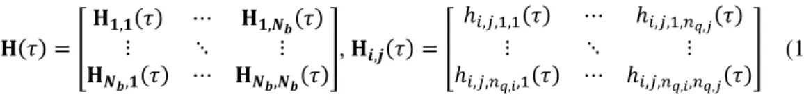
]𝑻 is a vector of average normalized heat extraction rates per unit borehole length along all segments of borehole 𝑗 at time 𝜏𝑝. 𝐇 is a matrix of segment-to-segment thermal
response factors between all pairs of segments in the bore field, given by:
𝐇(𝜏) = [
𝐇
𝟏,𝟏(𝜏)
⋯
𝐇
𝟏,𝑵𝒃(𝜏)
⋮
⋱
⋮
𝐇
𝑵𝒃,𝟏(𝜏) ⋯ 𝐇
𝑵𝒃,𝑵𝒃(𝜏)
], 𝐇
𝒊,𝒋(𝜏) = [
ℎ
𝑖,𝑗,1,1(𝜏)
⋯
ℎ
𝑖,𝑗,1,𝑛𝑞,𝑗(𝜏)
⋮
⋱
⋮
ℎ
𝑖,𝑗,𝑛𝑞,𝑖,1(𝜏) ⋯ ℎ
𝑖,𝑗,𝑛𝑞,𝑖,𝑛𝑞,𝑗(𝜏)
]
(11)
Equation 10 is further simplified by separating the contribution of heat extraction at times preceding time 𝜏𝑘 from the present time 𝜏𝑘:
𝚯
̅
𝒃,𝒌= 𝚯
̅
𝒃,𝒌𝟎+ 𝐇(𝜏
𝑘− 𝜏
𝑘−1)𝚽
̅
𝒌′(12)
𝚯
̅
𝒃,𝒌𝟎= ∑
𝑘−1𝑝=1(𝐇(𝜏
𝑘− 𝜏
𝑝−1) − 𝐇(𝜏
𝑘− 𝜏
𝑝)) 𝚽
̅
𝒑′(13)
Quasi-steady-state heat transfer in the borehole region
Quasi-steady-state heat transfer inside the boreholes can be represented as a circuit of thermal resistances, as shown on Figure 2 for a double (𝑛𝑝,𝑖 = 2) U-tube borehole. Heat transfer between the fluid
flowing inside the pipes and the borehole wall is strictly two-dimensional (over the borehole cross-section); axial heat conduction in the pipes and the grout is neglected. Each borehole 𝑖 has 𝑛𝑝,𝑖 U-tubes (2𝑛𝑝,𝑖 pipes).
Each pipe 𝑚 is connected to pipe 𝑚 + 𝑛𝑝,𝑖 at the bottom of the borehole.
Assuming steady-state heat transfer in the borehole (i.e. the thermal capacities of the fluid, pipes and grout are neglected), the fluid temperature variation along the boreholes are obtained from the following energy balance on the fluid over a borehole cross-section:
𝑚̇
𝑖,𝑚𝑐
𝑓 𝜕𝑇𝑓,𝑖,𝑚 𝜕𝑧(𝑧) =
𝑇𝑓,𝑖,𝑚(𝑧)−𝑇𝑏,𝑖(𝑧) 𝑅𝑖,𝑚,𝑚Δ+ ∑
𝑇𝑓,𝑖,𝑚(𝑧)−𝑇𝑓,𝑖,𝑛(𝑧) 𝑅𝑖,𝑚,𝑛Δ 𝑛𝑝,𝑖 𝑛=1 𝑛≠𝑚, 0 ≤ 𝑧 ≤ 𝐿
𝑖, 𝑚 ≤ 𝑛
𝑝,𝑖(14)
−𝑚̇𝑖,𝑚𝑐𝑓 𝜕𝑇𝑓,𝑖,𝑚 𝜕𝑧 (𝑧) = 𝑇𝑓,𝑖,𝑚(𝑧)−𝑇𝑏,𝑖(𝑧) 𝑅𝑖,𝑚,𝑚Δ + ∑ 𝑇𝑓,𝑖,𝑚(𝑧)−𝑇𝑓,𝑖,𝑛(𝑧) 𝑅𝑖,𝑚,𝑛Δ 𝑛𝑝,𝑖 𝑛=1 𝑛≠𝑚 , 0 ≤ 𝑧 ≤ 𝐿𝑖, 𝑛𝑝,𝑖+ 1 ≤ 𝑚 ≤ 2𝑛𝑝,𝑖(15)
where 𝑚̇𝑖,𝑚 is the fluid mass flow rate in pipes 𝑚 and 𝑚 + 𝑛𝑝,𝑖, and 𝑇𝑓,𝑖,𝑚 is the fluid temperature in
pipe 𝑚 of borehole 𝑖. 𝑅𝑖,𝑚,𝑛Δ is the delta-circuit thermal resistance between pipes 𝑚 and 𝑛 of borehole 𝑖 and
𝑅𝑖,𝑚,𝑚Δ is the delta-circuit thermal resistance between pipe 𝑚 and the wall of borehole 𝑖. These delta-circuit
thermal resistances can be evaluated from the multipole solution (Claesson and Hellström 2011). In this work, the multipole solution of order 3 was used to evaluate delta-circuit thermal resistances.
It is again useful to introduce dimensionless parameters by considering the dimensionless form of Equation 2:
𝜃̅
𝑓(𝜏) =
1 2(𝜃
𝑓,𝑖𝑛(𝜏) + 𝜃
𝑓,𝑜𝑢𝑡(𝜏)) = 𝜃
𝑏 ∗(𝜏) + Ω
𝑓𝑖𝑒𝑙𝑑∗𝜙̅
′(𝜏)
(16)
where 𝜃̅𝑓 is the dimensionless mean fluid temperature, 𝜃𝑓,𝑖𝑛 and 𝜃𝑓,𝑜𝑢𝑡 are the dimensionless inlet and
outlet fluid temperatures of the bore field, Ω𝑓𝑖𝑒𝑙𝑑∗ = 2π𝑘𝑠𝑅𝑓𝑖𝑒𝑙𝑑∗ is the dimensionless effective bore field
thermal resistance.
The dimensionless forms of Equations 14 and 15 are then: 𝜕𝜃𝑓,𝑖,𝑚 𝜕𝜂
(𝜂) =
𝜃𝑓,𝑖,𝑚(𝜂)−𝜃𝑏,𝑖(𝜂) 𝛾𝑖Ω𝑖,𝑚,𝑚Δ+ ∑
𝜃𝑓,𝑖,𝑚(𝜂)−𝜃𝑓,𝑖,𝑛(𝜂) 𝛾𝑖Ω𝑖,𝑚,𝑛Δ 𝑛𝑝,𝑖 𝑛=1 𝑛≠𝑚, 0 ≤ 𝜂 ≤ 1, 𝑚 ≤ 𝑛
𝑝,𝑖(17)
𝜕𝜃𝑓,𝑖,𝑚 𝜕𝜂 (𝜂) = 𝜃𝑓,𝑖,𝑚(𝜂)−𝜃𝑏,𝑖(𝜂) −𝛾𝑖Ω𝑖,𝑚,𝑚Δ + ∑ 𝜃𝑓,𝑖,𝑚(𝜂)−𝜃𝑓,𝑖,𝑛(𝜂) −𝛾𝑖Ω𝑖,𝑚,𝑛Δ 𝑛𝑝,𝑖 𝑛=1 𝑛≠𝑚 , 0 ≤ 𝜂 ≤ 1, 𝑛𝑝,𝑖+ 1 ≤ 𝑚 ≤ 2𝑛𝑝,𝑖(18)
where 𝜃𝑓,𝑖,𝑚 is the dimensionless fluid temperature in pipe 𝑚 of borehole 𝑖, Ω𝑖,𝑚,𝑛Δ and Ω𝑖,𝑚,𝑚Δ are
dimensionless delta-circuit thermal resistances, 𝛾𝑖= 𝑚̇𝑖𝑐𝑓⁄2𝜋𝑘𝑠𝐿𝑖 is the dimensionless fluid mass flow rate
in borehole 𝑖, and 𝜂 is the normalized depth along the length of the borehole. Equations 17 and 18 may then be simplified by introducing matrix notation:
𝜕𝚯𝒇,𝒊
𝜕𝜂
(𝜂) = 𝚪
𝒊(𝚯
𝒇,𝒊(𝜂) − 𝟏𝜃
𝑏,𝑖(𝜂)) , 0 ≤ 𝜂 ≤ 1
(19)
where 𝚯𝒇,𝒊(𝜂) = [𝜃𝑓,𝑖,1 ⋯ 𝜃𝑓,𝑖,2𝑛𝑝,𝑖]
𝑻
is a vector of dimensionless fluid temperatures in each pipe of borehole 𝑖, 𝚪𝒊= [𝛤𝑖,𝑚,𝑛]2𝑛
𝑝,𝑖×2𝑛𝑝,𝑖 is a dimensionless thermal conductance matrix, given by:
𝛤
𝑖,𝑚,𝑛=
{
∑
(𝛾
𝑖Ω
𝑖,𝑚,𝑛Δ)
−1 𝑚 𝑛=1for 𝑚 = 𝑛 and 𝑚 ≤ 𝑛
𝑝,𝑖−(𝛾
𝑖Ω
𝑖,𝑚,𝑛Δ)
−1for 𝑚 ≠ 𝑛 and 𝑚 ≤ 𝑛
𝑝,𝑖− ∑
(𝛾
𝑖Ω
𝑖,𝑚,𝑛Δ)
−1 𝑚 𝑛=1for 𝑚 = 𝑛 and 𝑛
𝑝,𝑖+ 1 ≤ 𝑚 ≤ 2𝑛
𝑝,𝑖(𝛾
𝑖Ω
𝑖,𝑚,𝑛Δ)
−1for 𝑚 ≠ 𝑛 and 𝑛
𝑝,𝑖+ 1 ≤ 𝑚 ≤ 2𝑛
𝑝,𝑖(20)
The solution to Equation 19 is given by the matrix exponential (Cimmino 2016):
𝚯
𝒇,𝒊(𝜂) = exp(𝚪
𝒊𝜂) 𝚯
𝒇,𝒊(0) − ∫ exp(𝚪
𝒊(𝜂 − 𝜂
′)) 𝚪
𝒊𝟏𝜃
𝑏,𝑖(𝜂
′)𝑑𝜂
′ 𝜂0
(21)
This solution gives the fluid temperature variation along the borehole for an arbitrary borehole wall temperature. From this solution, it is possible, considering piping connections within the borehole (series or parallel), to obtain linear relations between the inlet and outlet fluid temperatures of the borehole and between the inlet fluid temperature into the borehole and the heat extraction rate per unit length along the borehole. For a borehole 𝑖 divided into 𝑛𝑞,𝑖 segments of equal lengths with uniform temperature along the wall of each
segment, these relations are given by:
𝜃
𝑓,out,𝑖,𝑘= E
in,𝑖 𝜃𝑜𝑢𝑡𝜃
𝑓,in,𝑖,𝑘+ 𝐄
𝒃,𝒊 𝜽𝒐𝒖𝒕𝚯
̅
𝒃,𝒊,𝒌(22)
𝚽
̅
𝒊,𝒌′= 𝐄
𝐢𝐧,𝒊 𝝓𝜃
𝑓,in,𝑖,𝑘+ 𝐄
𝒃,𝒊 𝝓𝚯
̅
𝒃,𝒊,𝒌(23)
where 𝜃𝑓,in,𝑖,𝑘 and 𝜃𝑓,out,𝑖,𝑘 are the dimensionless inlet and outlet fluid temperatures of borehole 𝑖 at time
𝜏𝑘, and Ein,𝑖 𝜃𝑜𝑢𝑡 , 𝐄𝒃,𝒊 𝜽𝒐𝒖𝒕 , 𝐄𝐢𝐧,𝒊 𝝓 and 𝐄 𝒃,𝒊
𝝓 are coefficients with values developed in appendices 1 and 2.
Piping connections in the network of boreholes
In bore fields with mixed parallel and series connections between the boreholes, the inlet fluid temperature into a borehole 𝑖 may be different from the inlet fluid temperature into the bore field and is determined by the arrangement of the borehole network. The inlet fluid temperature into borehole 𝑖 is either
equal to the inlet fluid temperature into the field or to the outlet fluid temperature of another borehole. The arrangement of the borehole network is represented by a borehole connectivity vector:
𝜃
𝑓,in,𝑖,𝑘= 𝜃
𝑓,out,𝑐in,𝑖,𝑘(24)
where 𝐂𝐢𝐧= [𝑐in,1 ⋯ 𝑐in,𝑁𝑏] is the borehole connectivity vector, with 𝑐in,𝑖 the index of the borehole
connected to the inlet of borehole 𝑖 (e.g. 𝑐in,2= 1 in Figure 1); and 𝜃𝑓,out,0,𝑘 = 𝜃𝑓,in,𝑘 is the inlet fluid
temperature into the bore field (e.g. 𝑐in,1= 0 in Figure 1). For example, for the bore field represented in
Figure 1, the borehole connectivity vector is 𝐂𝐢𝐧= [0 1 0]. For convenience, the sequence 𝐏𝐢𝐧,𝐢 denotes
the path starting from borehole 𝑖 leading to the bore field inlet. With regards to the bore field of Figure 1: 𝐏𝐢𝐧,𝟏 = {1}, 𝐏𝐢𝐧,𝟐= {2,1} and 𝐏𝐢𝐧,𝟑= {3}.
From Equation 22 and with knowledge of the borehole connectivity, the outlet fluid temperature at any borehole can be expressed in terms of the inlet fluid temperature of the field and the borehole wall temperatures of all boreholes in its path to the inlet:
𝜃
𝑓,out,𝑖,𝑘= (∏
E
in,𝑖 𝜃𝑜𝑢𝑡 𝑗∈𝐏𝐢𝐧,𝒊) 𝜃
𝑓,in,𝑘+ ∑
(∏
E
in,𝑗′ 𝜃𝑜𝑢𝑡 𝑗′∈𝐏 𝐢𝐧,𝒊 𝑗′∉𝐏 𝐢𝐧,𝒋) 𝐄
𝒃,𝒋𝜽𝒐𝒖𝒕𝚯
̅
𝒃,𝒋,𝒌 𝑗∈𝐏𝐢𝐧,𝒊(25)
𝜃
𝑓,out,𝑖,𝑘= A
in,𝑖 𝜃𝑜𝑢𝑡𝜃
𝑓,in,𝑘+ ∑
𝐀
𝒃,𝒊,𝒋 𝜽𝒐𝒖𝒕𝚯
̅
𝒃,𝒋,𝒌 𝑗∈𝐏𝐢𝐧,𝒊(26)
where Ain,𝑖 𝜃𝑜𝑢𝑡 and 𝐀 𝒃,𝒊,𝒋𝜽𝒐𝒖𝒕 are scalar and vector coefficients, with 𝐀
𝒃,𝒊,𝒋
𝜽𝒐𝒖𝒕= 𝟎 if 𝑗 ∉ 𝐏
𝐢𝐧,𝒊, Π is the product
operator, with ∏ Ein,𝑖𝜃𝑜𝑢𝑡
𝑗∈{1,2,3} = Ein,1 𝜃𝑜𝑢𝑡E in,2 𝜃𝑜𝑢𝑡E in,3 𝜃𝑜𝑢𝑡 and ∏ E in,𝑖 𝜃 𝑗∈{ } = 1.
From Equations 23 and 25, and considering the borehole connectivity, the heat extraction rate per unit borehole length of any borehole may also be expressed in terms of the inlet fluid temperature of the field and the borehole wall temperatures of all boreholes in its path to the inlet:
𝚽
̅
𝒊,𝒌′= 𝐄
𝐢𝐧,𝒊𝝓(∏
E
in,𝑗𝜃𝑜𝑢𝑡 𝑗∈𝐏𝐢𝐧,𝒊 𝑗≠𝑖) 𝜃
𝑓,in,𝑘+ ∑
(∏
E
in,𝑗′ 𝜃𝑜𝑢𝑡 𝑗′∈𝐏 𝐢𝐧,𝒊 𝑗′∉𝐏 𝐢𝐧,𝒋) 𝐄
𝒃,𝒋𝝓𝚯
̅
𝒃,𝒋,𝒌 𝑗∈𝐏𝐢𝐧,𝒊(27)
𝚽
̅
𝒊,𝒌′= 𝐀
𝝓𝐢𝐧,𝒊𝜃
𝑓,in,𝑘+ ∑
𝐀
𝒃,𝒊,𝒋 𝝓𝚯
̅
𝒃,𝒋,𝒌 𝑗∈𝐏𝐢𝐧,𝒊(28)
where 𝐀𝐢𝐧,𝒊 𝝓 and 𝐀 𝒃,𝒊,𝒋𝝓 are vector and matrix coefficients, with 𝐀 𝒃,𝒊,𝒋
𝝓 = 𝟎 if 𝑗 ∉ 𝐏 𝐢𝐧,𝒊.
The heat extraction rates per unit borehole length of all borehole segments are then given by assembling Equation 28 for all boreholes in the field:
𝚽
̅
𝒌′= 𝐀
𝐢𝐧 𝝓𝜃
𝑓,in,𝑘+ 𝐀
𝒃 𝝓𝚯
̅
𝒃,𝒌(29)
𝐀
𝝓𝐢𝐧= [
𝐀
𝝓𝐢𝐧,𝟏⋮
𝐀
𝐢𝐧,𝑵 𝒃 𝝓]
(30)
𝐀
𝝓𝐛= [
𝐀
𝝓𝒃,𝟏,𝟏⋯
𝐀
𝒃,𝟏,𝑵 𝒃 𝝓⋮
⋱
⋮
𝐀
𝒃,𝑵 𝒃,𝟏 𝝓⋯ 𝐀
𝒃,𝑵 𝒃,𝑵𝒃 𝝓]
(31)
The outlet fluid temperature of the bore field is obtained by an energy balance:
𝜃
𝑓,out,𝑘= 𝜃
𝑓,in,𝑘− 𝑁
𝑏 𝜙̅𝑘′ 𝛾(32)
𝜃
𝑓,out,𝑘= (1 −
1 𝛾 𝐋 𝐿̅𝐀
𝐢𝐧 𝝓) 𝜃
𝑓,in,𝑘−
1 𝛾 𝐋 𝐿̅𝐀
𝒃 𝝓𝚯
̅
𝒃,𝒌(33)
𝜃
𝑓,out,𝑘= A
in 𝜃𝑜𝑢𝑡𝜃
𝑓,in,𝑘+ 𝐀
𝒃 𝜽𝒐𝒖𝒕𝚯
̅
𝒃,𝒌(34)
where 𝛾 = 𝑚̇𝑐𝑓⁄2𝜋𝑘𝑠𝐿̅ is the dimensionless total fluid mass flow rate, 𝜙̅𝑘′ = 𝐋𝚽̅𝒌′⁄𝑁𝑏𝐿̅ is the
normalized average heat extraction rate per unit borehole length in the bore field, 𝐋 = [𝐋𝟏 ⋯ 𝐋𝑵𝒃] is a
vector of the lengths of all borehole segments in the bore field, with 𝐋𝐢 = [𝐿𝑖,1 ⋯ 𝐿𝑖,𝑛𝑞,𝑖].
g-Function of the bore field
Dimensionless borehole wall and inlet fluid temperatures
Per the definition of the g-function (Equations 1 and 8), the g-function is obtained from the dimensionless borehole wall temperature response to a constant unit normalized heat extraction rate per borehole length:
𝜙̅
𝑘′= 𝐋𝚽
̅
𝒌′⁄
𝑁
𝑏𝐿̅
= 1
(35)
The dimensionless borehole wall and inlet fluid temperature responses are obtained by the simultaneous solution of Equations 12, 29 and 35:
[
𝐇(𝜏
𝑘− 𝜏
𝑘−1)
−𝐈
𝟎
−𝐈
𝐀
𝝓𝒃𝐀
𝝓𝐢𝐧𝐋 𝑁
⁄
𝑏𝐿̅
𝟎
0
] [
𝚽
̅
𝒌′𝚯
̅
𝒃,𝒌𝜃
𝑓,in,𝑘] = [
−𝚯
̅
𝒃,𝒌𝟎𝟎
1
]
(36)
where 𝐈 is the identity matrix.
Effective borehole and bore field thermal resistances
To evaluate the effective dimensionless borehole wall temperature – and thus the g-function – the effective bore field thermal resistance (defined by Equations 2 and 16) must first be evaluated. The concept of effective borehole thermal resistance was first introduced by Hellström (1991), who considered a uniform borehole wall temperature and obtained the effective borehole thermal resistance based on the arithmetic mean fluid temperature:
Ω
𝑏,𝑖∗=
1
2(𝜃𝑓,in,𝑖,𝑘+𝜃𝑓,out,𝑖,𝑘)−𝜃𝑏,𝑖,𝑘 ∗
𝜙̅𝑖,𝑘′
(37)
where 𝜙̅𝑖,𝑘′ = 𝐋𝒊𝚽̅𝒊,𝒌′ ⁄𝐿𝑖 is the average normalized heat extraction rate per unit length of borehole 𝑖, 𝜃𝑏,𝑖,𝑘∗
is the effective uniform dimensionless borehole wall temperature of borehole 𝑖, and Ω𝑏,𝑖∗ = 2𝜋𝑘𝑠𝑅𝑏,𝑖∗ is the
effective dimensionless borehole thermal resistance of borehole 𝑖.
From Equations 22 and 23 and assuming a zero dimensionless borehole wall temperature, 𝜃𝑏,𝑖,𝑘∗ = 0:
Ω
𝑏,𝑖∗=
1 2∙
1+Ein,𝑖𝜃𝑜𝑢𝑡
𝐋𝒊𝐄𝐢𝐧,𝒊𝝓 ⁄𝐿𝑖
(38)
Similarly, the bore field thermal resistance is defined as the ratio of the temperature difference between the arithmetic mean fluid temperature in the bore field and the effective borehole wall temperature, and the average heat extraction rate per unit borehole length in the bore field, considering a uniform effective borehole wall temperature across the bore field:
Ω
𝑓𝑖𝑒𝑙𝑑∗=
1 2(𝜃𝑓,in,𝑘+𝜃𝑓,out,𝑘)−𝜃𝑏,𝑘 ∗ 𝜙̅ 𝑘 ′(39)
From Equations 29 and 34 and assuming a zero dimensionless borehole wall temperature, 𝜃𝑏,𝑖,𝑘∗ = 0:
Ω
𝑓𝑖𝑒𝑙𝑑∗=
1 2∙
1+Ain𝜃𝑜𝑢𝑡
Effective dimensionless borehole wall temperature
The solution of Equation 36 gives the variation of the dimensionless inlet fluid temperature into the bore field. From Equations 16 and 32, the effective dimensionless borehole wall temperature is given by:
𝜃
𝑏∗(𝜏
𝑘) = 𝜃
𝑓,in,𝑘−
𝑁𝑏2𝛾
− Ω
𝑓𝑖𝑒𝑙𝑑∗
(41)
where 𝜃𝑏∗ is the effective dimensionless borehole wall temperature, equal to the g-function of the bore
field. In combination with the effective bore field thermal resistance, the g-function permits the simulation of fluid temperatures in geothermal bore fields with series- and parallel-connected boreholes. An example of the complete calculation process for the evaluation of the g-function of a field of 2 series-connected boreholes is detailed in Appendix 3.
Results
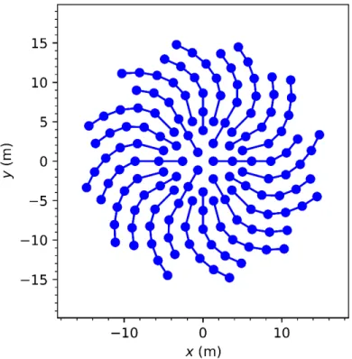
A field of 144 boreholes is shown on Figure 3. The field consists of 24 parallel branches of 6 series-connected single U-tube boreholes of equal dimensions. The dimensional and physical parameters of the bore field are presented in Table 1. Fluid enters the 24 parallel branches from the center of the field and exits from its perimeter. The fluid mass flow rate is evenly distributed across all branches. The effective borehole thermal resistance is 𝑅𝑏∗ = 0.1460 m-K/W, corresponding to a dimensionless effective borehole thermal
resistance of Ω𝑏∗ = 1.835. The effective bore field thermal resistance is 𝑅𝑓𝑖𝑒𝑙𝑑∗ = 0.1700 m-K/W,
corresponding to a dimensionless effective borehole thermal resistance of Ω𝑓𝑖𝑒𝑙𝑑∗ = 2.136. The dimensionless
total fluid mass flow rate is 𝛾 = 54.25. With regards to the number of boreholes, the number of parallel branches, the length of the boreholes and the average spacing between the boreholes, the bore field in Figure 3 is similar to the borehole thermal energy storage of Drake Landing Solar Community (Sibbitt et al. 2012). In this section, the presented g-function calculation method is compared to the results of simulations obtained using the duct ground heat storage (DST) model (Pahud and Hellström 1996). The effect of fluid mass flow rate on the g-function and on the effective bore field thermal resistance is then studied.
Figure 3. Bore field of 144 boreholes in 24 parallel branches of 6 series-connected boreholes Table 1. Parameters of the bore field
Parameter Value Units
Bore field
Number of boreholes, 𝑁𝑏 144 -
Number of parallel branches 24 -
Boreholes per branch 6 -
Nominal borehole spacing 2.25 m
Total fluid mass flow rate, 𝑚̇ 6 kg/s
Boreholes
Borehole length, 𝐿 35 m
Borehole radius, 𝑟𝑏 0.075 m
Borehole buried depth, 𝐷 0.5 m
Piping
Number of U-tubes per borehole, 𝑛𝑝 1 -
Pipe outer diameter 0.0422 m
Pipe inner diameter 0.0294 m
Shank spacing 0.052 m
Pipe surface roughness 10-6 m
Physical properties
Undisturbed ground temperature, 𝑇0 10 °C
Ground thermal conductivity, 𝑘𝑠 2 W/m-K
Ground thermal diffusivity, 𝛼𝑠 10-6 m2/s
Grout thermal conductivity 1 W/m-K
Pipe thermal conductivity 0.4 W/m-K
Fluid thermal conductivity 0.492 W/m-K
Fluid density 1015 kg/m3
Fluid specific heat capacity, 𝑐𝑓 3977 J/kg-K
g-Function of the bore field
The effective dimensionless borehole wall temperature (i.e. the g-function) and the dimensionless inlet fluid temperature obtained from the presented methodology are shown on Figure 4, using 𝑛𝑞 = 12 segments
per borehole. The dimensionless temperatures are compared to the average storage temperature and the inlet fluid temperature obtained from a constant heat injection simulation using the DST model. As the DST model does not consider the positions of the boreholes in the bore field, but rather assumes evenly distributed boreholes in a specified storage volume, a storage volume of 25,270 m3 given by the cylindrical volume
delimited by the boreholes furthest from the center of the field was used for this simulation. The simulation was performed with a time step of 1 hour over a simulation period of 100 years and a constant heat injection rate 𝑄̅′= 2𝜋𝑘
𝑆. The effective borehole wall temperature is not directly comparable to the average storage
temperature, as the former is representative of the temperature in the immediate vicinity of the boreholes while the latter is representative of the average temperature in the volume. For this reason, the inlet fluid temperatures are better suited for comparison between the g-function and the DST model (Pahud and Hellström 1996). The results are close, with a maximum absolute difference of 1.46 at ln(𝜏) = 1.8 when the dimensionless inlet fluid temperature is 54.02, and a maximum relative difference of 4.2 % at ln(𝜏) = -9.9 corresponding to the second time step of the DST simulation. Differences are expected since the DST model does not consider the actual positions of the boreholes.
The calculation time for the evaluation of the g-function of the field of 144 boreholes over 100 time steps using 𝑛𝑞 = 12 segments per borehole is 447 seconds on a computer equipped with a 4.2 GHz quad core
(8 threads) processor. Comparatively, the calculation time for the evaluation of the g-function of the same
bore field using a uniform borehole wall temperature condition as per the method of Cimmino and Bernier (2014) and Cimmino (2018c) (i.e. without consideration for the fluid temperature variations and the connections between boreholes) is 412 seconds. The time difference is caused by the increased size of the system of equations solved in Equation 36, as the time required for the evaluation of the matrix of segment-to-segment thermal response factors, 𝐇, is 220 seconds in both cases.
Figure 4. Comparison of the dimensionless effective borehole wall and inlet fluid temperatures with the DST model
Simulation of a seasonal storage system
The g-function of the bore field presented in Figure 4 is used in a sample simulation of a seasonal thermal energy storage system. Simplified relations are used for the total heat extraction from the bore field, given as the sum of heat extraction due to building heating loads and solar thermal collectors (heat injection corresponds to negative heat extraction). The building heating loads, 𝑄𝑏𝑢𝑖𝑙𝑑𝑖𝑛𝑔𝑠, are represented by a linear
relation with ambient temperature:
𝑄
𝑏𝑢𝑖𝑙𝑑𝑖𝑛𝑔𝑠= max(0, −7500[𝑊 𝐾
⁄ ] ∙ 𝑇
𝑎𝑚𝑏+ 75000[𝑊])
(42)
where 𝑇𝑎𝑚𝑏 is the ambient temperature (in °C), averaged over the 6 preceding hours, obtained from asolar heat injection started at the beginning of the system’s operation, on January 1st, while building heating
loads were only applied at the beginning of the following heating season, in September of the first year. The heat extraction rate from solar collectors is given by:
𝑄
𝑠𝑜𝑙𝑎𝑟= −𝐴
𝑐𝑜𝑙𝜂𝐺
(43)
where 𝐴𝑐𝑜𝑙= 750 m2 is the total solar collector area, 𝜂 = 0.6 is a constant solar collector efficiency and
𝐺 is the total solar radiation on solar collectors facing due south with a slope of 45°, obtained for the same typical meteorological year.
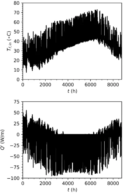
A 5 year simulation of the seasonal thermal storage system was conducted with the DST model with a time step of 1 hour. Using the same ground heat extraction rates, the effective borehole wall temperature were obtained from the temporal superposition of the g-function, using the FFT technique proposed by Marcotte and Pasquier (2008). The inlet fluid temperatures were then obtained from Equation 2. The inlet fluid temperatures during the 5th simulation year predicted from the temporal superposition of the g-function
are presented on Figure 5, along with the average heat extraction rate per unit borehole length. Predicted inlet fluid temperatures are in good agreement with the DST model, as shown on Figure 6 for a 5 day period of the 5th simulation year, starting on June 30th. This 5 day period coincides with the maximum difference of
Figure 5. Inlet fluid temperature during the 5th simulation year (above), and average heat extraction rate per unit borehole length (below)
Figure 6. Comparison of the inlet fluid temperatures predicted by the g-function and the DST model (above), difference between the two models (center), and average heat extraction rate per unit
borehole length (below)
Fluid mass flow rate
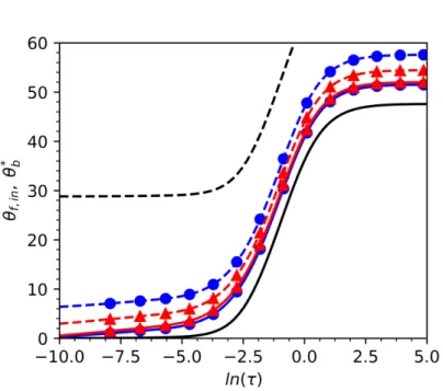
The influence of the fluid mass flow rate on the g-function is presented on Figure 7. It is shown that the difference between the inlet fluid temperature and the effective borehole wall temperature increases when the mass flow rate is reduced, as predicted by Equation 41. It is also shown that, for sufficiently large mass flow rates, the effective dimensionless borehole wall temperature does not show significant variations. At
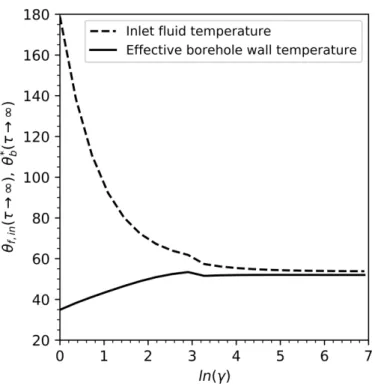
ln(𝜏) = 5, the values of the effective dimensionless borehole wall temperature are 51.5 and 52.0 for dimensionless fluid mass flow rates of 𝛾 = 25 and 125, respectively. These results imply that, for sufficiently large mass flow rates, the same g-function can be used for simulation. The effect of the fluid mass flow rate is further demonstrated on Figure 8, comparing the steady-state dimensionless inlet fluid temperature and effective dimensionless borehole wall temperature at varying mass flow rates. For the bore field of Figure 3, the steady-state effective borehole wall temperature only varies by 1 % for 𝛾 ≥ 21.8. The sharp variation around ln(𝜏) = 3 is due to the transition from laminar to turbulent flow within the boreholes. The variations of the effective dimensionless borehole wall temperature are explained by the variations of the effective bore field thermal resistance, as shown on Figure 9. In the same range 𝛾 ≥ 21.8, the effective bore field thermal resistance varies from 4.07 to 1.76. These results are in agreement to that of Cimmino (2015) who found that, for parallel-connected boreholes, the values of the g-function depend on the effective borehole thermal resistance. It should be noted that, for infinite mass flow rate (i.e. 𝛾 → ∞), the effective bore field thermal resistance (defined in Equation 2) tends to the same value as the effective borehole thermal resistance.
Figure 7. Influence of the dimensionless fluid mass flow rate on the dimensionless inlet fluid temperature and on the effective dimensionless borehole wall temperature
Figure 8. Influence of the dimensionless fluid mass flow rate on the steady-state dimensionless effective borehole wall temperature and on the steady-state dimensionless inlet fluid temperature
Figure 9. Influence of the dimensionless fluid mass flow rate on the effective borehole thermal resistance and the effective bore field thermal resistance
Conclusion
A semi-analytical method for the calculation of g-functions of bore fields with mixed arrangements of series- and parallel-connected boreholes is presented. Borehole wall temperature variations are obtained from the temporal and spatial superposition of the finite line source solution. Heat transfer between the fluid and the borehole wall is obtained from an analytical solution based on an energy balance on a thermal resistance network representing a borehole cross-section. The concept of effective bore field thermal resistances is introduced and is used in the definition of the effective borehole wall temperature. This yields a linear relation between the arithmetic mean fluid temperature, the heat extraction rate per unit borehole length and the effective bore field thermal resistance, as is typically encountered in simulations of parallel-connected borehole fields.
The g-function calculation method is validated against the DST model on a bore field consisting of 24 parallel branches of 6 series-connected boreholes, totalling 144 boreholes. Some small differences in predicted inlet fluid temperatures are observed but can be explained by the fundamental differences between the two methods, i.e. the positions of the boreholes are not explicitly prescribed in the DST model. The g-function is shown to be dependent on the fluid mass flow rate, although variations in g-function values are not significant at sufficiently high fluid mass flow rates. An important limitation of the proposed method is that it is not possible to account for changes in flow direction within the bore field, which can be expected in seasonal storage systems. This limitation will be addressed in future work.
Nomenclature
A, 𝐀 : Coefficient, vector of coefficients or matrix of coefficients 𝐂𝐢𝐧 : Borehole connectivity vector
𝑐𝑓 : Fluid specific heat capacity, J/kg-K
𝐷 : Buried depth, m 𝑑 : Distance, m
E, 𝐄 : Coefficient, vector of coefficients or matrix of coefficients 𝐺 : Total incident solar radiation
𝑔 : g-function
𝐇 : Matrix of segment-to-segment thermal response factors ℎ : Segment-to-segment thermal response factor
𝐼𝐹𝐿𝑆 : Axial portion of the integrand function of the finite line source solution
𝑘 : Thermal conductivity, W/m-K 𝐿 : Length, m
𝑚̇ : Mass flow rate, kg/s 𝑁𝑏 : Number of boreholes
𝑛𝑝 : Number of U-tubes
𝑛𝑞 : Number of borehole segments
𝐏𝐢𝐧 : Path sequence to bore field inlet
𝑄 : Heat extraction rate, W
𝑄′ : Heat extraction rate per unit length, W/m
𝑅 : Thermal resistance, m-K/W 𝑟 : Radius, m
𝑇 : Temperature, ºC 𝑡 : Time, s
(𝑥, 𝑦) : Borehole horizontal coordinates, m 𝐘 : Vector of dimensionless fluid mass flow rates 𝑧 : Vertical coordinate, m
Greek symbols
𝛼 : Thermal diffusivity, m2/s
𝚪 : Dimensionless thermal conductance matrix 𝛾 : Dimensionless fluid mass flow rate 𝜂 : Dimensionless vertical coordinate 𝚯 : Vector of dimensionless temperatures 𝜃 : Dimensionless temperature
𝜌 : Density, kg/m3
𝜏 : Dimensionless time
𝚽′ : Vector of dimensionless heat extraction rates per unit length
𝜙′ : Dimensionless heat extraction rate per unit length
Ω : Dimensionless thermal resistance
Subscripts
0 : Initial
𝑏 : Borehole, or borehole wall (temperature) 𝑓 : Fluid
𝑓𝑖𝑒𝑙𝑑 : Bore field 𝑖, 𝑗 : Borehole indices 𝑖𝑛 : Inlet
𝑘, 𝑝 : Time step indices 𝑚, 𝑛 : Pipe indices 𝑛𝑜𝑚 : Nominal value 𝑜𝑢𝑡 : Outlet
𝑠 : Soil
𝑠𝑡𝑜𝑟𝑎𝑔𝑒 : Storage (DST model) 𝑢, 𝑣 : Borehole segment indices
Superscripts
( )∗ : Effective value
( )Δ : Delta-circuit
References
Abdelaziz, S. L., T. Y. Ozudogru, C. G. Olgun, and J. R. Martin. 2014. “Multilayer Finite Line Source Model for Vertical Heat Exchangers.” Geothermics 51: 406–416.
doi:10.1016/j.geothermics.2014.03.004.
ASHRAE. 2015. ASHRAE Handbook — HVAC Applications. Atlanta GA, USA: American Society of Heating, Refrigerating and Air Conditioning Engineers.
Bandyopadhyay, G., W. Gosnold, and M. Mann. 2008. “Analytical and Semi-Analytical Solutions for Short-Time Transient Response of Ground Heat Exchangers.” Energy and Buildings 40 (10). Elsevier: 1816–1824. doi:10.1016/J.ENBUILD.2008.04.005.
Beier, R. A., and M. D. Smith. 2003. “Minimum Duration of In-Situ Tests on Vertical Boreholes.” ASHRAE Transactions 109: 475–486.
Cimmino, M. 2015. “The Effects of Borehole Thermal Resistances and Fluid Flow Rate on the G-Functions of Geothermal Bore Fields.” International Journal of Heat and Mass Transfer 91: 1119– 1127. doi:10.1016/j.ijheatmasstransfer.2015.08.041.
Cimmino, M. 2016. “Fluid and Borehole Wall Temperature Profiles in Vertical Geothermal Boreholes with Multiple U-Tubes.” Renewable Energy 96: 137–147. doi:10.1016/j.renene.2016.04.067.
Cimmino, M. 2018a. “A Finite Line Source Simulation Model for Geothermal Systems with Series- and Parallel-Connected Boreholes and Independent Fluid Loops.” Journal of Building Performance Simulation 11 (4): 414–432. doi:10.1080/19401493.2017.1381993.
Cimmino, M. 2018b. “G-Functions for Bore Fields with Mixed Parallel and Series Connections
Considering Axial Fluid Temperature Variations.” In Proceedings of the IGSHPA Research Track 2018, 262–270. International Ground Source Heat Pump Association.
doi:10.22488/okstate.18.000015.
Cimmino, M. 2018c. “Fast Calculation of the G-Functions of Geothermal Borehole Fields Using
Similarities in the Evaluation of the Finite Line Source Solution.” Journal of Building Performance Simulation 11 (6): 655–668. doi:10.1080/19401493.2017.1423390.
Cimmino, M., and M. Bernier. 2014. “A Semi-Analytical Method to Generate g-Functions for Geothermal Bore Fields.” International Journal of Heat and Mass Transfer 70 (c): 641–650.
doi:10.1016/j.ijheatmasstransfer.2013.11.037.
Cimmino, M., M. Bernier, and F. Adams. 2013. “A Contribution towards the Determination of G-Functions Using the Finite Line Source.” Applied Thermal Engineering 51 (1–2): 401–412.
doi:10.1016/j.applthermaleng.2012.07.044.
Claesson, J., and G. Hellström. 2011. “Multipole Method to Calculate Borehole Thermal Resistances in a Borehole Heat Exchanger.” HVAC&R Research 17 (6): 895–911.
doi:10.1080/10789669.2011.609927.
Claesson, J., and S. Javed. 2011. “An Analytical Method to Calculate Borehole Fluid Temperatures for Time-Scales from Minutes to Decades.” ASHRAE Transactions 117 (2): 279–288.
Cui, P., H. Yang, and Z. Fang. 2006. “Heat Transfer Analysis of Ground Heat Exchangers with Inclined Boreholes.” Applied Thermal Engineering 26 (11–12): 1169–1175.
doi:10.1016/j.applthermaleng.2005.10.034.
Dusseault, B., P. Pasquier, and D. Marcotte. 2018. “A Block Matrix Formulation for Efficient G-Function Construction.” Renewable Energy 121 (June). Pergamon: 249–260.
doi:10.1016/J.RENENE.2017.12.092.
Erol, S., and B. François. 2018. “Multilayer Analytical Model for Vertical Ground Heat Exchanger with Groundwater Flow.” Geothermics 71 (January). Pergamon: 294–305.
Eskilson, P. 1987. “Thermal Analysis of Heat Extraction Boreholes.” University of Lund.
Fossa, M. 2011. “The Temperature Penalty Approach to the Design of Borehole Heat Exchangers for Heat Pump Applications.” Energy and Buildings 43 (6): 1473–1479. doi:10.1016/j.enbuild.2011.02.020. Hellström, G. 1991. “Ground Heat Storage: Thermal Analysis of Duct Storage Systems.” University of
Lund.
Hu, J. 2017. “An Improved Analytical Model for Vertical Borehole Ground Heat Exchanger with Multiple-Layer Substrates and Groundwater Flow.” Applied Energy 202 (September): 537–549.
doi:10.1016/j.apenergy.2017.05.152.
Javed, S., and J. Claesson. 2011. “New Analytical and Numerical Solutions for the Short-Term Analysis of Vertical Ground Heat Exchangers.” ASHRAE Transactions 117: 279–288.
Lamarche, L. 2011. “Analytical G-Function for Inclined Boreholes in Ground-Source Heat Pump Systems.” Geothermics 40 (4): 241–249. doi:10.1016/j.geothermics.2011.07.006.
Lamarche, L., and B. Beauchamp. 2007a. “A New Contribution to the Finite Line-Source Model for Geothermal Boreholes.” Energy and Buildings 39 (2): 188–198. doi:10.1016/j.enbuild.2006.06.003. Lamarche, L., and B. Beauchamp. 2007b. “New Solutions for the Short-Time Analysis of Geothermal
Vertical Boreholes.” International Journal of Heat and Mass Transfer 50 (7–8). Pergamon: 1408– 1419. doi:10.1016/J.IJHEATMASSTRANSFER.2006.09.007.
Lamarche, L. 2015. “Short-Time Analysis of Vertical Boreholes, New Analytic Solutions and Choice of Equivalent Radius.” International Journal of Heat and Mass Transfer 91 (December): 800–807. doi:10.1016/j.ijheatmasstransfer.2015.07.135.
Lamarche, L. 2017a. “Mixed Arrangement of Multiple Input-Output Borehole Systems.” Applied Thermal Engineering. doi:10.1016/j.applthermaleng.2017.06.060.
Lamarche, L. 2017b. “G-Function Generation Using a Piecewise-Linear Profile Applied to Ground Heat Exchangers.” International Journal of Heat and Mass Transfer 115 (December): 354–360. doi:10.1016/j.ijheatmasstransfer.2017.08.051.
Lazzarotto, A. 2014. “A Network-Based Methodology for the Simulation of Borehole Heat Storage Systems.” Renewable Energy 62: 265–275. doi:10.1016/j.renene.2013.07.020.
Lazzarotto, A. 2016. “A Methodology for the Calculation of Response Functions for Geothermal Fields with Arbitrarily Oriented Boreholes – Part 1.” Renewable Energy 86: 1380–1393.
doi:10.1016/j.renene.2015.09.056.
Li, M., and A. C. K. Lai. 2012a. “New Temperature Response Functions (G Functions) for Pile and Borehole Ground Heat Exchangers Based on Composite-Medium Line-Source Theory.” Energy 38 (1). Pergamon: 255–263. doi:10.1016/J.ENERGY.2011.12.004.
Li, M., and A. C. K. Lai. 2012b. “Heat-Source Solutions to Heat Conduction in Anisotropic Media with Application to Pile and Borehole Ground Heat Exchangers.” Applied Energy 96 (August): 451–458. doi:10.1016/j.apenergy.2012.02.084.
Li, M., and A. C. K. Lai. 2013. “Analytical Model for Short-Time Responses of Ground Heat Exchangers with U-Shaped Tubes: Model Development and Validation.” Applied Energy 104 (April). Elsevier: 510–516. doi:10.1016/J.APENERGY.2012.10.057.
Marcotte, D., and P. Pasquier. 2008. “Fast Fluid and Ground Temperature Computation for Geothermal Ground-Loop Heat Exchanger Systems.” Geothermics 37 (6): 651–665.
doi:10.1016/j.geothermics.2008.08.003.
Marcotte, D., and P. Pasquier. 2009. “The Effect of Borehole Inclination on Fluid and Ground Temperature for GLHE Systems.” Geothermics 38 (4): 392–398. doi:10.1016/j.geothermics.2009.06.001.
Marcotte, D., and P. Pasquier. 2014. “Unit-Response Function for Ground Heat Exchanger with Parallel, Series or Mixed Borehole Arrangement.” Renewable Energy 68: 14–24.
doi:10.1016/j.renene.2014.01.023.
Molina-Giraldo, N., P. Blum, K. Zhu, P. Bayer, and Z. Fang. 2011. “A Moving Finite Line Source Model to Simulate Borehole Heat Exchangers with Groundwater Advection.” International Journal of Thermal Sciences 50 (12): 2506–2513. doi:10.1016/j.ijthermalsci.2011.06.012.
Monzó, P., P. Mogensen, J. Acuña, F. Ruiz-Calvo, and C. Montagud. 2015. “A Novel Numerical Approach for Imposing a Temperature Boundary Condition at the Borehole Wall in Borehole Fields.”
Geothermics 56 (July). Pergamon: 35–44. doi:10.1016/J.GEOTHERMICS.2015.03.003.
2018. “Numerical Modeling of Ground Thermal Response with Borehole Heat Exchangers Connected in Parallel.” Energy and Buildings 172 (August). Elsevier: 371–384.
doi:10.1016/J.ENBUILD.2018.04.057.
Naldi, C., and E. Zanchini. 2019. “A New Numerical Method to Determine Isothermal G-Functions of Borehole Heat Exchanger Fields.” Geothermics 77 (January). Pergamon: 278–287.
doi:10.1016/J.GEOTHERMICS.2018.10.007.
Numerical Logics. 1999. “Canadian Weather for Energy Calculations, Users Manual and CD-ROM.” Downsview ON, Canada: Environment Canada.
Pahud, D., and G. Hellström. 1996. “The New Duct Ground Heat Model for TRNSYS.” In Proceedings of Eurotherm Seminar N° 49, edited by A. A. van Steenhoven and W. G. J. van Helden, 127–136. Eindhoven, The Netherlands.
Sibbitt, B., D. McClenahan, R. Djebbar, J. Thornton, B. Wong, J. Carriere, and J. Kokko. 2012. “The Performance of a High Solar Fraction Seasonal Storage District Heating System – Five Years of Operation.” Energy Procedia 30 (January). Elsevier: 856–865. doi:10.1016/J.EGYPRO.2012.11.097. Zeng, H. Y., N. R. Diao, and Z. H. Fang. 2002. “A Finite Line-Source Model for Boreholes in Geothermal
Heat Exchangers.” Heat Transfer - Asian Research 31 (7): 558–567. doi:10.1002/htj.10057.
Appendix 1 : Coefficients for the evaluation of fluid temperatures
The solution to Equation 19 gives the fluid temperature variation in each of the pipes inside a borehole:
𝚯
𝒇,𝒊(𝜂) = exp(𝚪
𝒊𝜂) 𝚯
𝒇,𝒊(0) − ∫ exp(𝚪
𝒊(𝜂 − 𝜂
′)) 𝚪
𝒊𝟏𝜃
𝑏,𝑖(𝜂
′)𝑑𝜂
′ 𝜂0
(44)
where 𝚯𝒇,𝒊(0) is a vector of fluid temperature in each of the pipes at the top of borehole 𝑖.
For a borehole 𝑖 divided into 𝑛𝑞,𝑖 segments of equal lengths with uniform borehole wall temperature
along each of the segments:
𝚯
𝒇,𝒊(𝜂) = exp(𝚪
𝒊𝜂) 𝚯
𝒇,𝒊(0) + ∑
𝚪
𝒊−1[exp(𝚪
𝒊max(0, 𝜂 − 𝜂
𝑢+1)) − exp(𝚪
𝒊max(0, 𝜂 −
𝑛𝑞,𝑖 𝑢=1
𝜂
𝑢))]𝚪
𝒊𝟏𝜃
𝑏,𝑖,𝑢(45)
where 𝜂𝑖,𝑢= (𝐷𝑖,𝑢− 𝐷𝑖) 𝐿⁄ 𝑖 is the normalized depth of segment 𝑢 along borehole 𝑖 and 𝜂𝑖,𝑛𝑞,𝑖+1= 1.
A relation between the inlet and outlet fluid temperature is obtained by first considering the connection between the pipes at the bottom of the borehole:
𝚯
𝒇𝒅,𝒊(1) = 𝚯
𝒇𝒖,𝒊(1)
(46)
where 𝚯𝒇𝒅,𝒊(𝜂) = [𝐈𝒏𝒑,𝒊 𝟎𝒏𝒑,𝒊]𝚯𝒇,𝒊(𝜂) is a vector of fluid temperatures in downward flowing pipes,
𝚯𝒇𝒖,𝒊(𝜂) = [𝟎𝒏𝒑,𝒊 𝐈𝒏𝒑,𝒊]𝚯𝒇,𝒊(𝜂) is a vector of fluid temperatures in upward flowing pipes, 𝐈𝒏𝒑,𝒊 is the
The dimensionless fluid temperature vector may be reconstructed by the vectors of fluid temperatures in downward and upward flowing pipes:
𝚯
𝒇,𝒊(𝜂) = [𝚯
𝒇𝒅,𝒊𝑻(𝜂) 𝚯
𝒇𝒖,𝒊𝑻(𝜂)]
𝑻= [𝐈
𝒏𝒑,𝒊𝟎
𝒏𝒑,𝒊]
𝑻𝚯
𝒇𝒅,𝒊(𝜂) + [𝟎
𝒏𝒑,𝒊𝐈
𝒏𝒑,𝒊]
𝑻𝚯
𝒇𝒖,𝒊(𝜂) (47)
From Equations 45, 46 and 47:𝐄
𝒇𝒖,𝒊𝜽𝒖(1)𝚯
𝒇𝒖,𝒊(0) = 𝐄
𝒇𝒅,𝒊 𝜽𝒖(1)𝚯
𝒇𝒅,𝒊(0) + 𝐄
𝒃,𝒊 𝜽𝒖(1)𝚯
̅
𝒃,𝒊(48)
𝐄
𝒇𝒖,𝒊𝜽𝒖(𝜂) = [𝐈
𝒏𝒑,𝒊−𝐈
𝒏𝒑,𝒊] exp(𝚪
𝒊𝜂) [𝟎
𝒏𝒑,𝒊𝐈
𝒏𝒑,𝒊]
𝑻(49)
𝐄
𝒇𝒅,𝒊𝜽𝒖(𝜂) = [−𝐈
𝒏𝒑,𝒊𝐈
𝒏𝒑,𝒊] exp(𝚪
𝒊𝜂) [𝐈
𝒏𝒑,𝒊𝟎
𝒏𝒑,𝒊]
𝑻(50)
𝐄
𝒃,𝒊𝜽𝒖(𝜂) = [𝐄
𝒃,𝒊,𝟏 𝜽𝒖(𝜂) ⋯ 𝐄
𝒃,𝒊,𝒏 𝒒,𝒊 𝜽𝒖(𝜂)]
(51)
𝐄𝒃,𝒊,𝒖𝜽𝒖 (𝜂) = [−𝐈𝒏𝒑,𝒊 𝐈𝒏𝒑,𝒊]𝚪𝒊−1[exp(𝚪𝒊max(0, 𝜂 − 𝜂𝑢+1)) − exp(𝚪𝒊max(0, 𝜂 − 𝜂𝑢))]𝚪𝒊𝟏
(52)
Expressions for outlet fluid temperatures and fluid temperature profiles based on the inlet fluid temperature are then developed by considering the piping connections within the borehole.
U-tubes in series
For U-tubes connected in series, the inlet of each pipe 𝑚 + 1 (𝑚 ≤ 𝑛𝑝,𝑖− 1) is connected to the outlet
of pipe 𝑚 + 𝑛𝑝,𝑖, 𝜃𝑓,𝑖,𝑚+𝑛𝑝,𝑖(0) = 𝜃𝑓,𝑖,𝑚+1(0), the inlet fluid temperature into pipe 1 is equal to the inlet fluid
temperature into the borehole, 𝜃𝑓,𝑖,1(0) = 𝜃𝑓,in,𝑖, and the outlet fluid temperature of pipe 2𝑛𝑝,𝑖 is equal to the
outlet fluid temperature from the borehole, 𝜃𝑓,𝑖,2𝑛𝑝,𝑖(0) = 𝜃𝑓,out,𝑖. In matrix notation:
𝚯
𝒇𝒅,𝒊(0) = [1 𝟎
𝟏×𝒏𝒑,𝒊−𝟏]
𝑻𝜃
𝑓,in,𝑖+ 𝐈
𝒏𝒑,𝒊 (−𝟏)𝚯
𝒇𝒖,𝒊(0)
(53)
𝜃
𝑓,out,𝑖= [𝟎
𝟏×𝒏𝒑,𝒊−𝟏1]𝚯
𝒇𝒖,𝒊(0)
(54)
where 𝐈𝒏(−𝟏)𝒑,𝒊 is a 𝑛𝑝,𝑖× 𝑛𝑝,𝑖 matrix with ones along the first diagonal below the main diagonal.
The dimensionless outlet fluid temperature is given by introducing Equations 53 and 54 into Equation 48:
(𝐄
𝒇𝒖,𝒊𝜽𝒖(1) − 𝐄
𝒇𝒅,𝒊 𝜽𝒖(1)𝐈
𝒏(−𝟏)𝒑,𝒊) 𝚯
𝒇𝒖,𝒊(0) = 𝐄
𝒇𝒅,𝒊 𝜽𝒖(1)[1 𝟎
𝟏×𝒏𝒑,𝒊−𝟏]
𝑻𝜃
𝑓,in,𝑖+ 𝐄
𝒃,𝒊𝜽𝒖(1)𝚯
̅
𝒃,𝒊(55)
𝜃
𝑓,out,𝑖= E
in,𝑖 𝜃𝑜𝑢𝑡𝜃
𝑓,in,𝑖+ 𝐄
𝒃,𝒊 𝜽𝒐𝒖𝒕𝚯
̅
𝒃,𝒊(56)
E
in,𝑖𝜃𝑜𝑢𝑡= [𝟎
𝟏×𝒏𝒑,𝒊−𝟏1] (𝐄
𝒇𝒖,𝒊 𝜽𝒖(1) − 𝐄
𝒇𝒅,𝒊 𝜽𝒖(1)𝐈
𝒏𝒑,𝒊 (−𝟏))
−𝟏𝐄
𝒇𝒅,𝒊 𝜽𝒖(1)[1 𝟎
𝟏×𝒏𝒑,𝒊−𝟏]
𝑻(57)
𝐄
𝒃,𝒊𝜽𝒐𝒖𝒕= [𝟎
𝟏×𝒏𝒑,𝒊−𝟏1] (𝐄
𝒇𝒖,𝒊 𝜽𝒖(1) − 𝐄
𝒇𝒅,𝒊 𝜽𝒖(1)𝐈
𝒏𝒑,𝒊 (−𝟏))
−𝟏𝐄
𝒃,𝒊 𝜽𝒖(1)
(58)
The fluid temperatures at the top of the boreholes are obtained by introducing Equations 53 and 55 into Equation 47:
𝚯
𝒇,𝒊(0) = 𝐄
𝐢𝐧,𝒊 𝜽𝟎𝜃
𝑓,in,𝑖+ 𝐄
𝒃,𝒊 𝜽𝟎𝚯
̅
𝒃,𝒊(59)
𝐄𝐢𝐧,𝒊𝜽𝟎 = [1 𝟎 𝟏×𝒏𝒑,𝒊−𝟏] 𝑻 + [𝐈𝒏𝒑,𝒊 𝐈𝒏𝒑,𝒊 (−𝟏) ]𝑻(𝐄𝒇𝒖,𝒊𝜽𝒖 (1) − 𝐄 𝒇𝒅,𝒊 𝜽𝒖 (1)𝐈 𝒏𝒑,𝒊 (−𝟏) )−𝟏𝐄𝒇𝒅,𝒊𝜽𝒖 (1)[1 𝟎 𝟏×𝒏𝒑,𝒊−𝟏] 𝑻(60)
𝐄
𝒃,𝒊𝜽𝟎= [
𝐈 𝒏𝒑,𝒊 𝐈𝒏𝒑,𝒊 (−𝟏)]
𝑻(
𝐄𝒇𝒖,𝒊𝜽𝒖(
1)
− 𝐄 𝒇𝒅,𝒊 𝜽𝒖(
1)
𝐈𝒏𝒑,𝒊 (−𝟏))
−𝟏𝐄
𝒃,𝒊𝜽𝒖(1)
(61)
Fluid temperature profiles are then obtained by introducing Equation 59 into Equation 45:
𝚯
𝒇,𝒊(𝜂) = 𝐄
𝐢𝐧,𝒊𝜽(𝜂)𝜃
𝑓,in,𝑖+ 𝐄
𝒃,𝒊𝜽(𝜂)𝚯
̅
𝒃,𝒊(62)
𝐄
𝐢𝐧,𝒊𝜽(𝜂) = exp(𝚪
𝒊𝜂) 𝐄
𝐢𝐧,𝒊 𝜽𝟎(63)
𝐄
𝒃,𝒊𝜽(𝜂) = exp(𝚪
𝒊𝜂) 𝐄
𝐛,𝒊 𝜽𝟎+ [𝐄
𝒃,𝒊,𝟏 𝜽(𝜂) ⋯ 𝐄
𝒃,𝒊,𝒏𝜽 𝒒,𝒊(𝜂)]
(64)
𝐄𝒃,𝒊,𝒖𝜽 (𝜂) =
𝚪
𝒊−1[exp
(𝚪
𝒊max
(0, 𝜂 − 𝜂
𝑢+1))− exp
(𝚪
𝒊max
(0, 𝜂 − 𝜂
𝑢))]𝚪
𝒊𝟏
(65)
U-tubes in parallel
For U-tubes connected in parallel, the inlet fluid temperature into each pipe 𝑚 (𝑚 ≤ 𝑛𝑝,𝑖) is equal to the
inlet fluid temperature into the borehole, 𝜃𝑓,𝑖,1(0) = 𝜃𝑓,in,𝑖, and the outlet fluid temperature of the borehole
is the result of mixing of the outlets of all pipes 𝑚 (𝑚 ≥ 𝑛𝑝,𝑖+ 1). In matrix notation: