Storage Free Confidence Estimation for the TAGE branch predictor

(1)

HAL Id: inria-00512130

https://hal.inria.fr/inria-00512130v2

Submitted on 25 Sep 2010

HAL is a multi-disciplinary open access

archive for the deposit and dissemination of

sci-entific research documents, whether they are

pub-lished or not. The documents may come from

teaching and research institutions in France or

abroad, or from public or private research centers.

L’archive ouverte pluridisciplinaire HAL, est

destinée au dépôt et à la diffusion de documents

scientifiques de niveau recherche, publiés ou non,

émanant des établissements d’enseignement et de

recherche français ou étrangers, des laboratoires

publics ou privés.

Storage Free Confidence Estimation for the TAGE

branch predictor

André Seznec

To cite this version:

André Seznec. Storage Free Confidence Estimation for the TAGE branch predictor. [Research Report]

RR-7371, INRIA. 2010, pp.20. �inria-00512130v2�

(2)

a p p o r t

d e r e c h e r c h e

0 2 4 9 -6 3 9 9 IS R N IN R IA /R R --7 3 7 1 --FR + E N G Domaine 2

Storage Free Confidence Estimation for the TAGE

branch predictor

André Seznec

N° 7371

August 2010

(3)

(4)

Centre de recherche INRIA Rennes – Bretagne Atlantique IRISA, Campus universitaire de Beaulieu, 35042 Rennes Cedex

Téléphone : +33 2 99 84 71 00 — Télécopie : +33 2 99 84 71 71

Andr´e Seznec

Domaine : Algorithmique, programmation, logiciels et architectures ´

Equipe-Projet ALF

Rapport de recherche n° 7371 — August 2010 —17pages

Abstract: For the past 15 years, it has been shown that confidence estimation of branch prediction can be used for

various usages such as fetch gating or throttling for power saving or for controlling resource allocation policies in a SMT processor. In many proposals, using extra hardware and particularly storage tables for branch confidence estimators has been considered as a worthwhile silicon investment.

The TAGE predictor presented in 2006 is so far considered as the state-of-the-art conditional branch predictor. In this paper, we show that very accurate confidence estimations can be done for the branch predictions realized by the TAGE predictor by simply observing the outputs of the predictor tables. Many confidence estimators proposed in the literature only discriminate between high confidence predictions and low confidence estimations. It has been recently pointed out that a more selective confidence discrimination could useful. We show that the observation of the outputs of the predictor tables is sufficient to grade the confidence in the branch predictions with a very good granularity. Moreover a slight modification of the predictor automaton allows to discriminate the prediction in three classes, low-confidence (with a misprediction rate in the 30 % range), medium confidence (with a misprediction rate in 8-12% range) and high confidence (with a misprediction rate lower than 1 %).

(5)

Storage Free Confidence Estimation for the TAGE branch predictor

Résumé : Dans ce rapport nous présentons un estimateur de confiance pour le prédicteur de branchement TAGE Mots-clés : Confiance, Prédiction de branchement

(6)

Storage Free Confidence Estimation for the TAGE branch predictor

Andr´e Seznec

Centre de Recherche INRIA Rennes Bretagne-Atlantique Campus de Beaulieu, 35042 Rennes Cedex, France

seznec@irisa.fr August 26, 2010

For the past 15 years, it has been shown that confidence estimation of branch prediction can be used for various usages such as fetch gating or throttling for power saving or for controlling resource allocation policies in a SMT processor. In many proposals, using extra hardware and particularly storage tables for branch confidence estimators has been considered as a worthwhile silicon investment.

The TAGE predictor presented in 2006 is so far considered as the state-of-the-art conditional branch predictor. In this paper, we show that very accurate confidence estimations can be done for the branch predictions realized by the TAGE predictor by simply observing the outputs of the predictor tables. Many confidence estimators proposed in the literature only discriminate between high confidence predictions and low confidence estimations. It has been recently pointed out that a more selective confidence discrimination could useful. We show that the observation of the outputs of the predictor tables is sufficient to grade the confidence in the branch predictions with a very good granularity. Moreover a slight modification of the predictor automaton allows to discriminate the prediction in three classes, low-confidence (with a misprediction rate in the 30 % range), medium confidence (with a misprediction rate in 8-12% range) and high confidence (with a misprediction rate lower than 1 %).

1 Introduction

Leveraging confidence estimation in branch prediction has been proposed for many usages including energy/performance tradeoff through fetch gating, SMT fetch policies, multipath execution or processor resource management. There-fore, several techniques have been proposed for confidence estimations including self-confidence estimation, i.e., estimation by simple observation of the predictor and storage based confidence estimations.

Each branch predictor requires confidence estimators that are targeting its specific characteristics. The past literature on branch prediction confidence estimation has essentially addressed confidence estimation for branch predictors that were defined before 2000. These predictors were shown to perform quite poorly compared with the predictors that were proposed at the two Championships on Branch Prediction in 2004 and 2006. In particular, to the best of our knowledge the TAGE predictor [13] still represents the state-of-the-art in branch prediction. No published study has ever addressed the design of confidence estimators for the TAGE predictors family.

In this paper, we show that the simple observation of the outputs of the components of the TAGE predictor is sufficient to discriminate among several classes of predictions with very different misprediction rates. Moreover we show that a simple modification of the TAGE predictor update automaton is sufficient to allow to discriminate the predictions among three classes, low-confidence predictions (with a misprediction rate in the 30 % range), medium confidence predictions (with a misprediction rate in 8-12% range) and high confidence predictions (with a misprediction rate lower than 1 %).

The remainder of the paper is organized as follows. Section2presents the related work on confidence esti-mation for branch prediction. Section3briefly recalls the structure of the TAGE predictor and its characteristics. Section4presents our evaluation framework. Section5 shows that for the TAGE predictor by simple observa-tion of the predictor components outputs, one can easily isolate 7 classes of predicobserva-tions with different confidence behaviors. In Section6, we further show that a simple modification of the predictor update automaton allows to classify the mispredictions in low-confidence predictions, medium confidence predictions and high confidence predictions. Section7summarizes this study.

(7)

4 Andr´e Seznec

2 Related Work on Confidence Estimation for Conditional Branch

Pre-dictors

2.1 Confidence estimation potential usages

Being able to assess the quality of a branch prediction has several potential usages that have been proposed in the literature. Jacobsen et al [4] suggested that it could be used to revert branch prediction, but that is meaning that one could find a category of low confidence branches which are more than 50 % mispredicted. Manne et al [9] showed such a usage. The most popular usage is associated with controlling the level of the speculative execution in order to save energy consumption as first suggested in [9]. Whenever there is high probability that fetched instructions are on the wrong path then it makes sense to stop instruction fetch [9] or to reduce the instruction fetch rate [2]. Controlling SMT resource allocation through the fetch policies has been proposed in several studies, e.g. [7]. Dual or multipath execution [6] heavily rely on the use of such a confidence estimator.

2.2 Confidence estimators for branch predictors

In his seminal paper on branch prediction introducing the 2-bit counter bimodal predictor [14], Smith also intro-duced confidence estimation of the branch prediction. He mentioned that if the prediction counter is saturated then the prediction is more likely to be correct than if the prediction counter is weak. 15 years later in 1996, Jacobsen, Rotenberg and Smith [4] formalized confidence estimation in the context of two-level history branch prediction, and proposed the so-called JRS confidence predictor. The JRS predictor is a gshare-like [10] indexed table of saturated counters, i.e.. the table is indexed using a hash of the branch program counter and the global branch history. The confidence predictor is accessed at the same time as the branch predictor. On a correct prediction, the counter is incremented, on a misprediction the counter is reset to zero. A prediction for a branch is classified as high confidence if its associated confidence counter is above a threshold and low confidence otherwise. Using 4-bit counters on the JRS predictor and a threshold of 15 was shown to be a rather interesting trade-off: a prediction is classified as high confidence when 15 consecutive correct predictions have already been done on this branch and for this history. The JRS confidence predictor was later refined by Grunwald et al. [3]. They remarked that the confidence is more accurate if the JRS predictor table index also includes the result of the branch prediction. That is predicting not-taken for some (branch, history) pair can be high confidence while predicting taken for the same pair can be low confidence.

Grunwald et al. [3] also made a seminal contribution at understanding the qualities of a confidence estimator. They showed that different usages of the confidence estimators require different qualities and pointed out 4 differ-ent metrics. Sensivity, SENS, represdiffer-ents the fraction of correct predictions that are classified as high confidence. Predictive value of a Positive Test, PVP represents the probability that a high-confidence prediction is correct. The specificity or SPEC represents the fraction of incorrect predictions correctly identified as low confidence. Predictive value of a Negative Test, PVN, represents the fraction of low confidence predictions that are effectively incorrectly predicted. Those metrics are not independent, but typically confidence applications would require op-timizing together a pair of these metrics. For instance, speculation control for energy saving [9] would require an as large as possible SPEC combined with as high as possible PVN.

As already mentioned above, storage free confidence estimation for branch prediction was considered in the 2-bit counter branch predictor proposed by Smith [14]. The idea was further developed for the perceptron branch predictor and neural-inspired branch predictors in [5]; a natural branch classification being to consider a prediction as high confidence when the absolute value of the prediction sum is above the update threshold and low confidence otherwise. This self-confidence does not require extra storage for confidence estimation. It can also be used for the OGEHL predictor [11] and was used in [15]. This confidence estimation for the O-GEHL predictor exhibits a quite good PVN : about one third of the low confidence prediction are in practice mispredicted. But on the other hand, it exhibits only a limited SPEC: only half of the mispredicted branches are effectively classified as low confidence branches, meaning that half of the mispredicted branches are falsely classified as high confidence.

While the first generation of branch confidence estimators were essentially trying to discriminate between high confidence predictions and low confidence predictions, several studies [8,1] pointed out that this simple discrimination is too much simple. In their study on perceptron-based branch confidence estimation, Akkary et al [1] introduced the concept of strongly low confident prediction and weakly low confident prediction reserving different usages for these categories. In [8], Malik et al proposed to refine this and to use the probability of the mispredictions for the different values of the confidence prediction counters in order to control fetch gating and SMT fetch policies.

(8)

h[0:L(4)] h[0:L(3)] h[0:L(2)] h[0:L(1)] hash =? hash hash =? hash hash =? hash hash =? hash

tag u tag u pred tag u pred tag u

pred pred prediction pc pc pc pc pc base predictor

T0

T1

T2

T3

T4

Figure 1: A 5-component TAGE predictor synopsis: a base predictor is backed with several tagged predictor components indexed with increasing history lengths

3 Background on the TAGE predictor

The TAGE predictor was introduced in [13] and won the second Championship Branch Prediction in 2006 [12]. Figure1illustrates a TAGE predictor. The TAGE predictor features a base predictor T0 in charge of providing a basic prediction and a set of (partially) tagged predictor components Ti. The base predictor can be a simple PC-indexed 2-bit counter bimodal table. These tagged predictor components Ti, 1≤ i ≤ M are indexed using different global history lengths that form a geometric series, i.e, L(i) = (int)(αi−1_{∗ L(1) + 0.5) as introduced for}

the OGEHL predictor [11].

An entry in a tagged component of the TAGE predictor consists in a signed prediction counter ctr which sign provides the prediction, a (partial) tag and an unsigned useful counter u. Using a 2-bit counter for u and a 3-bit counter for u was shown as a good tradeoff for prediction accuracy.

A few definitions and notations

The provider component is the matching component with the longest history. The alternate prediction altpred is the prediction that would have occurred if there had been a miss on the provider component.

If there is no hitting component then altpred is the default prediction.

3.1 Prediction computation

At prediction time, the base predictor and the tagged components are accessed simultaneously. The base predictor provides a default prediction. The tagged components provide a prediction only on a tag match.

In the general case, the overall prediction is provided by the hitting tagged predictor component that uses the longest history, or in case of no matching tagged predictor component, the default prediction is used. It was remarked that when the provider component is a tagged component and the prediction is weak, the confidence in the prediction is quite low ( often less than 60%). In this situation, the alternate prediction is often more accurate than the provider component prediction. This property was found to be essentially temporal on the whole application. Dynamically monitoring it through a single 4-bit counter USE ALT ON NA was found to allow to (slightly) improve prediction accuracy. The prediction computation algorithm is as follows:

(9)

6 Andr´e Seznec

Small Medium Large Storage budget 16Kbits 64Kbits 256 Kbits Number of tables 1 + 4 1 + 7 1+ 8

Min Hist length 3 5 5

Max Hist Length 80 130 300 CBP-1 misp/KI 4.21 2.54 2.18 CBP-2 misp/KI 4.61 3.87 3.47

Table 1: Simulated configurations

2. if (the prediction counter is not weak or USE ALT ON NA is negative) then the prediction counter sign provides the prediction else the prediction is the alternate prediction

3.2 Predictor update

The prediction counter of the provider component is updated. The useful counter u of the provider component is updated when the alternate prediction altpred is different from the final prediction pred. The useful u counter is also used as an age counter and is gracefully reset periodically through a one-bit shift.

3.3 Allocating tagged entries on mispredictions

On mispredictions at most one entry is allocated. If the provider component Ti is not the component using the longest history (i.e., i≤ M), then at most one entry on a predictor component Tk with i < k ≤ M is allocated. This entry is chosen among the useless entries, i.e., Counter u is null. An allocated entry is initialized with the prediction counter set to weak correct. Counter u is initialized to 0 (i.e., strong not useful).

4 Experimental framework

In order to evaluate confidence estimator on the TAGE, we have selected 3 possible implementations of the TAGE predictor corresponding to small storage budget (16Kbits), medium storage budget (64Kbits) and large storage budget (256 Kbits). For these respective sizes, we have defined configurations respectively featuring 4 tagged tables, 7 tagged tables and 8 tagged tables. These configurations have not been defined to deliver the ultimate accuracy for a fixed storage budget, but to be realistically implementable; for instance each of the tagged tables feature the same number of entries, hysteresis bits on the bimodal table are not shared, .. The minimum and maximum history lengths were chosen as a tradeoff on the two benchmark sets, However the TAGE predictor was shown [13] to deliver high accuracy on a large spectrum of minimum and maximum history lengths.

In order to allow reproducibility of our experiments, we use the two sets of traces that were respectively for the

two championships on branch predictions, CBP-1, ⁀http://www.jilp.org/cbp/, and CBP-2 http://cava.cs.utsa.edu/camino/cbp2/. Both these sets include 20 traces and are publicaly available. The accuracy of the respective predictors on each

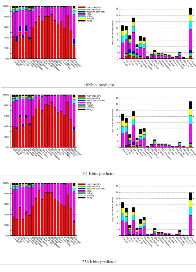
benchmark trace is illustrated in Mispredictions Per KiloInstructions (MPKI) on the right on Figures2 and3, (complete bar). It can be remarked that some benchmarks benefit a lot from the extra capacity of the large pre-dictor, while on some others, the fraction of branches that are intrinsically unpredictable by the TAGE predictor is large.

Confidence metrics In this paper, we are considering the confidence in a prediction family, i.e, for a given prediction, we are evaluating the probability of a misprediction. Since we will be manipulating probabilities ranging from very close to 0% and up to 40-50 %, we will measure misprediction rate in Misprediction per

KiloPredictions (MKP).

The metrics that were introduced by Grunwald et al [3], SENS, PVP, PVN, and SPEC are only suited for a binary discrimination of branches between high confidence and low confidence branches. In this paper we will consider up to 7 classes of branches. Therefore for a class of branches, we will use metrics more suited to any number of branch classes, the prediction coverage Pcov i.e. the fraction of branches that belong to this class, the misprediction coverage MPcov, i.e. the fraction of the all the mispredicted branches that belong to the class and

MPrate, the misprediction rate on the class (in MKP).

(10)

5 Confidence estimation by observation on the TAGE predictor

The TAGE predictor was shown to be very accurate and still represents the state-of-the-art on prediction accuracy at a fixed storage budget.

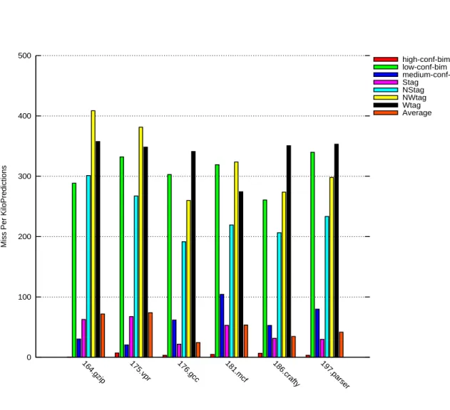
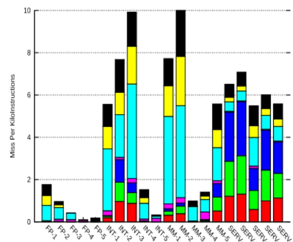
In this section, we show that by simply observing which component provides the prediction and the value of the prediction counter, one can obtain a very good estimation of the likelihood of a misprediction. We will show that up to 7 different classes of predictions with different confidence behaviors can be distinguished by simple observation.These classes will be described in the remainder of the section. Figures 2 and3 illustrate the coverage prediction coverage Pcov as well as the respective contribution in the overall misprediction rate (measured misprediction per kilo instructions) for each of these classes for the 3 predictor sizes and for each of the 40 traces. Figure4illustrate the misprediction rates MPrate for these 7 classes of branches for 7 benchmarks of CBP2 for the 64Kbits predictor.

5.1 The bimodal component as the provider component

For convenience, we will refer to the set of predictions provided by the bimodal component as the class BIM. The bimodal component provides the prediction when there is no hit on the tagged tables. On Figure2and3, the class

BIM corresponds to the three bottom components,high-conf-bim , medium-conf-bim and low-conf-bim. We will

explain later how we discriminate between low confidence , medium confidence and high confidence in the BIM class.

For the BIM class, the prediction coverage is generally quite significant (often more than 50 %) with 6% on INT-5 as a minimum to more than 80 % for some traces. At the same time, except for the CBP-1 server traces for the small predictor, the misprediction coverage for the bimodal component is significantly lower than its prediction coverage In practice, on the TAGE predictor, when the provider component is the bimodal component, this means that there has not been recently any mispredicted branch using the same PC address and history. On a very large predictor, a misprediction with the bimodal component as provider component should occur only during the warming phase of the predictor, therefore the misprediction rate for the predictions hitting on the bimodal component should be low.

5.1.1 Just considering the bimodal component origin

We measured the misprediction rate on the BIM prediction class provided by the bimodal component.

For the large 256Kbits predictor, 24 out of our 40 traces are exhibiting a misprediction rate lower than 1 MKP predictions on the BIM class.. The maximum misprediction rate that is encountered on the BIM class is 13 MKP on

INT2 while the overall misprediction rate on the complete application is 48 MKP. Therefore for the large predictor,

one can easily classify the predictions provided by the bimodal component as high confidence predictions. On the medium 64Kbits configuration, still 20 out of the 40 traces exhibit less than 1 MKP on the BIM class; however a few applications exhibit up a quite high misprediction rate on the BIM class. For instance MM-5 exhibits a 30 MKP misprediction rate on the BIM class which is still lower than its global misprediction rate (50 MKP), but is in the same range.

On the small 16Kbits configuration, 23 traces still exhibit insignificant misprediction rates (less than 3 MKP) on the BIM class. However due to aliasing on the bimodal predictor as well as limited capacity on the tagged components, some traces exhibit misprediction rates higher than 50 MKP, generally still lower than the mispre-diction rate on the rest of the premispre-dictions, but for some applications (e.g. the server traces) this mispremispre-diction rate is in the same range as the global misprediction rate (on SERV-2, 62 MKP on the BIM class and 59 MKP on average). Therefore, for the small predictor, classifying the predictions provided by the bimodal components as high confidence might be misleading for some applications.

This lead us to look for some way to discriminate among the predictions provided by the bimodal component.

5.1.2 Discriminating among the bimodal component mispredictions

We found two classes of predictions provided by the bimodal components that have a much higher misprediction rate than the average.

We illustrate this section with the average behavior on the CBP1 traces for the 16Kbits predictor and the 256Kbits predictor. For the 16Kbits (resp. 256Kbits) predictor, the bimodal component provides in average 50 %

(11)

8 Andr´e Seznec 0% 20% 40% 60% 80% 100%

FP-1FP-2FP-3FP-4FP-5INT-1INT-2INT-3INT-4INT-5MM-1MM-2MM-3MM-4MM-5SERV-1SERV-2SERV-3SERV-4SERV-5

high-conf-bim low-conf-bim medium-conf-bim Stag NStag NWtag Wtag 0 2 4 6 8 10

FP-1 FP-2 FP-3 FP-4 FP-5 INT-1 INT-2 INT-3 INT-4 INT-5 MM-1 MM-2 MM-3 MM-4 MM-5 SERV-1SERV-2SERV-3SERV-4SERV-5

Miss Per KiloInstructions

16Kbits predictor 0% 20% 40% 60% 80% 100%

64 Kbits predictor 0% 20% 40% 60% 80% 100%

256 Kbits predictor

Figure 2: Distribution of predictions (left) and distributions of mispredictions (right) for the CBP-1 traces.

(12)

0% 20% 40% 60% 80% 100%

164.gzip175.vpr176.gcc181.mcf186.crafty197.parser201.compress202.jess205.raytrace209.db213.javac222.mpegaudio227.mtrt228.jack252.eon253.perlbmk254.gap255.vortex256.bzip2300.twolf

high-conf-bim low-conf-bim medium-conf-bim Stag NStag NWtag Wtag 0 2 4 6 8 10 12 14 16

16Kbits predictor 0% 20% 40% 60% 80% 100%

64 Kbits predictor 0% 20% 40% 60% 80% 100%

256 Kbits predictor

(13)

10 Andr´e Seznec 0 100 200 300 400 500

164.gzip 175.vpr 176.gcc 181.mcf 186.crafty 197.parser

Miss Per KiloPredictions

high-conf-bim low-conf-bim medium-conf-bim Stag NStag NWtag Wtag Average

Figure 4: Misprediction rates per prediction class on 7 CBP2 traces, 64Kbits predictor

(14)

(resp. 45 %) of the predictions, 35 % (resp. 7 %) of the mispredictions and encounters an average misprediction rate of 29 MKP (resp. 3 MKP). The overall average misprediction rate is 40 MKP (resp. 28 MKP).

First as suggested by Smith [14] for the stand-alone bimodal predictor, when the prediction counter is weak, the prediction is not reliable at all. We will refer to this class of branches as the low-conf-bim class. Consistently, we observed a very high misprediction rate MPrate (30 % and above) on the low-conf-bim class. For the 16Kbits predictor (resp. 256Kbits) and on the CBP1 traces, low-conf-bim represents 3% (resp. 0.5 %) of the predictions in BIM but 32% (resp. 44 %) of the mispredictions in BIM. low-conf-bim exhibits an average misprediction rate of 317 MKP (resp. 448 MKP). Moreover in all cases where low-conf-bim constitute a substantial amount of the overall predictions (more than 1%), its misprediction rate exceeds 250 MKP (for INT3 on the 16Kbits predictor).. The low-conf-bim class can be classified as low confidence.

A second source of mispredictions in the BIM class is associated with the finite size of the predictor. Ideally, if the predictor had an infinite size, apart on the warming phase of the predictor, the bimodal component should provide the prediction only when the outcome of the (PC,history) pair is strongly biased towards the value of the bimodal counter. Unfortunately, the predictor has limited size and predictions on the tagged tables entries are overwritten in the predictor from time to time. Thus when the bimodal component is the provider of a mispre-diction, this might be an indication that the misprediction is due to a warming phase or some capacity issues in the predictor; capacity mispredictions are likely to occur in burst in a program. Simulations showed that indepen-dently of the size of the predictor, the predictions from the BIM class that occur just after a misprediction also in the BIM class (up to 8 branches in the illustrated experiments) are also quite likely generally a high probability to be mispredicted (in the range of 80-150 MKP for the 16Kbits predictor for CBP1). We refer to this class of predictions as the medium-conf-bim class. The prediction coverage of medium-conf-bim can be quite high on some benchmarks for the small TAGE predictor and much lower for the medium and large TAGE predictors. For the 16Kbits predictor (resp. 256Kbits) and on the CBP1 traces, medium-conf-bim represents 12 % (resp 1.5 %) of the predictions but 39% (resp. 24 %) of the mispredictions in BIM and exhibits an average misprediction rate of 87 MKP (resp. 57 MKP). This category of predictions can be classified as medium confidence.

The remainder of the predictions in BIM , i.e. the predictions with strong counters and distant from the last misprediction by the bimodal component exhibit a very low misprediction rate. We refer to this class of predictions as the high-conf-bim class. For the 16Kbits predictor (resp. 256Kbits) and on the CBP1 traces, high-conf-bim represents 85 % (resp. 98%) of the predictions and only 29 % (resp. 32 %) of the mispredictions in the BIM class and exhibits an average misprediction rate of only 9 MKP with a maximum of 21 MKP (resp. 1 MKP and a maximum of 5 MKP). This category of predictions can be classified as high confidence.

Therefore, through just observing its output, we can discriminate the predictions provided by the bimodal component in three separate classes of predictions that have very different probability of mispredictions. Note that as it could have been expected the medium confidence and low confidence predictions provided by the bimodal component nearly vanish on the large predictor.

5.2 Tagged components

In this section, we consider the predictions provided by the tagged components. We will discriminate among these predictions depending on the values of the prediction counter, more precisely on the absolute value of 2∗ ctr + 1 (to get a symmetry for positive and negative counters). We will refer to four classes defined respectively by|2 ∗ ctr + 1|=1 as the Wtag class (for weak counter), by |2 ∗ ctr + 1|=3 as the NWtag class (for nearly weak counter), by|2 ∗ ctr + 1|=5 as the NStag class (for nearly saturated counter) and by |2 ∗ ctr + 1|=7 as the Stag class (for saturated counter).

As was already pointed out in [13], the predictions in the Wtag class have a very high probabibility to be an incorrect prediction. This is not very surprising since a weak counter on a tagged component occurs only in the two following situations: either the entry has just been allocated after a misprediction or the counter has just been weakened or its sign flipped after providing a misprediction. It was observed that in that case the sign of the counter was leading to misprediction rates more than 40 % of the cases in average. The selective use of the alternate prediction described in Section3improves the quality of the branch prediction on this class of branches, but only in a limited way. On our benchmark set and for the three considered predictor configurations, the misprediction rate of the Wtag class is generally higher than 30 %.

As expected, the misprediction rate of the class decreases when the absolute value of the prediction counter increases. However this decrease is not so strongly marked, for instance on the 16Kbits (resp. 256Kbits) predictor and on CBP1, it decreases from 340 MKP (resp. 325 MKP) for Wtag, to 313 MKP (resp. 312 MKP) for NWtag, 213 MKP (resp. 225 MKP) for NStag and finally drops to 29 MKP (resp. 17 MKP) for the saturated counter class

(15)

12 Andr´e Seznec

NStag. Therefore despite predictions in the three non-saturated counter classes cover only a small fraction of the

predictions, e.g. 4.5 % (resp. 3.7 %) for the 16Kbits (resp. 256Kbits) predictor for the CBP1 traces, they cover a significant portion of the mispredictions, i.e., 32 % (resp 58 %) on the CBP1 traces. However it is noticeable that the saturated counter class Stag represents a sizeable portion of the predictions, 45 % (resp. 50 %) and presents a misprediction rate slightly lower than the average misprediction rate, but in the same range.

5.3 Partial summary

Up to now, by just examining the output of the TAGE predictor, we have been able to split the predictions in 7 classes that have quite different behaviors. Four of these classes, low-confid-bim, Wtag, NWtag, NStag , can be considered as low confidence (probability of a misprediction in the range of 200 MKP or higher) , 1 class,

high-confid-bim can be classified as very high confidence ( less than 10 MKP), 1 medium confidence class, medium-conf-bim and a last class, Stag i.e. saturated counters , which exhibits a misprediction rate close to the average

misprediction rate.

The saturated counter Stag is large. In average it covers about half of the predictions, and generally about one third of the mispredictions. In the next section, we show that a simple modification of the 3-bit counter automaton may allow to provide better confidence for Stag at the cost of reducing the size of the class and enlarging the NStag class.

6 Tweaking the 3-bit counter automaton

The 7 prediction classes presented above allows to discriminate between the branches. However in this classifi-cation, the saturated counter class Stag , is a good candidate as high confidence class for this classification for some traces, i.e. the applications with average misprediction rate in the 15 MKP range or less, but not for all applications. For instance on twolf, the misprediction rate on the Stag class is about 90 MKP. However a marginal modification of the 3-bit counter automaton for the tagged tables will allow us to discriminate the predictions in three classes, high confidence, medium confidence and low confidence.

Widening the prediction counter from 3 bits to 4 bits would create other classes of branches with slightly decreasing probability of mispredictions, but experiments showed tha would not significantly reduce the mispre-diction rate on the class of saturated counters, much wider counters would be needed; moreover widening the prediction counter has a slightly negative impact on the overall misprediction rate. Instead of widening the predic-tion counter, we propose to modify the saturated counter automaton in order to decrease the probability of reaching the saturated state as follows: On a correct prediction, whenever the counter is already equal to 2 or -3, the tran-sition to saturated state is only performed randomly with a small probability. Probability 1/128 is illustrated on Figure5and Figure6. That means that if the counter is saturated, then the probability that a misprediction has been provided by this counter in the recent past is very low.

Our experiments showed that such a modification of the 3-bit counter automaton increases the misprediction rate but only very marginally ( less than 0.02 misp/KI on our benchmark set in average). On the other hand, it allows to reduce the misprediction rate on the saturated counter class to a very low range in the order of 1-5 MKP: that is when the provider component is a tagged component and the counter is saturated then the prediction can be considered as high confidence.

At the same time, the NStag class (the nearly saturated counter class) is enlarged but its misprediction rate is significantly reduced. For instance on CBP1 and for the 16Kbits predictor, the saturated counter class Stag covers 27% of the predictions with a misprediction rate of 4 MKP while NStag covers 19% of the predictions with a misprediction rate of 67 MKP (against 40 MKP in average for all the predictions).

6.1 Towards three confidence classes of predictions

When the application is highly predictable, the high-conf-bim class and the saturated counter class Stag constitutes the vast majority of the predictions as can be observed for the 256Kbits predictor on CBP1 traces (Figure5). When the application has a quite high misprediction rate, the two intermediate classes NStag and low-bim-conf exhibiting a medium misprediction rate represents a significant fraction of the predictions and also of the mispredictions. This can be observed for the 16Kbits predictor for the server workload for low-bim-conf . NStag represents a significant part of the predictions for the intrinsically unpredictable benchmark like twolf, gzip, MM-1, MM-2 for instance.

(16)

0% 20% 40% 60% 80% 100%

16Kbits predictor, CBP1 0% 20% 40% 60% 80% 100%

64 Kbits predictor, CBP2 0% 20% 40% 60% 80% 100%

256 Kbits predictor, CBP1

Figure 5: Distribution of predictions (left) and distributions of mispredictions (right) , modified 3-bit counters automaton.

(17)

14 Andr´e Seznec 0 100 200 300 400 500

164.gzip 175.vpr 176.gcc 181.mcf 186.crafty 197.parser

Miss Per KiloPredictions

high-conf-bim low-conf-bim medium-conf-bim Stag NStag NWtag Wtag Average

Figure 6: Misprediction rates per prediction class on 7 CBP2 traces, 64Kbits predictor, modified 3-bit counter automaton

(18)

With this modified 3-bit counter automaton, we can divide the predictions in three classes with very different behaviors in terms of misprediction rates.

• Low confidence predictions include the weak bimodal counter class low-conf-bim and the weak and the nearly weak tagged counter classes Wtag and NWtag.

• Medium confidence predictions include the NStag class and the medium-conf-bim class predictions - i.e., predictions provided by the bimodal components in a warming phase or a capacity problem phase.

• High confidence prediction are the other predictions provided by the bimodal component i.e. the

high-conf-bim class and the saturated counter class Stag.

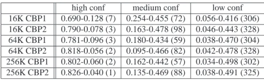
Table2 summarizes the coverage of branch predictions for respectively, high, medium and low confidence for the three predictor sizes and the two benchmark sets: first number represents the prediction coverage Pcov , second number is the misprediction coverage MPcov, and third number between parenthesis is the misprediction rate MPrate (in MKP).

It can be remarked that the high confidence prediction class covers the vast majority of the predictions and exhibits only a very small misprediction rate. Interestingly, the medium confidence predictions and the low confi-dence prediction covers both approximately half of the mispredictions, but with very different misprediction rates, typically more than 30 % for the low confidence branches and in the 5-15 % range for the medium confidence branches depending on the global misprediction rate of the application. Applications of branch confidence esti-mation can exploit this property as already suggested in [1] and in [8], for instance for controlling fetch gating or fetch throttling.

high conf medium conf low conf 16K CBP1 0.690-0.128 (7) 0.254-0.455 (72) 0.056-0.416 (306) 16K CBP2 0.790-0.078 (3) 0.163-0.478 (98) 0.046-0.443 (328) 64K CBP1 0.781-0.096 (3) 0.180-0.434 (59) 0.038-0.470 (304) 64K CBP2 0.818-0.056 (2) 0.095-0.466 (82) 0.042-0.478 (328) 256K CBP1 0.802-0.060 (2) 0.162-0.442 (57) 0.034-0.498 (302) 256K CBP2 0.826-0.040 (1) 0.135-0.469 (88) 0.038-0.491 (325)

Table 2: Prediction and misprediction coverages, misprediction rates (in MKP) for high, medium and low confi-dence prediction classes

6.2 Varying the saturated counter reaching probability

In the illustrated experiments, we used 1/128 as the probability for saturating the 3-bit counter. Using a smaller probability e.g. 1/16 would increase the coverage of the Stag class at the cost of an increase of misprediction coverage and its misprediction rate. For instance on the 16Kbits predictor, the prediction coverage of the high confidence class reaches 79 % (against 69 % when using 1/128) while its misprediction rate grows to 10 MKP instead of 7 MKP and its misprediction coverage grows to 22,3 % instead of 12,8 %.

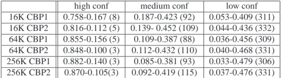
This probability can also be adapted at run-time in order to meet some desired characteristics. For instance, we implemented an adaptive probability algorithm (varying from 1/1024 to 1 by multiplication/division factor of 2). The algorithm monitors the misprediction rate of the high-confidence predictions and tries to maximizes the coverage of the high-confidence class but dynamically maintains the misprediction rate on the class under 10 MKP. Table3summarizes the results for this experiment.

7 Conclusion

Confidence estimation of branch predictions has been shown to be useful for several usages in microarchitecture e.g. fetch gating or fetch throttling for energy saving, SMT fetch policy for resource balancing among threads. Most studies on confidence estimation usage have been considering branch predictors that were defined in the 90’s and have considered only two classes of branches: high confidence and low confidence. More recent studies [1,8]

(19)

16 Andr´e Seznec

high conf medium conf low conf 16K CBP1 0.758-0.167 (8) 0.187-0.423 (92) 0.053-0.409 (311) 16K CBP2 0.816-0.112 (5) 0.139- 0.452 (109) 0.044-0.436 (332) 64K CBP1 0.855-0.156 (5) 0.109-0.387 (88) 0.036-0.456 (309) 64K CBP2 0.848-0.100 (3) 0.112-0.432 (110) 0.040-0.468 (331) 256K CBP1 0.882-0.140 (3) 0.085-0.381 (93) 0.033-0.479 (306) 256K CBP2 0.870-0.105(3) 0.092-0.419 (115) 0.037-0.476 (331)

Table 3: Prediction and misprediction coverages, misprediction rates for high, medium and low confidence pre-diction classes, adaptive probability used to maintain MPrate < 10 MKP on high confidence prepre-diction

have shown that it might be useful to consider a wider spectrum of confidence classes. All these studies generally consider confidence estimators requiring storage tables.

In this paper, we have shown that accurate confidence estimation for the state-of-the-art branch predictor, TAGE does not require complex hardware or a lot of extra storage. Confidence in a branch prediction can be obtained through the observation of the outputs of the predictor components. 7 classes of predictions with different confidence behaviors can be observed. Moreover, we have shown that a simple modification of the 3-bit counter automaton used in the tagged components of the TAGE predictor allows to split the predictions in three confidence classes with very distinct behavior, the high confidence prediction class with misprediction rate lower than 1%, the medium confidence class with misprediction rate in the 8%-12% misprediction rate and the low confidence prediction class with misprediction rate higher than 30 %.

Acknowledgement

This research was partially supported by an Intel Research Grant.

References

[1] H. Akkary, S. T. Srinivasan, R. Koltur, Y. Patil, and W. Refaai. Perceptron-based branch confidence estima-tion. In HPCA, pages 265–275, 2004.

[2] J. L. Aragón, J. González, and A. González. Power-aware control speculation through selective throttling. In HPCA, pages 103–112, 2003.

[3] D. Grunwald, A. Klauser, S. Manne, and A. Pleszkun. Confidence estimation for speculation control. In

ISCA ’98: Proceedings of the 25th annual international symposium on Computer architecture, pages 122–

131, Washington, DC, USA, 1998. IEEE Computer Society.

[4] E. Jacobsen, E. Rotenberg, and J. E. Smith. Assigning confidence to conditional branch predictions. In

MICRO, pages 142–152, 1996.

[5] D. Jimenez and C. Lin. Composite confidence estimators for enhanced speculation control. Technical report tr 02-14, University of Texas at Austin, 2002.

[6] A. Klauser, A. Paithankar, and D. Grunwald. Selective eager execution on the polypath architecture. In

ISCA, pages 250–259, 1998.

[7] K. Luo, M. Franklin, S. S. Mukherjee, and A. Seznec. Boosting smt performance by speculation control. In

IPDPS, page 2, 2001.

[8] K. Malik, M. Agarwal, V. Dhar, and M. I. Frank. Paco: Probability-based path confidence prediction. In

HPCA, pages 50–61, 2008.

[9] S. Manne, A. Klauser, and D. Grunwald. Branch prediction using selective branch inversion. In IEEE PACT, pages 48–56, 1999.

(20)

[10] S. McFarling. Combining branch predictors. TN 36, DEC WRL, June 1993.

[11] A. Seznec. Analysis of the o-gehl branch predictor. In Proceedings of the 32nd Annual International

Symposium on Computer Architecture, june 2005.

[12] A. Seznec. The l-tage branch predictor. Journal of Instruction Level Parallelism (http://www.jilp.org/vol9), April 2006.

[13] A. Seznec and P. Michaud. A case for (partially)-tagged geometric history length predictors. Journal of

Instruction Level Parallelism (http://www.jilp.org/vol8), April 2006.

[14] J. Smith. A study of branch prediction strategies. In Proceedings of the 8th Annual International Symposium

on Computer Architecture, 1981.

[15] H. Vandierendonck and A. Seznec. Fetch gating control through speculative instruction window weighting. In HiPEAC, pages 120–135, 2007.

(21)

Centre de recherche INRIA Rennes – Bretagne Atlantique IRISA, Campus universitaire de Beaulieu - 35042 Rennes Cedex (France)

Centre de recherche INRIA Bordeaux – Sud Ouest : Domaine Universitaire - 351, cours de la Libération - 33405 Talence Cedex Centre de recherche INRIA Grenoble – Rhône-Alpes : 655, avenue de l’Europe - 38334 Montbonnot Saint-Ismier Centre de recherche INRIA Lille – Nord Europe : Parc Scientifique de la Haute Borne - 40, avenue Halley - 59650 Villeneuve d’Ascq

Centre de recherche INRIA Nancy – Grand Est : LORIA, Technopôle de Nancy-Brabois - Campus scientifique 615, rue du Jardin Botanique - BP 101 - 54602 Villers-lès-Nancy Cedex

Centre de recherche INRIA Paris – Rocquencourt : Domaine de Voluceau - Rocquencourt - BP 105 - 78153 Le Chesnay Cedex Centre de recherche INRIA Saclay – Île-de-France : Parc Orsay Université - ZAC des Vignes : 4, rue Jacques Monod - 91893 Orsay Cedex

Centre de recherche INRIA Sophia Antipolis – Méditerranée : 2004, route des Lucioles - BP 93 - 06902 Sophia Antipolis Cedex

Éditeur

INRIA - Domaine de Voluceau - Rocquencourt, BP 105 - 78153 Le Chesnay Cedex (France)

http://www.inria.fr