HAL Id: hal-00667583
https://hal.archives-ouvertes.fr/hal-00667583
Submitted on 8 Feb 2012
HAL is a multi-disciplinary open access
archive for the deposit and dissemination of
sci-entific research documents, whether they are
pub-lished or not. The documents may come from
teaching and research institutions in France or
abroad, or from public or private research centers.
L’archive ouverte pluridisciplinaire HAL, est
destinée au dépôt et à la diffusion de documents
scientifiques de niveau recherche, publiés ou non,
émanant des établissements d’enseignement et de
recherche français ou étrangers, des laboratoires
publics ou privés.
Pose and Expression-Invariant 3D Face Recognition
using Elastic Radial Curves
Hassen Drira, Boulbaba Ben Amor, Mohamed Daoudi, Anuj Srivastava
To cite this version:
Hassen Drira, Boulbaba Ben Amor, Mohamed Daoudi, Anuj Srivastava. Pose and Expression-Invariant
3D Face Recognition using Elastic Radial Curves. British machine vision conference, Aug 2010,
Aberystwyth, United Kingdom. pp.1-11. �hal-00667583�
Pose and Expression-Invariant 3D Face
Recognition using Elastic Radial Curves
Hassen Drira1
http://www.telecom-lille1.eu/people/drira Boulbaba Ben Amor12
http://www.telecom-lille1.eu/people/benamor Mohamed Daoudi12 http://www.telecom-lille1.eu/people/daoudi Anuj Srivastava3 http://stat.fsu.edu/~anuj/ 1LIFL (UMR CNRS 8022), University of Lille 1, Villeneuve d’Ascq, France. 2TELECOM Lille 1 ;
Institut TELECOM, France. 3Department of Statistics,
Florida State University, Florida, USA.
Abstract
In this paper we explore the use of shapes of elastic radial curves to model 3D facial deformations, caused by changes in facial expressions. We represent facial surfaces by indexed collections of radial curves on them, emanating from the nose tips, and com-pare the facial shapes by comparing the shapes of their corresponding curves. Using a past approach on elastic shape analysis of curves, we obtain an algorithm for comparing facial surfaces. We also introduce a quality control module which allows our approach to be robust to pose variation and missing data. Comparative evaluation using a com-mon experimental setup on GAVAB dataset, considered as the most expression-rich and noise-prone 3D face dataset, shows that our approach outperforms other state-of-the-art approaches.
1
Introduction and related work
A biometric-based recognition system can be very useful in a variety of applications. While some biometric modalities, such as fingerprints and iris, have already reached very high level of accuracy, they have a limited use in non-cooperative scenarios. On the other hand, the less-intrusive modalities like the face and gait have not reached the desired levels of accuracy. Over the past three decades, the techniques for face recognition have received a growing attention within the computer vision community. Within this problem area, the 2-D and 3-D data represent the two different kinds of challenges.
We can classify existing 3D face recognition methods into two categories. First, some methods, such as Moussavi et al. [11], Mahoor et al. [9] and Li et al.[8], are interested in adopting low-level geometric features to face recognition for several reasons. They claim that they spend less effort in extracting features unlike the methods that are based on extract-ing high-level geometric features, e.g., shapes of facial curves [13], concave and convex facial regions [1], partial face regions [5][10], or deformation distance metrics [7]. The latest methods constitute the second category, and their recognition performance generally
c
2010. The copyright of this document resides with its authors. It may be distributed unchanged freely in print or electronic forms.
depends on the reliability of the feature. For this reason, it is necessary to spend effort to extract these features and look for elaborate tools to compare them. For example, shape anal-ysis can be a good candidate especially it has shown good performance in previous works [13]. Our approach is to represent facial surfaces as indexed collections of radial curves in order to handle pose and expression variations. The main differences between this work and previous curve-based approaches are as follows. Samir et al. [13] used the level curves of the height function to define facial curves. Since these curves are planar, they used shape anal-ysis of planar curves to compare faces; non-linear matching problem was not studied here (that is, the mapping between curves was fixed to be linear). The metric used was a non-elastic metric and the shooting method was used for computing geodesics between planar curves. Consequently, this representation is not fully invariant to rigid motions of the face. In [14], the level curves of the surface distance function that resulted in 3D curves are used. The authors used a non-elastic metric and a path-straightening method to compute geodesics between these curves. Here also the matching was not studied and the correspondence of curves and points across faces was simply linear. However, the open mouth corrupts the shape of some level curves and this parameterization does not handle this problem. To avoid this problem of open mouth, Drira et al. [4] proposed partial biometrics. That is, they studied the contribution of only the nose region in 3D face recognition using a similar level curve based approach. They used elastic matching for curves comparison. Mpiperis et al. [12] proposed a geodesic polar parameterization of the face surface. With this parameterization, the intrinsic surface attributes do not change under isometric deformations when the mouth is closed. When the mouth is open it violates the isometric assumption and they modify their geodesic polar parameterization by disconnecting the lips. Therefore, their approach requires lips detection [3]. In [2] and [1] Berretti et al. proposed to use features derived from the surface paths around the nose. In [2], the radial curves were extracted as features, then matched using SVM classifiers. Experimental results on GAVAB dataset shows that this approach is sensitive to expression variations. (Rank one recognition rate = 75.4% for non-neutral expressions). In [1], a compact graph representation is constructed for each face. In this way, the structural similarity between two face models is evaluated by matching their corresponding graphs.
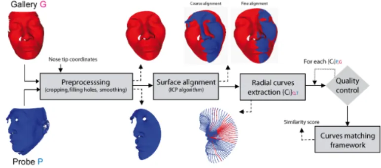
Figure 1: Overview of the proposed method.
In this paper, we extract radial curves as features (in a similar way than [2] and [12]). However, we apply elastic shape analysis in order to keep the intrinsic surface attributes under isometric deformations even when the mouth is open. In other words, our choice of representation is based on ideas followed previously in [14] but using a collection of
radial curves to represent a surface and not iso-curves. Our contribution in this paper is an extension of the previous elastic shape analysis framework [6] of opened curves to surfaces which is able to model facial deformations dues to expressions, even with an open mouth face. We demonstrate the effectiveness of our approach by comparing the state of the art results. However, unlike previous works dealing with large facial expressions, especially when the mouth is open [12][3] which require lips detection, our approach mitigates this problem without any lip detection. Indeed, besides the modeling of elastic deformations, the proposed shape analysis-based framework solves the problem of opening of the mouth without any need to detect lip contours as in [12] and [3]. Figure2 illustrates the overall proposed 3D face recognition method. First of all, the probe P and the gallery G meshes are preprocessed. This step is essential to improve the quality of raw images and to extract the useful part of the face. It consists of a Laplacian smoothing filter to reduce the acquisition noise, a filling hole filter that identifies and fills holes in input mesh, and a cropping filter that cuts and returns the part of the input mesh inside of a specified sphere. Then, a coarse alignment is performed based on the translation vector formed by the tips of the noses. This step is followed by a finer alignment based on the well-known ICP algorithm in order to normalize the pose. Next, we extract the radial curves emanating from the nose tip and having different directions on the face. Within this step, a quality control module inspects the quality of each curve on both meshes and keeps only the good ones based on defined criteria.
In order to improve matching and comparisons between the extracted curves, we advo-cate the use of elastic matching. Actually, facial deformations dues to expressions can be attenuated by an elastic matching between facial curves. Hence, we obtain algorithm for computing geodesics between pair wise of radial curves on gallery and probe meshes. The length of one geodesic measures the degree of similarity between one pair of curves. The fusion of the scores on good quality common curves, produced similarity score between the faces P and G. We detail the pipeline of all these stages contained in our method in the fol-lowing sections. Section 3 describes surface preprocessing and alignment steps. In Section 4 we explain the radial curves extraction step and focus on the quality control module. Sec-tion 5 presents the Riemannian framework to analyze shapes of curves and its extension to compare facial surfaces. We demonstrate in section 6 the performance to recognize people in presence of both expression and pose variations. The section 7 suggests some future work and provide some concluding remarks.
2
Preprocessing and surfaces alignment
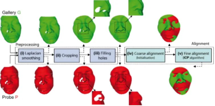
As illustrated in Figure2, we start by preprocessing the input raw images in order to im-prove their quality. Indeed, these images present some imperfections as holes, spikes and includes some undesired parts (clothes, neck, ears, hair, etc.) and so on. This step consists of a pipeline of 3D mesh processing filters. (i) Smoothing filter reduces high frequency infor-mation (spikes) in the geometry of the mesh, making the cells better shaped and the vertices more evenly distributed. (ii) Cropping filter cuts and returns parts of the mesh inside a de-fined implicit function. This function is a sphere dede-fined by the nose tip as its center and the radius 75mm in order to avoid as much hair. (iii) Filling holes filter identifies and fills holes in input meshes. Holes are created either because of the absorption of laser in dark areas such as eyebrows and mustaches, occlusion or mouth opening. They are identified in the input mesh by locating boundary edges, linking them together into loops, and then
trian-gulating the resulting loops. After meshes preprocessing, we correct their poses to properly compare the faces by establishing correct correspondence between sets of curves of probe and gallery images. (iv) Coarse alignment filter fixes the probe image P onto the Gallery image G at the nose tip. In other words, this filter performs a translation transform along the vector defined by the two tips of the noses. This step presents a good initialization to the (v)
Fine alignment filterwhich performs ICP algorithm on obtained meshes. The fine alignment filter also corrects non-frontal meshes to make them frontal.
Figure 2: Pipline of preprocessing filters and alignment procedure.
3
Radial curves extraction and quality control
Our recognition approach is based on elastic matching of radial curves extracted from facial surfaces. After preprocessing and alignment stages, we represent each facial surface by an indexed collection of radial curves emanating from the nose tips. To address the missing data and large pose variations, we introduce a quality control module that inspects the quality of extracted curves and remove bad quality ones.
3.1
Radial curves extraction
Now we introduce our mathematical representation of a facial surface. Let S be a facial surface denoting the output of the previous preprocessing step. Although S is a triangulated mesh, we start the discussion by assuming that it is a continuous surface. Letβαdenote the
radial curve on S which makes an angleα with a reference radial curve. The reference curve is chosen to be the vertical curve once the face has been rotated to the upright position. In practice, each radial curveβα is obtained by slicing the facial surface by a plane Pα that
has the nose tip as its origin and makes an angleα with the plane containing the reference curve. That is, the intersection of Pα with S givesβα. We repeat this step to extract radial
curves from the facial surface at equal angular separation. If needed, we can approximately reconstruct S from these radial curves according to S≈ ∪αβα= ∪α{S ∩ Pα} as illustrated in
Figure3. This indexed collection of radial curves captures the shape of a facial surface and forms our mathematical representation of that surface. We have chosen to represent a surface with a collection of curves since we have better tools for elastically analyzing shapes of curves than we have for surfaces. More specifically, we are going to utilize an elastic method
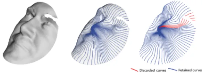
for studying shapes of curves that is especially suited to modeling deformations associated with changes in facial expressions. Notice that some curves can reduce the performance of the algorithm as they have bad quality. These curves should be, first, detected and then removed. In figure3, we show the result of curves extraction and we show only curves that have passed the quality filter. We give further details about that filtering next.
3.2
Quality filter for curves selection
This filter is applied on the curves after the face preprocessing step. Actually, these curves are considered as features of the face and the distance between faces is based on these curves. The aim of that filter is to remove curves which have bad quality. To pass the quality filter, a curve should be continuous and having a minimum of length. The discontinuity or a shortness of a curve results from the missing data on the face or presence of large noise. To illustrate this idea, we show in figure3an example of extracted curves on a face and then the result of quality filter on these curves. Once the quality of the features is controlled, we proceed to faces comparison.
Figure 3: Radial curves extraction and quality filter application.
In the following sections we describe our framework to analyze shape of curves in order to compare the selected features.
4
Facial surfaces comparisons
Let β : I→ R3, for I= [0,1], represent a facial curve generated as described above. To
analyze the shape of β , we shall represent it mathematically using a square-root velocity
function(SRVF), denoted by q(t), according to:
q(t) .=qβ˙(t) k ˙β(t)k
. (1)
q(t) is a special function introduced by [6] that captures the shape ofβ and is particularly convenient for shape analysis. It has been shown in [6] that the classical elastic metric for comparing shapes of curves becomes the L2-metric under the SRVF representation. This point is very important as it simplifies the calculus of elastic metric to the well-known cal-culus of functional analysis under the L2-metric. We define the set:
With the L2metric on its tangent spaces, C becomes a Riemannian manifold. In particu-lar, since the elements of C have a unit L2norm, C is a hypersphere in the Hilbert space L2(I,R3). In order to compare the shapes of two radial curves, we can compute the distance between them in C under the chosen metric. This distance is defined to be the length of the (shortest) geodesic connecting the two points in C . Since C is a sphere, the formulas for the geodesic and the geodesic length are already well known. The geodesic length between any two points q1,q2∈ C is given by:
dc(q1,q2) = cos
−1(hq
1,q2i), (3) and the geodesic pathα :[0,1] → C , is given by:
α(τ) = 1
sin(θ )(sin((1 − τ)θ )q1+ sin(θ τ)q2), whereθ= dc(q1,q2).
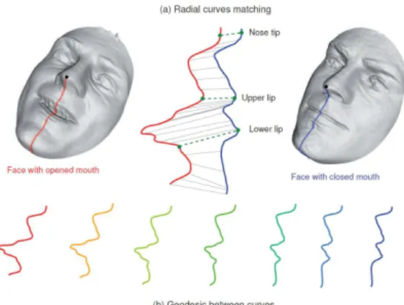
Figure 4: Matching and geodesic deforming radial curves in presence of expressions.
It is easy to see that several elements of C can represent curves with the same shape. For example, if we rotate a face in R3, and thus its facial curves, we get different SRVFs
for the curves but their shapes remain unchanged. Another similar situation arises when a curve is re-parametrized; a re-parameterization changes the SRVF of curve but not its shape. In order to handle this variability, we define orbits of the rotation group SO(3) and the re-parameterization group Γ as equivalence classes in C . Here, Γ is the set of all orientation-preserving diffeomorphisms of I (to itself) and the elements of Γ are viewed as re-parameterization functions. For example, for a curveβ : I→ R3and a functionγ ∈ Γ,
the curveβ◦ γ is a re-parameterization of β . The corresponding SRVF changes according to
q(t) 7→p ˙γ(t)q(γ(t)). We define the equivalent class containing q as: [q] = {p ˙γ(t)Oq(γ(t))|O ∈ SO(3), γ∈ Γ},
The set of such equivalence class is called the shape space S of elastic curves [6]. To obtain geodesics and geodesic distances between elements of S , one needs to solve the op-timization problem, which is typically done using dynamic programming. An example of
this idea is shown in Figure4, where we take two radial curves from two faces and compute a geodesic path between them in S . The middle panel in the top row shows the optimal matching for the two curves obtained using the dynamic programming, and this highlights the elastic nature of this framework. For the left curve, the mouth is open and for the right curve, it is closed. Still the feature points (upper and bottom lips) match each other very well. The bottom row shows the geodesic path between the two curves in the shape space S and this evolution looks very natural under the elastic matching. Since we have geodesic paths denoting optimal deformations between individual curves, we can combine these de-formations to obtain full dede-formations between faces.
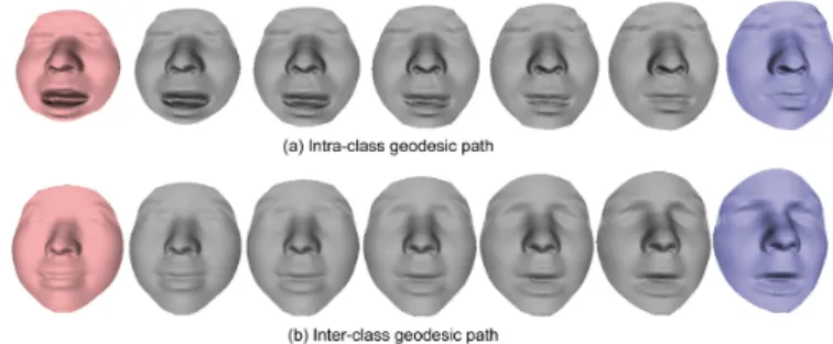
In fact, these full deformations are geodesic paths between faces when represented as elements of S[0,α0]. Shown in Figure5are examples of such geodesic paths between source and target faces. It is clear that the geodesic in the shape space models in a natural way the deformation from the source to the target, especially in mouth region. We present the illustrations in both cases; case of inter-class path (source and target belong to different persons) and intra-class path (source and target belong to the same person).
Figure 5: Examples of intra-class geodesic (top row), and inter-class geodesic (lower row).
5
Evaluation
The proposed approach for representation and matching of faces has been evaluated using the GavabDB database. We first describe the experimental setup. Then, we test our recognition method, discuss the results and give comparisons with state of the art approaches. Table5
present the Time Consumed for different steps of our algorithm on a PC with a 3 Ghz Core 2 Duo processor with 3 GB memory.
Table 1: Computational cost
Step Time consumed (s)
Mesh Preprocessing 0.375 (per face)
Mesh Alignment 0.125
Curves extraction 0.485 (all curves, 2 faces) Quality control 0.000001875 (per curve) Curve preprocessing 0.137 (per curve)
Curve comparison 0.0318 (per curve)
5.1
The dataset
To the best of our knowledge, GavabDB is the most expression-rich and noise-prone 3D face dataset currently available to the public. The GavabDB consists of Minolta Vi-700 laser range scans from 61 different subjects. The subjects, of which 45 are male and 16 are female, are all Caucasian. Each subject was scanned 9 times for different poses and expressions, namely six neutral expression scans and three scans with an expression. The neutral scans include two different frontal scans, one scan while looking up (+35 degree), one scan while looking down (-35 degree), one scan from the right side (+90 degree), and one from the left side (-90 degree). The expression scans include one with a smile, one with a pronounced laugh, and an arbitrary expression freely chosen by the subject [15]. Figure6
shows some examples of faces in this dataset.
Figure 6: Examples of all 3D scans of the same subject from GAVAB dataset.
5.2
Experimental results
In order to assess the effectiveness of the proposed solution for face identification, we per-formed extensive experiments. In these experiments, one of the two frontal models with the neutral expression provided for each person is taken as a gallery model for the identification.
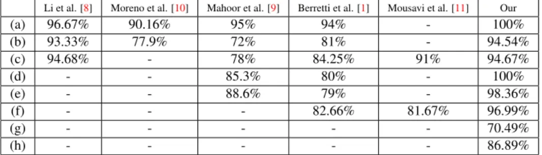
Table 2: Comparison of recognition rates using different methods : (a) Neutral, (b) Expressive, (c) Neutral+expressive, (d) Rotated looking down, (e) Rotated looking up, (f) Overall, (g) Scans from right sight, (g) Scans from left sight.
Li et al. [8] Moreno et al. [10] Mahoor et al. [9] Berretti et al. [1] Mousavi et al. [11] Our
(a) 96.67% 90.16% 95% 94% - 100% (b) 93.33% 77.9% 72% 81% - 94.54% (c) 94.68% - 78% 84.25% 91% 94.67% (d) - - 85.3% 80% - 100% (e) - - 88.6% 79% - 98.36% (f) - - - 82.66% 81.67% 96.99% (g) - - - 70.49% (h) - - - 86.89%
Table2illustrates the results of the matching accuracy for different categories of probe faces. We notice that the proposed approach provides a high recognition accuracy for ex-pressive faces (94.54%). This is due to both face parameterization using radial curves and elastic matching techniques. Actually, each curve represents a feature that caracterizes a lo-cal region in the face contrary to the using closed level curves. Besides, the elastic matching is able to establish a correspondence with guaranteed alignment among anatomical facial features. Figure4shows an example of matching lower lips of the mouth together and also
upper lips, although a large deformation in one face due to the opening of the mouth. Figure
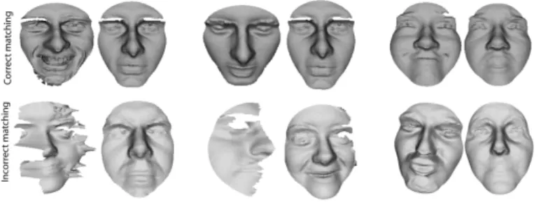
7 (top row) illustrates some recognition examples of expressive and pose modified probe faces. For each case, on the left the probe face is shown, while on the right the correctly identified reference face (gallery) is reported. These models also provide examples of the variability in terms of facial expression of face models included in the probe dataset. As far as neutral expressions are concerned, the accuracy depends on the pose. We correct the pose using one iteration of ICP algorithm as the poses are very difficult. Actually, the accuracy is not affected when the pose is frontal or rotated looking down (the recognition rate is 100%).
Figure 7: Recognition examples. For each pair, the probe (on the left) and the retrieved (on the left) faces are reported.
We can see in figure7(top row) an examples of well matched faces although its pose (looking down). However, the accuracy is no more perfect but still very high (98.36%) for the looking up pose. According to scans from right and left sides, the accuracy is not very high as missing data are very important. Figure7(lower row) illustrates some bad matchings. For each pair, the probe (on the left), the first closest face (on the left) are reported. To the best of our knowledge, no earlier work included scans from left and right sights in their experimental protocol when using GAVAB dataset. Therefore, we show in table2comparison with other methods on a subset of GAVAB dataset (without these scans). Notice that the experimental protocol is the same; one of the two frontal neutral scan is choosen as gallery, remaining faces constitute the probe dataset. As shown in the table, our method outperforms all other ones in terms of recognition rates.
6
Conclusion and Perspectives
In this paper we have proposed an original solution to the problem of 3D face recognition. We have illustrated a geometric analysis of 3D facial shapes in presence of both facial ex-pressions and pose variations. The key idea here is the representation of a face by its radial curves, and the comparisons of those radial curves using the elastic shape analysis. We re-ported results on GAVAB dataset and our result outperforms previous works on that dataset. Future work will address more importance to automatically nose tip detection when the pose is not frontal and also to the way of fusion the scores emaning from each feature.
Acknowledgements
This research is supported in part by the ANR under the project ANR-07-SESU-004 and the Contrat de Projet Etat-Région (CPER) Région Nord-Pas de Calais Ambient Intelligence and partially supported by the following grants : ARO W911NF-04-01-0268 and AFOSR FA9550-06-1-0324 to Anuj Srivastava. Additionally, Anuj Srivastava was supported by vis-iting professorships from University of Lille I and CNRS in summers of 2007-2009.
References
[1] Stefano Berretti, Alberto Del Bimbo, and Pietro Pala. 3d face recognition by modeling the arrangement of concave and convex regions. In Adaptive Multimedia Retrieval, pages 108–118, 2006.
[2] Stefano Berretti, Alberto Del Bimbo, Pietro Pala, and Francisco Silva-Mata. Face recognition by svms classification of 2d and 3d radial geodesics. In ICME, pages 93– 96, 2008.
[3] Alexander M. Bronstein, Michael M. Bronstein, and Ron Kimmel. Expression-invariant representations of faces. IEEE Transactions on Image Processing, 16(1): 188–197, 2007.
[4] Hassen Drira, Boulbaba Ben Amor, Anuj Srivastava, and Mohamed Daoudi. A rieman-nian analysis of 3d nose shapes for partial human biometrics. In IEEE International
Conference on Computer Vision, pages 2050–2057, 2009.
[5] Timothy C. Faltemier, Kevin W. Bowyer, and Patrick J. Flynn. A region ensemble for 3-d face recognition. IEEE Transactions on Information Forensics and Security, 3(1): 62–73, 2008.
[6] Shantanu H. Joshi, Eric Klassen, Anuj Srivastava, and Ian Jermyn. A novel represen-tation for riemannian analysis of elastic curves in rn. In CVPR, 2007.
[7] I. A. Kakadiaris, G. Passalis, G. Toderici, M. N. Murtuza, Y. Lu, N. Karampatziakis, and T. Theoharis. Three-dimensional face recognition in the presence of facial ex-pressions: An annotated deformable model approach. IEEE Transactions on Pattern
Analysis and Machine Intelligence, 29(4):640–649, 2007.
[8] Xiaoxing Li, Tao Jia, and Hao Zhang. Expression-insensitive 3d face recognition using sparse representation. Computer Vision and Pattern Recognition, IEEE Computer
So-ciety Conference on, 0:2575–2582, 2009. doi: http://doi.ieeecomputersociety.org/10. 1109/CVPRW.2009.5206613.
[9] Mohammad H. Mahoor and Mohamed Abdel-Mottaleb. Face recognition based on 3d ridge images obtained from range data. Pattern Recognition, 42(3):445–451, 2009. [10] Ana Belen Moreno, Angel Sanchez, Jose Fco. Velez, and Fco. Javier Díaz. Face
recog-nition using 3d local geometrical features: Pca vs.svm. In Int. Symp. on Image and
[11] Mir Hashem Mousavi, Karim Faez, and Amin Asghari. Three dimensional face recog-nition using svm classifier. In ICIS ’08: Proceedings of the Seventh IEEE/ACIS
Inter-national Conference on Computer and Information Science (icis 2008), pages 208–213, Washington, DC, USA, 2008. IEEE Computer Society. ISBN 978-0-7695-3131-1. doi: http://dx.doi.org/10.1109/ICIS.2008.77.
[12] Iordanis Mpiperis, Sotiris Malassiotis, and Michael G. Strintzis. 3-d face recognition with the geodesic polar representation. IEEE Transactions on Information Forensics
and Security, (3-2):537–547.
[13] Chafik Samir, Anuj Srivastava, and Mohamed Daoudi. Three-dimensional face recognition using shapes of facial curves. IEEE Transactions on Pattern Analy-sis and Machine Intelligence, 28:1858–1863, 2006. ISSN 0162-8828. doi: http: //doi.ieeecomputersociety.org/10.1109/TPAMI.2006.235.
[14] Chafik Samir, Anuj Srivastava, Mohamed Daoudi, and Eric Klassen. An intrinsic framework for analysis of facial surfaces. International Journal of Computer Vision, 82(1):80–95, 2009.
[15] Frank B. ter Haar, Mohamed Daoudi, and Remco C. Veltkamp. Shape retrieval contest 2008: 3d face scans. Shape Modeling and Applications, International Conference on, 0:225–226, 2008. doi: http://doi.ieeecomputersociety.org/10.1109/SMI.2008.4547979.