Regularized LIML for many instruments

Texte intégral

(1)2013s-20. Regularized LIML for many instruments Marine Carrasco, Guy Tchuente. Série Scientifique Scientific Series. Montréal Juillet 2013. © 2013 Marine Carrasco, Guy Tchuente. Tous droits réservés. All rights reserved. Reproduction partielle permise avec citation du document source, incluant la notice ©. Short sections may be quoted without explicit permission, if full credit, including © notice, is given to the source..

(2) CIRANO Le CIRANO est un organisme sans but lucratif constitué en vertu de la Loi des compagnies du Québec. Le financement de son infrastructure et de ses activités de recherche provient des cotisations de ses organisations-membres, d’une subvention d’infrastructure du Ministère du Développement économique et régional et de la Recherche, de même que des subventions et mandats obtenus par ses équipes de recherche. CIRANO is a private non-profit organization incorporated under the Québec Companies Act. Its infrastructure and research activities are funded through fees paid by member organizations, an infrastructure grant from the Ministère du Développement économique et régional et de la Recherche, and grants and research mandates obtained by its research teams. Les partenaires du CIRANO Partenaire majeur Ministère de l'Enseignement supérieur, de la Recherche, de la Science et de la Technologie Partenaires corporatifs Autorité des marchés financiers Banque de développement du Canada Banque du Canada Banque Laurentienne du Canada Banque Nationale du Canada Banque Scotia Bell Canada BMO Groupe financier Caisse de dépôt et placement du Québec Fédération des caisses Desjardins du Québec Financière Sun Life, Québec Gaz Métro Hydro-Québec Industrie Canada Investissements PSP Ministère des Finances et de l’Économie Power Corporation du Canada Rio Tinto Alcan State Street Global Advisors Transat A.T. Ville de Montréal Partenaires universitaires École Polytechnique de Montréal École de technologie supérieure (ÉTS) HEC Montréal Institut national de la recherche scientifique (INRS) McGill University Université Concordia Université de Montréal Université de Sherbrooke Université du Québec Université du Québec à Montréal Université Laval Le CIRANO collabore avec de nombreux centres et chaires de recherche universitaires dont on peut consulter la liste sur son site web. Les cahiers de la série scientifique (CS) visent à rendre accessibles des résultats de recherche effectuée au CIRANO afin de susciter échanges et commentaires. Ces cahiers sont écrits dans le style des publications scientifiques. Les idées et les opinions émises sont sous l’unique responsabilité des auteurs et ne représentent pas nécessairement les positions du CIRANO ou de ses partenaires. This paper presents research carried out at CIRANO and aims at encouraging discussion and comment. The observations and viewpoints expressed are the sole responsibility of the authors. They do not necessarily represent positions of CIRANO or its partners.. ISSN 1198-8177. Partenaire financier.

(3) Regularized LIML for many instruments * Marine Carrasco †, Guy Tchuente ‡. Résumé / Abstract The use of many moment conditions improves the asymptotic efficiency of the instrumental variables estimators. However, in finite samples, the inclusion of an excessive number of moments increases the bias. To solve this problem, we propose regularized versions of the limited information maximum likelihood (LIML) based on three different regularizations: Tikhonov, Landweber Fridman, and principal components. Our estimators are consistent and reach the semiparametric efficiency bound under some standard assumptions. We show that the regularized LIML estimator based on principal components possesses finite moments when the sample size is large enough. The higher order expansion of the mean square error (MSE) shows the dominance of regularized LIML over regularized two-staged least squares estimators. We devise a data driven selection of the regularization parameter based on the approximate MSE. A Monte Carlo study shows that the regularized LIML works well and performs better in many situations than competing methods. Two empirical applications illustrate the relevance of our estimators: one regarding the return to schooling and the other regarding the elasticity of intertemporal substitution. Mots clés/Keywords : High-dimensional models, LIML, many instruments, MSE, regularization methods.. *. The authors thank the participants of CIREQ conference on High Dimensional Problems in Econometrics (Montreal, May 2012), of the conference in honor of Jean-Pierre Florens (Toulouse, September 2012), of the seminars at the University of Rochester and the University of Pennsylvania for helpful comments. † University of Montreal, CIREQ, CIRANO, email: marine.carrasco@umontreal.ca. Carrasco gratefully acknowledges financial support from SSHRC. ‡ University of Montreal, CIREQ, email: guy.tchuente.nguembu@umontreal.ca..

(4) 1. Introduction. The problem of many instruments is a growing part of the econometric literature. This paper considers the e¢ cient estimation of a …nite dimensional parameter in a linear model where the number of potential instruments is very large or in…nite. The relevance of such models is due to the collection of large data sets along with the increased power of computers. Many moment conditions can be obtained from nonlinear transformations of an exogenous variable or from using interactions between various exogenous variables. One empirical example of this kind often cited in econometrics is Angrist and Krueger (1991) who estimated return to schooling using many instruments, Dagenais and Dagenais (1997) also estimate a model with errors in variables using instruments obtained from higher-order moments of available variables. The use of many moment conditions improve the asymptotic e¢ ciency of the instrumental variables (IV) estimators. For example, Hansen, Hausman, and Newey (2008) have recently found that in an application from Angrist and Krueger (1991), using 180 instruments, rather than 3 shrinks correct con…dence intervals substantially toward those of Kleibergen (2002). But, it has been observed that in …nite samples, the inclusion of an excessive number of moments may result in a large bias (Andersen and Sorensen (1996)). To solve the problem of many instruments e¢ ciently, Carrasco (2012) proposed an original approach based on regularized two-stage least-squares (2SLS). However, such regularized version is not available for the limited information maximum likelihood (LIML). Providing such estimator is desirable, given LIML has better properties than 2SLS (see e.g. Hahn and Inoue (2002), Hahn and Hausman (2003), and Hansen, Hausman, and Newey (2008)). In this paper, we propose a regularized version of LIML based on three regularization techniques borrowed from the statistic literature on linear inverse problems (see Kress (1999) and Carrasco, Florens, and Renault (2007)). The three regularization techniques were also used as in Carrasco (2012) for 2SLS. The …rst estimator is based on Tikhonov (ridge) regularization. The second estimator is based on an iterative method called Landweber-Fridman. The third regularization technique called principal components or spectral cut-o¤ is based on the principal components associated with the largest eigenvalues. In our paper, the number of instruments is not. 2.

(5) restricted and may be smaller or larger than the sample size or even in…nite. We also allow for a continuum of moment restrictions. Only strong instruments are considered here. We show that the regularized LIML estimators are consistent, asymptotically normal, and reach the semiparametric e¢ ciency bound under some standard assumptions. We show that the regularized LIML based on principal components has …nite …rst moments provided the sample size is large enough. This result is in contrast with the fact that standard LIML does not possess any moments in …nite sample. Following Nagar (1959), we derive the higher-order expansion of the mean-square error (MSE) of our estimators and show that the regularized LIML estimators dominate the regularized 2SLS in terms of the rate of convergence of the MSE. Our three estimators involve a regularization or tuning parameter, which needs to be selected in practice. The expansion of the MSE provides a tool for selecting the regularization parameter. Following the same approach as in Carrasco (2012), Okui (2011) and Donald and Newey (2001), we propose a data-driven method for selecting the regularization parameter based on a cross-validation approximation of the MSE and show that this selection method is optimal. The simulations show that the regularized LIML is better than the regularized 2SLS in almost every case. Simulations show that LIML estimator based on Tikhonov and Landweber-Fridman regularizations have most of the times smaller median bias and smaller MSE than LIML estimator based on principal components and than LIML estimator proposed by Donald and Newey (2001). There is a growing amount of articles on many instruments and LIML. The …rst papers focused on the case where the number of instruments grow with the sample size; n, but remains smaller than n. In this case, 2SLS estimator is inconsistent while LIML is consistent (see Bekker (1994), Chao and Swanson (2005), Hansen, Hausman, and Newey (2008), Hausman, Newey, Woutersen, Chao, and Swanson (2012) among others). Recently, some work has been done in the case where the number of instruments exceed the sample size. Kuersteiner (2012) considers a kernel weighted GMM estimator, Okui (2011) uses shrinkage. Bai and Ng (2010) and Kapetanios and Marcellino (2010) assume that the endogenous regressors depend on a small number of. 3.

(6) factors which are exogenous, they use estimated factors as instruments. Belloni, Chen, Chernozhukov, and Hansen (2012) requires the sparsity of the …rst stage equation and apply an instrument selection based on Lasso. Recently, Hansen and Kozbur (2013) propose a ridge regularized jacknife instrumental variable estimator which does not require sparsity and provide tests with good sizes. The paper which is the most closely related to ours is that by Donald and Newey (2001) (DN henceforth) which select the number of instruments by minimizing an approximate MSE. Their method relies on an a priori ordering of the instruments in decreasing order of strength. Our method does not require such an ordering of the instruments because all the instruments are taken into consideration. It assumes neither a factor structure, nor a sparse …rst stage equation. However, it assumes that the instruments are su¢ ciently correlated among themselves so that the inversion of the covariance matrix is ill-posed. This condition is not very restrictive as discussed in Carrasco and Florens (2012). The paper is organized as follows. Section 2 presents the three regularized LIML estimators and their asymptotic properties. Section 3 derives the higher order expansion of the MSE of the three estimators. In Section 4, we give a data-driven selection of the regularization parameter. Section 5 presents a Monte Carlo experiment. Empirical applications are examined in Section 6. Section 7 concludes. The proofs are collected in appendix.. 2. Regularized version of LIML. This section presents the regularized LIML estimators and their properties. We establish that, under some conditions, the regularized LIML estimator based on principal components has …nite moments. We also show that the regularized LIML estimators are consistent and reach the semiparametric e¢ ciency bound under some standard assumptions.. 4.

(7) 2.1. Presentation of the estimators. The model is. 8 <. yi = Wi0. 0. + "i. : W = f (x ) + u i i i. i = 1; 2; ::::; n: E(ui jxi ) = E("i jxi ) = 0, E("2i jxi ) =. (1) 2 ". > 0. yi is a scalar and xi. is a vector of exogenous variables. Some rows of Wi may be exogenous, with the corresponding rows of ui being zero. f (xi ) = E(Wi jxi ) = fi is a p. 1 vector of reduced. form values. The main focus is the estimation of the p 1 vector 0 . p In Model (1), the asymptotic variance of a n-consistent regular estimators cannot be smaller than. 2 1 , "H. where H = E(fi fi0 ) (Chamberlain (1987)). This lower bound. is achieved by standard 2SLS if fi can be written as a …nite linear combination of the instruments. In general, e¢ ciency can be reached only from an in…nite number of instruments based on power series or exponential functions of xi (see Carrasco and Florens (2012)). This observation implies that using many instruments is desirable in terms of asymptotic variance. However, the bias of the instrumental variables estimator increases with the number of instruments. To avoid a large bias, some form of instruments selection or regularization need to be applied. To address this issue, Carrasco (2012) proposed a regularized 2SLS estimator building on former work by Carrasco and Florens (2000). Here, we will apply the same regularizations as in Carrasco (2012) to LIML. As in Carrasco (2012), we use a compact notation which allows us to deal with a …nite, countable in…nite number of moments, or a continuum of moments. The estimation is based on a sequence of instruments Zi = Z( ; xi ) where. 2 S may be an. integer or an index taking its values in an interval. Examples of Zi are the following. - S = f1; 2; ::::Lg thus we have L instruments. - Zij = (xi )j. 1. with j 2 S = N, thus we have an in…nite countable instruments.. - Zi = Z( ; xi ) = exp(i 0 xi ) where. 2 S = Rdim(xi ) ; thus we have a continuum of. moments.. 5.

(8) The estimation of. is based on the orthogonality condition: E[(yi. Let. Wi0 )Zi ] = 0:. be a positive measure on S. For a detailed discussion on the role of. , see. Carrasco (2012). We denote L2 ( ) the Hilbert space of square integrable functions with respect to . We de…ne the covariance operator K of the instruments as K : L2 ( ) ! L2 ( ) (Kg)( 1 ) =. Z. E(Z( 1 ; xi )Z( 2 ; xi ))g( 2 ) ( 2 )d. 2. where Z( 2 ; xi ) denotes the complex conjugate of Z( 2 ; xi ). K is assumed to be a compact operator (see Carrasco, Florens, and Renault (2007) for a de…nition). Carrasco and Florens (2012) show that. can be chosen so that K is compact so that the. compactness assumption is not very restrictive: Let. j. and. j. j = 1; 2; ::: be respectively the eigenvalues (ordered in decreasing. order) and the orthogonal eigenfunctions of K. The operator K can be estimated by Kn de…ned as:. (Kn g)( 1 ) =. Z. Kn : L2 ( ) ! L2 ( ) n. 1X Z( 1 ; xi )Z( 2 ; xi )g( 2 ) ( 2 )d n. 2. i=1. If the number of moment conditions is in…nite, the inverse of Kn needs to be regularized because it is nearly singular. By de…nition (see Kress, 1999, page 269), a regularized inverse of an operator K is R : L2 ( ) ! L2 ( ) such that lim R K' = ', 8 ' 2 L2 ( ): !0. We consider four di¤erent types of regularization schemes: Tikhonov (T), Landwerber Fridman (LF), Spectral cut-o¤ (SC) and Principal Components (PC). They are de…ned as follows:. 6.

(9) 1. Tikhonov(T) This regularization scheme is closely related to the ridge regression1 . 1. (K ). = (K 2 + I). 1. K. (K ). 1. r=. 1 X j=1. where. j 2 j. r;. +. j. j. > 0 and I is the identity operator.. 2. Landweber Fridman (LF) This method of regularization is iterative. Let 0 < c < 1=kKk2 where kKk is the largest eigenvalue of K (which can be estimated by the largest eigenvalue of Kn ). ' ^ = (K ). 1. r is computed using the following procedure: 8 < ' ^ l = (1. where. 1. cK 2 )^ 'l. 1. + cKr; l=1,2,...,. 1. 1;. : ' ^ 0 = cKr; 1 is some positive integer. We also have. (K ). 1. r=. 1 X [1. (1. c. 2 1 j) ]. r;. j. j=1. j. j:. 3. Spectral cut-o¤ (SC) It consists in selecting the eigenfunctions associated with the eigenvalues greater than some threshold. (K ). 1. r=. X 1 2 j. for. r;. j. j. j;. > 0:. 4. Principal Components (PC) This method is very close to SC and consists in using the …rst eigenfunctions:. (K ). 1. r=. 1= X 1 j=1. 1. j. r;. j. j. :; : represents the scalar product in L2 ( ) and in Rn (depending on the context).. 7.

(10) where. 1. is some positive integer. As the estimators based on PC and SC are. identical, we will use PC and SC interchangeably. The regularized inverses of K can be rewritten using a common notation as:. (K ). 1. r=. 1 X q( ;. 2 j). q( ;. 2 j). = I(j. = [1. (1. c. 2 1= j) 2 j). 1= ) and for T q( ;. r;. j. j=1. where for LF q( ;. 2 j). j. j. ], for SC q( ;. 2 j). = I(. 2 j. ), for PC. 2 j. =. . + In order to compute the inverse of Kn ; we have to choose the regularization para-. meter . Let (Kn ). 1. 2 j. be the regularized inverse of Kn and P. as in Carrasco (2012) by P = T (Kn ). 1. an. n matrix de…ned. T where. T : L2 ( ) ! Rn 0. Z1 ; g. B B B Z2 ; g B B Tg = B : B B B : @ Zn ; g. and. 1 C C C C C C C C C A. T : Rn ! L2 ( ) n. 1X T v= Zi vi n j=1. Zi ; Zj . Let ^ j , n ^ 1 ^ 2 ::: > 0, j = 1; 2; ::: be the orthonormalized eigenfunctions and eigenvalues of p p ^ Kn and j the eigenfunctions of T T . We then have T ^ j = j j and T j j. j = 1 X Remark that for v 2 Rn , P v = q( ; 2j ) v; j j : such that Kn = T T and T T is an n n matrix with typical element. j=1. Let W = W10 ; W20 , ..., Wn0. 0. n. p and y = y10 ; y20 , ..., yn0. k-class estimators as. 8. 0. n. p. Let us de…ne.

(11) ^ = (W 0 (P where. In ) W ). 1. W 0 (P. In ) y:. = 0 corresponds to the regularized 2SLS estimator studied in Carrasco (2012). and =. = min. (y W )0 P (y W ) (y W )0 (y W ). corresponds to the regularized LIML estimator we will study here.. 2.2. Existence of moments. The LIML estimator was introduced to correct the bias problem of the 2SLS in the presence of many instruments. It is thus recognized in the literature that LIML has better, small-sample, properties than 2SLS. However, this estimator has no …nite moments. Guggenberger (2008) shows by simulations that LIML and GEL have large standard deviations. Fuller (1977) proposes a modi…ed estimator that has …nite moments provided the sample size is large enough. Moreover, Anderson (2010) shows that the lack of …nite moments of LIML under conventional normalization is a feature of the normalization, not of the LIML estimator itself. He provides a normalization (natural normalization) under which the LIML have …nite moments. In a recent paper, Hausman, Lewis, Menzel, and Newey (2011) propose a regularized version of CUE with two regularization parameters and prove the existence of moments assuming these regularization parameters are …xed. However, to obtain e¢ ciency these regularization parameters need to go to zero. In the following proposition, we give some conditions under which the regularized LIML estimator possesses …nite moments provided the sample size is large enough. Proposition 1. (Moments of the regularized LIML) Assume yi ; Wi0 ; x0i. are iid, "i. iidN (0;. 2 " ),. X = (x1 ; x2 ; :::; xn ). Moreover, assume. that the vector ui is independent of X, independent normally distributed with mean zero and variance. u.. Let. be a positive decreasing function of n.. The rth moment (r = 1; 2; ::) of the regularized LIML estimator with SC regularization is bounded for all n greater than some n(r).. 9.

(12) Proof In Appendix. As explained in the proof, we were not able to establish this result for Tikhonov and LF regularizations, even though it may hold. Indeed, the simulations suggest that the …rst two moments of the estimators based on T and LF exist.. 2.3. Asymptotic properties of the regularized LIML. We establish that the regularized LIML estimators are asymptotically normal and reach the semiparametric e¢ ciency bound. Let fa (x) be the ath element of f (x). Proposition 2. (Asymptotic properties of regularized LIML) Assume yi ; Wi0 ; x0i are iid, E("2i jX) = compact,. 2 ",. E(fi fi0 ) exists and is nonsingular, K is. goes to zero and n goes to in…nity. Moreover, fa (x) belongs to the closure. of the linear span of fZ(:; x)g for a = 1,..., p. Then, the T, LF, and SC estimators of LIML satisfy: 1. Consistency: ^ !. 0. in probability as n and n. 1=2. go to in…nity.. 2. Asymptotic normality: If moreover, each element of E(Z(:; xi )Wi ) belongs to the range of K, then p d n(^ 0 ) ! N 0; as n and n. 2 0 1 " [E(fi fi )]. go to in…nity.. Proof In Appendix. For the asymptotic normality, we need n. go to in…nity as in Carrasco (2012) for. 2SLS. The assumption "fa (x) belongs to the closure of the linear span of fZ(:; x)g for a = 1; :::; p" is necessary for the e¢ ciency but not for the asymptotic normality. We notice that all regularized LIML have the same asymptotic properties and achieve the asymptotic semiparametric e¢ ciency bound, as for the regularized 2SLS of Carrasco (2012). Therefore to distinguish among these di¤erent estimators, a higher-order expansion of the MSE is necessary.. 10.

(13) 3. Mean square error for regularized LIML. Now, we analyze the second-order expansion of the MSE of regularized LIML estimators. First, we impose some regularity conditions. Let kAk be the Euclidean norm of a matrix A. f is the n Let H be the p. p matrix, f = (f (x1 ); f (x2 ); :::; f (xn ))0 .. p matrix H = f 0 f =n and X = (x1 ; :::; xn ).. Assumption 1: (i) H = E(fi fi0 ) exists and is nonsingular, (ii) there is a. 1=2 such that 1 X E(Z(:; xi )fa (xi )); j=1. 2 j. <1. 2 +1 j. where fa is the ath element of f for a = 1; 2:::p Assumption 2: fWi ; yi ; xi g iid, E("2i jX) =. 2 ". > 0 and E(kui k5 jX), E(j"i j5 jX). are bounded. Assumption 3: (i) E[("i ; u0i )0 ("i ; u0i )] is bounded, (ii) K is a compact operator with nonzero eigenvalues, (iii) f (xi ) is bounded.. These assumptions are similar to those of Carrasco (2012). Assumption 1(ii) is used to derive the rate of convergence of the MSE. More precisely, it guarantees that k f. P f k= Op (. value of larger. ) for LF and PC and k f. P f k= Op (. min(2; ). ) for T. The. measures how well the instruments approximate the reduced form, f . The , the better the approximation is. The notion of asymptotic MSE employed. here is similar to the Nagar-type asymptotic expansion (Nagar (1959)), this Nagartype approximation is popular in IV estimation literature. We have several reasons to investigate the Nagar asymptotic MSE. First, this approach makes comparison with DN (2001) and Carrasco (2012) easier since they also use the Nagar expansion. Second, a …nite sample parametric approach may not be so convincing as it would rely on a distributional assumption. Finally, the Nagar approximation provides the tools to derive a simple way for selecting the regularization parameter in practice.. 11.

(14) Proposition 3. Let vi = ui. u" . 2 ". "i. u". = E(ui "i jxi ),. = E(ui u0i jxi ) and. u. If Assumptions 1 to 3 hold ,. v. v. = E(vi vi0 jxi ) with. 6= 0, E("2i vi ) = 0 and n ! 1 for. LF, SC,T regularized LIML, we have n(^. ^. 0 0). 0 )(. ^ )jX) = E(Q(. ^ ) + r^( ); = Q(. 2 1 "H. + S( ) + T ( );. [^ r( ) + T ( )]=tr(S( )) = op (1); S( ) =. [tr((P 2 1 [ v "H. )2 )]. n. For LF, SC, S( ) = Op (1= n +. +. f 0 (1. P )2 f ]H n. 1. :. ) and for T, S( ) = Op (1= n +. min( ;2). ):. The MSE dominant terms, S( ), is composed of two variance terms one which increases when. goes to zero and the other term which decreases when. goes to. zero corresponding to a better approximation of the reduced form by the instruments. Remark that for However, for. 2, LF, SC, and T give the same rate of convergence of the MSE.. > 2, T is not as good as the other two regularization schemes. This is. the same result found for the regularized 2SLS of Carrasco (2012). For instance if f were a linear combination of the instruments,. would be in…nite, and the performance. of T would be far worse than that of PC or LF. The MSE formulae can be used to compare our estimators with those in Carrasco (2012). As in DN, the comparison between regularized 2SLS and LIML depends on the size of. u" .. For. u". = 0 where there is no endogeneity, 2SLS has smaller MSE than. LIML for all regularization schemes, but in this case OLS dominates 2SLS. In order to do this comparison, we need to be precise about the size of the leading term of our MSE approximation SLIM L ( ) =. [tr((P 2 1 [ v "H. )2 )]. n. +. f 0 (I. P )2 f ]H n. 1. for LIML and S2SLS ( ) = H. 1. [. 0 [tr(P u" u". n. 12. )]2. +. 2f ". 0 (I. P )2 f ]H n. 1. (2).

(15) for 2SLS (see Carrasco (2012)). We know that 1 + n 1 + n 2. SLIM L ( ) S2SLS ( ) for LF, PC and if. < 2 in the Tikhonov regularization. For. 2 the leading term of. the Tikhonov regularization is 1 + n 1 + n 2. SLIM L ( ) S2SLS ( ). 2 2. The MSE of regularized LIML is of smaller order in. than that of the regularized. 2SLS because the bias terms for LIML does not depend on. . This is similar to a. result found in DN, namely that the biais of LIML does not depend on the number of instruments. For comparison purpose we minimize the equivalents with respect to and compare di¤erent estimators at the minimized point. We …nd that T, LF and PC LIML are better than T, LF and PC 2SLS in the sense of having smaller minimized value of the MSE, for large n. Indeed, the rate of convergence to zero of S( ) is n for LIML and n. +2. +1. for 2SLS. The Monte Carlo study presented in Section 5 reveals. that almost everywhere regularized LIML performs better than regularized 2SLS.. 4. Data driven selection of the regularization parameter. 4.1. Estimation of the MSE. In this section we show how to select the regularization parameter …nd the. that minimizes the conditional MSE of. 13. 0^. . The aim is to. for some arbitrary p. 1 vector.

(16) . This conditional MSE is: M SE = E[ 0 (^ 0. ^. 0 0). 0 )(. jX]. S( ). S ( ): S ( ) involves the function f which is unknown. We will need to replace S by an estimate. Stacking the observations, the reduced form equation can be rewritten as W =f +u This expression involves n multiplying by H. 1. v = vH. = u0i H. i 1. We can reduce the dimension by post-. : WH. where u. p matrices.. 1. 1. = fH. 1. + uH. 1. ,W =f +u. (3). is a scalar. Then, we are back to a univariate equation. Let. and denote 2 v. =. 0. H. 1. vH. 1. :. Using (2), S ( ) can be rewritten as 2 2 "[ v. [tr((P )2 )] f 0 (I + n. P )2 f ] n. We see that S depends on f which is unknown. The term involving f is the same as the one that appears when computing the prediction error of f in (3). i 1 h The prediction error E (f f^ )0 (f f^ ) equals to n R( ) =. 2 u. tr((P )2 ) f 0 (I + n. P )2 f n. As in Carrasco (2012), the results of Li (1986) and Li (1987) can be applied. Let ~ be a preliminary estimator (obtained for instance from a …nite number of instruments) and ~" = y. ~ be an estimator of f 0 f =n, possibly W 0 P ~ W=n where ~ is obtained W ~. Let H. 14.

(17) from a …rst stage cross-validation criterion based on one single endogenous variable, for instance the …rst one (so that we get a univariate regression W (1) = f (1) + u(1) where (1) refers to the …rst column). Let u ~ = (I. ~ P ~ )W , u ~ =u ~H. 1. ;. ^ 2" = ~"0~"=n; ^ 2u = u ~0 u ~ =n; ^ uv " = u ~0 "=n: We consider the following goodness-of-…t criteria: Mallows Cp (Mallows (1973)) ^ u ^ tr(P ) ^m( ) = u R + 2^ 2u : n n. Generalized cross-validation (Craven and Wahba (1979)) u ^0 u ^. ^ cv ( ) = 1 R n. 1. 2:. tr(P ) n. Leave-one-out cross-validation (Stone (1974)) n. X ^ lcv ( ) = 1 R (W n. i. f^. i. )2 ;. i=1. ~ = WH ~ where W matrix P. i. 1. ~ ,W. i. is such that P. ~ from the sample. W. i. ~ and f^ is the ith element of W i. = T (Kn i )T. is the (n. 1). i. i. ~ = P iW. S^ ( ) =. . The n (n 1). are obtained by suppressing ith observation. 1 vector constructed by suppressing the ith. ~ . observation of W The approximate MSE of. i. 0^. is given by:. 2 ". ^ ) + (^ 2 R( v. ^ 2u ). tr((P )2 ) n. ^ ) denotes either R ^ m ( ), R ^ cv ( ); or R ^ lcv ( ). where R(. 15.

(18) Noting that. 2 v. 2 u. =. 2 2 u "= ". S^ ( ) =. 2 ". where ". u ". ^ ) R(. = E (u i "i ). We de…ne. ^ 2u. ". ^ 2". # tr((P )2 ) : n. The selected regularization parameter2 is. ^ = arg min. 2Mn. ". ^ ) R(. ^ 2u ^ 2". ". tr((P )2 ) n. #. (4). where Mn is the index set of . Mn is a compact subset of [0; 1] for T, Mn is such that 1= 2 f1; 2; :::; ng for PC, and Mn is such that 1= is a positive integer no larger than some …nite multiple of n.. 4.2. Optimality. The quality of the selection of the regularization parameter ^ may be a¤ected by the estimation of H. A solution to avoid the estimation of H is to select. such that H. 1. equals a deterministic vector chosen by the econometrician, for instance the unit vector e. This choice is perfectly …ne as. is arbitrary. In this case, W = W e, f = f e, and. u = ue. In this section, we will restrict ourselves to this case. We wish to establish the optimality of the regularization parameter selection criteria in the following sense inf. S (^ ) P !1 S ( ) 2Mn. (5). as n and n ! 1 where ^ is the regularization parameter de…ned in (4). The result (5) does not imply that ^ converges to a true. in some sense. Instead it establishes that. using ^ in the criterion S ( ) delivers the same rate of convergence as if minimizing S ( ) directly. For each estimator, the selection criteria provide a means to obtain higher order asymptotically optimal choices for the regularized parameter. It also means that the choice of. using the estimated MSE is asymptotically as good as if. the true reduced form were known.. 2. We drop. 2 ". because it has no e¤ect on the selection of the regularization parameter.. 16.

(19) Assumption 4: (i) E[((ui e)8 )] is bounded. (i’) ui iid N (0; P. (ii) ^ 2u !. 2 u. , ^ 2u. P. ". !. 2 2 P u ", ^" !. u ).. 2 ",. (iii) lim sup (P i ) < 1 where (P i ) is largest eigenvalue of P i , n!1 X 2Mn P ~ )) 2 ! ~ is de…ned as R with P replaced by P (nR( 0 as n ! 1 with R (iv). i. P P P ~ )=R( ) ! ~ )! (v) R( 1 if either R( 0 or R( ) ! 0.. Proposition 4. Optimality of SC and LF Under Assumptions 1-3 and Assumption 4 (i-ii), the Mallows Cp and Generalized cross-validation criteria are asymptotically optimal in the sense of (5) for SC and LF. Under Assumptions 1-3 and Assumption 4 (i-v), the leave-one out cross validation is asymptotically optimal in the sense of (5) for SC and LF. Optimality of T Under Assumptions 1-3 and Assumption 4 (i’) and (ii), the Mallows Cp is asymptotically optimal in the sense of (5) for Tikhonov regularization. Proof In Appendix. In the proof of the optimality, we distinguish two cases: the case where the index set of the regularization parameter is discrete and the case where it is continuous. Using as regularization parameter 1/. instead of. , SC and LF regularizations have. a discrete index set, whereas T has a continuous index set. We use Li (1987) to establish the optimality of Mallows Cp , generalized cross-validation and leave-one-out cross-validation for SC and LF. We use Li (1986) to establish the optimality of Mallows Cp for T. The proofs for generalized cross-validation and leave-one-out cross-validation for T regularization could be obtained using the same tools but are beyond the scope of this paper. Note that our optimality results hold for a vector of endogenous regressors Wi whereas DN deals only with the case where Wi is scalar. We will now provide some simulations to see how well our methods perform.. 17.

(20) 5. Simulation study. In this section we present a Monte carlo study. Our aim is to illustrate the quality of our estimators and compare them to regularized 2SLS estimators of Carrasco (2012) and DN estimators. Consider. for i = 1; 2; :::; n ,. 8 <. yi = Wi0 + "i. : W = f (x ) + u i i i. = 0:1 and ("i ; ui ). N (0; ) with. 0. =@. 1. 0:5. 0:5. 1. 1. A:. For the purpose of comparison, we are going to consider three models. Model 1. In this model, f is linear as in DN. f (xi ) = x0i with xi. iidN (0; IL ), L = 15; 30; 50.. As shown in Hahn and Hausman (2003), the speci…cation implies a theoretical …rst stage R-squared that is of the form. Rf2 =. 0. 1+. 0. :. The xi are used as instruments so that Zi = xi . We can notice that the instruments are independent from each other, this example corresponds to the worse case scenario for our regularized estimators. Indeed, here all the eigenvalues of K are equal to 1, so there is no information contained in the spectral decomposition of K. Moreover, if L were in…nite, K would not be compact, hence our method would not apply. However, in practical applications, it is not plausible that a large number of instruments would be uncorrelated with each other.. 18.

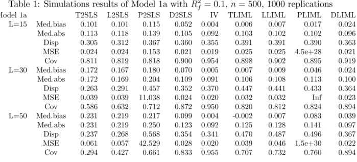
(21) Model 1a. l=(L + 1))4 ,l = 1; 2; :::; L where d is chosen so that l = d(1 2 Rf 0 = : 1 Rf2 Here, the instruments are ordered in decreasing order of importance. This model represents a case where there is some prior information about what instruments are important. Model 1b.. l. v u u Rf2 =t , l = 1; 2; :::; L: Here, there is no reason to prefer an 1 Rf2. instrument over another instrument as all the instruments have the same weight. Model 2 (Factor model). Wi = fi1 + fi2 + fi3 + ui where fi = (fi1 ; fi2 ; fi3 )0. iidN (0; I3 ), xi is a L. 1 vector of instruments constructed. from fi through xi = M fi + where. i. N (0;. 2. I3 ) with. i. = 0:3; and M is a L. 3 matrix which elements are. independently drawn in a U[-1, 1]. We report summary statistics for each of the following estimators: Carrasco’s (2012) regularized two-stage least squares, T2SLS (Tikhonov), L2SLS (Landweber Fridman), P2SLS (Principal component), Donald and Newey’s (2001) 2SLS (D2SLS), the unfeasible instrumental variable regression (IV), regularized LIML, TLIML (Tikhonov), LLIML (Landweber Fridman), PLIML (Principal component), and …nally Donald and Newey’s (2001) LIML (DLIML). For each of these estimators, the optimal regularization parameter is selected using Mallows Cp . We report the median bias (Med.bias), the median of the absolute deviations of the estimator from the true value (Med.abs), the di¤erence between the 0.1 and 0.9 quantiles (dis) of the distribution of each estimator, the mean square error (MSE) and the coverage rate (Cov.) of a nominal 95% con…dence interval. To construct the con…dence intervals to compute the coverage probabilities, we used the following estimate of asymptotic variance: (y V^ (^) =. W ^)0 (y n. W ^) ^ 0 (W. 19. 1. ^ 0W ^ (W 0 W ^) W. 1.

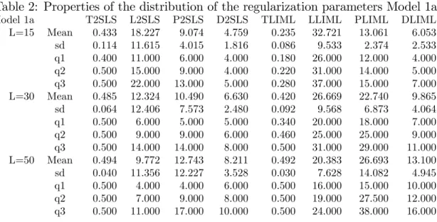
(22) ^ = P W. where W Tables 2, 4, and 6 contain summary statistics for the value of the regularization parameter which minimizes the approximate MSE. This regularization parameter is the number of instruments in DN,. for T, the number of iterations for LF, and the number. of principal components for PC3 . We report the mean, standard error (std), mode, …rst, second and third quartile of the distribution of the regularization parameter. Results on Models 1a and 1b are summarized in Tables 1, 2, 3, and 4. We …rst start by Model 1a where we can notice that the regularized LIML is better than the regularized 2SLS in almost every case. This dominance becomes clearer when the number of instruments increases. We observe that the coverage of regularized 2SLS is very poor while that for regularized LIML is much better, even though it is quite below 95%. Within the regularized LIML, T is the best especially when the number of instruments is very high, except in terms of coverage. However the DLIML is better than all the regularized LIML except for the coverage rate where PLIML is the best and for the median bias where TLIML and LLIML are better. But PLIML have very large MSE, median bias and dispersion. Overall, the performance of TLIML and LLIML is at par with DLIML even though in Model 1a, the instruments are ordered in decreasing order of importance which puts DN at an advantage. In Model 1b when all instruments have the same weights and there is no reason to prefer one over another, the regularized LIML strongly dominates the regularized 2SLS. The LF and T LIML dominate the DN LIML with respect to all the criteria. We can then conclude that in presence of many instruments and in absence of a reliable information on the relative importance of the instruments, the regularized LIML approach should be preferred to DN approach. We can also notice that when the number of instruments increases the MSE of regularized LIML becames smaller than those of regularized 2SLS. We observe that the MSE of DLIML explodes while those of TLIML and LLIML are stable, which can be explained by the existence of the moments of the regularized LIML, except for the PLIML which MSE also explodes. 3. The optimal for Tikhonov is searched over the interval [0.1,0.5] with 0.01 increment for Models 1a and 1b and the set {0, 0.000000001, 0.00000001, 0.0000001, 0.0000001, 0.000001, 0.00001, 0.01, 0.1, 0.2} for Model 2. The range of values for the number of iterations for LF is from 1 to 10 times the number of instruments and for the number of principal components is from 1 to the number of instruments.. 20.

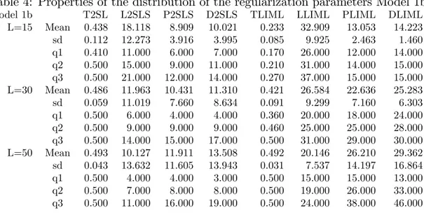
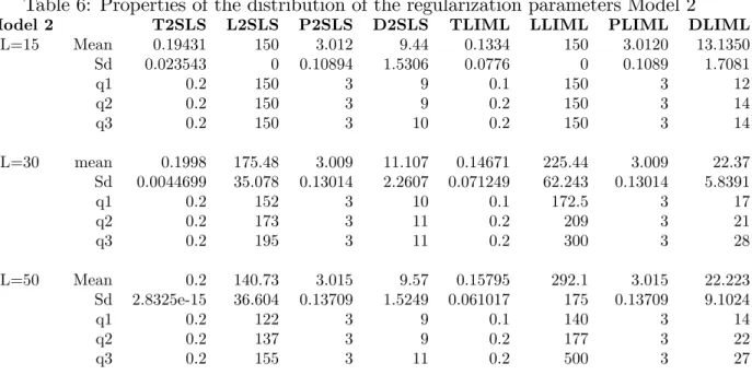
(23) Table 1: Simulations results of Model 1a with Rf2 = 0:1, n = 500, 1000 replications Model 1a L=15. L=30. L=50. Med.bias Med.abs Disp MSE Cov Med.bias Med.abs Disp MSE Cov Med.bias Med.abs Disp MSE Cov. T2SLS 0.101 0.113 0.305 0.024 0.811 0.172 0.172 0.263 0.039 0.586 0.231 0.231 0.237 0.061 0.294. L2SLS 0.101 0.118 0.312 0.024 0.819 0.167 0.169 0.291 0.039 0.632 0.219 0.219 0.268 0.057 0.427. P2SLS 0.115 0.139 0.367 0.153 0.818 0.180 0.204 0.457 11.038 0.712 0.217 0.250 0.568 42.529 0.661. D2SLS 0.052 0.105 0.360 0.021 0.900 0.070 0.109 0.352 0.024 0.872 0.099 0.123 0.354 0.028 0.833. IV 0.004 0.092 0.355 0.019 0.954 0.005 0.091 0.370 0.020 0.950 0.004 0.092 0.341 0.020 0.955. TLIML 0.006 0.103 0.391 0.025 0.898 0.007 0.106 0.447 0.032 0.820 -0.002 0.125 0.470 0.039 0.707. LLIML 0.007 0.102 0.391 0.025 0.902 0.009 0.108 0.441 0.032 0.812 0.007 0.128 0.487 0.046 0.732. PLIML 0.017 0.102 0.390 4.5e+28 0.895 0.046 0.113 0.433 Inf 0.824 0.083 0.141 0.496 1.5e+30 0.760. The poor performance of PC 2SLS and LIML in Models 1a and 1b can be explained by the absence of factor structure. Indeed, all eigenvalues of K (in the population) are equal to each other and consequently the Mallows Cp tend to select a large number of principal components (see Tables 2 and 4). The PC LIML is therefore close to the standard LIML estimator which is known for not having any moments. Now, we turn to Model 2 which is a factor model. From Table 5, we see that LIML dominates the 2SLS for all regularization schemes. But, there is no clear dominance among the regularized LIML as they all perform very well. The DLIML is dominated by regularized LIML for all measures. From Table 6, we can observe that PC selects three principal components in average corresponding to the three factors. We conclude this section by summarizing the Monte Carlo results. LLIML and TLIML are highly recommended if we are concerned with bias and mean square error. Selection methods as DN are recommended when the rank ordering of the strength of the instruments is clear. Otherwise, regularized methods are preferrable. Among the three regularizations, LF and T are more reliable than PC in absence of factor structure. Moreover, we observe small mean square errors for T and LF regularized LIML estimators which suggests the existence of moments.. 21. DLIML 0.024 0.096 0.363 0.021 0.919 0.024 0.100 0.364 0.023 0.894 0.039 0.097 0.367 0.022 0.894.

(24) Table 2: Properties of the distribution of the regularization parameters Model 1a Model 1a L=15. L=30. L=50. Mean sd q1 q2 q3 Mean sd q1 q2 q3 Mean sd q1 q2 q3. T2SLS 0.433 0.114 0.400 0.500 0.500 0.485 0.064 0.500 0.500 0.500 0.494 0.040 0.500 0.500 0.500. L2SLS 18.227 11.615 11.000 15.000 22.000 12.324 12.406 6.000 9.000 14.000 9.772 11.356 4.000 7.000 11.000. P2SLS 9.074 4.015 6.000 9.000 13.000 10.490 7.573 5.000 9.000 14.000 12.743 12.227 4.000 9.000 17.000. D2SLS 4.759 1.816 4.000 4.000 5.000 6.630 2.480 5.000 6.000 8.000 8.211 3.528 6.000 8.000 10.000. TLIML 0.235 0.086 0.180 0.220 0.280 0.420 0.092 0.340 0.460 0.500 0.492 0.030 0.500 0.500 0.500. LLIML 32.721 9.533 26.000 31.000 37.000 26.669 9.568 20.000 25.000 31.000 20.383 7.628 16.000 19.000 24.000. PLIML 13.061 2.374 12.000 14.000 15.000 22.740 6.873 18.000 25.000 29.000 26.693 14.082 15.000 27.500 38.000. DLIML 6.053 2.533 4.000 5.000 7.000 9.865 4.064 7.000 9.000 11.000 13.100 4.945 10.000 12.000 16.000. Table 3: Simulations results of Model 1 b with Rf2 = 0:1, n = 500, 1000 replications Model 1b L=15. L=30. L=50. Med.bias Med.abs Disp MSE Cov Med.bias Med.abs Disp MSE Cov Med.bias Med.abs Disp MSE Cov. T2SL 0.099 0.109 0.290 0.023 0.840 0.172 0.173 0.264 0.039 0.594 0.237 0.237 0.235 0.061 0.300. L2LS 0.096 0.115 0.297 0.023 0.843 0.165 0.165 0.277 0.038 0.643 0.226 0.226 0.259 0.058 0.406. P2LS 0.112 0.141 0.372 0.059 0.837 0.174 0.202 0.453 3.682 0.725 0.214 0.252 0.581 1.794 0.688. D2LS 0.128 0.146 0.346 0.042 0.805 0.219 0.237 0.457 907.310 0.673 0.257 0.285 0.590 4.946 0.639. 22. IV -0.006 0.087 0.347 0.019 0.946 0.006 0.091 0.355 0.020 0.952 -0.004 0.089 0.353 0.020 0.951. TLIML -0.000 0.103 0.390 0.024 0.897 0.010 0.107 0.412 0.030 0.829 -0.004 0.124 0.470 0.039 0.723. LLIML -0.001 0.102 0.386 0.025 0.899 0.011 0.110 0.421 0.033 0.828 0.000 0.126 0.489 0.045 0.723. PLIML 0.015 0.103 0.380 1.4e+28 0.891 0.042 0.111 0.413 1.3e+29 0.806 0.082 0.137 0.483 4.4e+30 0.752. DLIML 0.011 0.101 0.380 0.023 0.895 0.052 0.115 0.411 1.7e+30 0.801 0.107 0.156 0.526 3.8e+30 0.714.

(25) Table 4: Properties of the distribution of the regularization parameters Model 1b Model 1b L=15. L=30. L=50. Mean sd q1 q2 q3 Mean sd q1 q2 q3 Mean sd q1 q2 q3. T2SL 0.438 0.112 0.410 0.500 0.500 0.486 0.059 0.500 0.500 0.500 0.493 0.043 0.500 0.500 0.500. L2SLS 18.118 12.273 11.000 15.000 21.000 11.963 11.019 6.000 9.000 14.000 10.127 13.632 4.000 7.000 11.000. P2SLS 8.909 3.916 6.000 9.000 12.000 10.431 7.660 4.000 9.000 15.000 11.911 11.605 4.000 8.000 16.000. D2SLS 10.021 3.995 7.000 11.000 14.000 11.310 8.634 4.000 9.000 17.000 13.508 13.943 3.000 8.000 19.000. TLIML 0.233 0.085 0.170 0.210 0.270 0.421 0.091 0.360 0.460 0.500 0.492 0.031 0.500 0.500 0.500. LLIML 32.909 9.925 26.000 31.000 37.000 26.584 9.299 20.000 25.000 31.000 20.146 7.537 15.000 19.000 24.000. PLIML 13.053 2.463 12.000 14.000 15.000 22.636 7.160 18.000 25.000 29.000 26.210 14.197 15.000 26.000 38.000. DLIML 14.223 1.460 14.000 15.000 15.000 25.283 6.303 24.000 28.000 30.000 29.362 16.864 13.000 33.000 46.000. Table 5: Simulations results of Model 2 , n = 500, 1000 replications Model 2 L=15. Med.bias Med.abs Disp MSE cov. T2SLS 0.00033 0.017 0.066 0.00069 0.947. L2SLS 0.00014 0.0174 0.066 0.00069 0.946. P2SLS 0.00033 0.0176 0.066 0.00069 0.947. D2SLS 0.0039 0.0177 0.0658 0.00070 0.942. IV 0.00067 0.0179 0.0670 0.00068 0.952. TLIML -0.00033 0.0177 0.067 0.00069 0.948. LLIML -0.00023 0.0177 0.067 0.00069 0.948. PLIML -0.00025 0.017 0.067 0.00069 0.948. DLIML 0.00047 0.017 0.068 0.00070 0.946. L=30. Med.bias Med.abs Disp MSE cov. 0.0019 0.016 0.0668 0.00066 0.956. 0.0016 0.0170 0.0671 0.00066 0.955. 0.0016 0.0171 0.0672 0.00066 0.955. 0.0051 0.0174 0.0676 0.00069 0.949. 0.0013 0.0171 0.0668 0.00065 0.958. 0.0011 0.0171 0.0679 0.00066 0.953. 0.00095 0.0172 0.0677 0.00066 0.955. 0.00095 0.0172 0.0677 0.00066 0.955. 0.00193 0.0172 0.0685 0.00068 0.946. L=50. Med.bias Med.abs Disp MSE cov. 0.0010 0.0168 0.065 0.00065 0.945. 0.00036 0.0165 0.0656 0.00066 0.946. 0.000458 0.0165 0.0655 0.00066 0.947. 0.00352 0.0175 0.0666 0.00068 0.946. 0.00062 0.0171 0.0648 0.00065 0.95. 4.7045e-5 0.0167 0.0656 0.00066 0.945. -0.00034 0.0167 0.0654 0.00066 0.944. -0.00017 0.0167 0.065 0.00066 0.945. 0.00108 0.0177 0.067 0.00067 0.944. 23.

(26) Table 6: Properties of the distribution of the regularization parameters Model 2 Model 2 L=15. Mean Sd q1 q2 q3. T2SLS 0.19431 0.023543 0.2 0.2 0.2. L2SLS 150 0 150 150 150. P2SLS 3.012 0.10894 3 3 3. D2SLS 9.44 1.5306 9 9 10. TLIML 0.1334 0.0776 0.1 0.2 0.2. LLIML 150 0 150 150 150. PLIML 3.0120 0.1089 3 3 3. DLIML 13.1350 1.7081 12 14 14. L=30. mean Sd q1 q2 q3. 0.1998 0.0044699 0.2 0.2 0.2. 175.48 35.078 152 173 195. 3.009 0.13014 3 3 3. 11.107 2.2607 10 11 11. 0.14671 0.071249 0.1 0.2 0.2. 225.44 62.243 172.5 209 300. 3.009 0.13014 3 3 3. 22.37 5.8391 17 21 28. L=50. Mean Sd q1 q2 q3. 0.2 2.8325e-15 0.2 0.2 0.2. 140.73 36.604 122 137 155. 3.015 0.13709 3 3 3. 9.57 1.5249 9 9 11. 0.15795 0.061017 0.1 0.2 0.2. 292.1 175 140 177 500. 3.015 0.13709 3 3 3. 22.223 9.1024 14 22 27. 6 6.1. Empirical applications Returns to Schooling. A motivating empirical example is provided by the in‡uential paper of Angrist and Krueger (1991). This study has become a benchmark for testing methodologies concerning IV estimation in the presence of many (possibly weak) instrumental variables. The sample drawn from the 1980 U.S. Census consists of 329,509 men born between 1930-1939. Angrist and Krueger (1991) estimate an equation where the dependent variable is the log of the weekly wage, and the explanatory variable of interest is the number of years of schooling. It is obvious that OLS estimate might be biased because of the endogeneity of education. Angrist and Krueger (1991) propose to use the quarters of birth as instruments. Because of the compulsory age of schooling, the quarter of birth is correlated with the number of years of education, while being exogenous. The relative performance of LIML on 2SLS, in presence of many instruments, has been well documented in the literature (DN, Anderson, Kunitomo, and Matsushita (2010), and Hansen, Hausman, and Newey (2008)). We are going to compute the regularized version of LIML and compare it to the regularized 2SLS in order to show the empirical. 24.

(27) relevance of our method. We use the model of Angrist and Krueger (1991): logw =. + education +. 0 1Y. +. 0 2S. +". where logw = log of weekly wage, education = year of education, Y = year of birth dummy (9), S = state of birth dummy (50). The vector of instruments Z = (1; Y; S; Q; Q. OLS 0.0683 (0.0003). Y; Q. S) includes 240 variables. Table 7 reports schooling coe¢ cients. Table 7: Estimates of the return to education. 2SLS 0.0816 (0.0106) LIML 0.0918 (0.0101). T2SLS 0.1237 (0.0482) = 0.00001 TLIML 0.1237 (0.0480) = 0.00001. L2SLS 0.1295 (0.0272) Nb of iterations 700 LLIML 0.1350 (0.0275) Nb of iterations 700. P2SLS 0.1000 (0.0411) Nb of eigenfunctions 81 PLIML 0.107 (0.0184) Nb of eigenfunctions 239. generated by di¤erent estimators applied to the Angrist and Krueger data along with their standard errors in parentheses. Table 7 shows that all regularized 2SLS and LIML estimators based on the same type of regularization give close results. The coe¢ cients we obtain by regularized LIML are slightly larger than those obtained by regularized 2SLS suggesting that these methods provide an extra bias correction, as observed in our Monte Carlo simulations. Note that the bias reduction obtained by regularized LIML compared to standard LIML comes at the cost of a larger standard error. Among the regularizations, PC gives estimators which are quite a bit smaller than T and LF. However, we are suspicious of PC because there is no factor structure here.. 6.2. Elasticity of Intertemporal Substitution. In macroeconomics and …nance, the elasticity of intertemporal substitution (EIS) in consumption is a parameter of central importance. It has important implications for the relative magnitudes of income and substitution e¤ects in the intertemporal consumption decision of an investor facing time varying expected returns. Campbell and Viceira (1999) show that when the EIS is less (greater) than 1, the investor’s optimal consumption-wealth ratio is increasing (decreasing) in expected returns.. 25.

(28) Yogo (2004) analyzes the problem of EIS using the linearized Euler equation. He explains how weak instruments have been the source for an empirical puzzle namely that using conventional IV methods the estimated EIS is signi…cantly less than 1 but its reciprocal is not di¤erent from 1. In this subsection, we follow one of the speci…cations in Yogo (2004) using quarterly data from 1947.3 to 1998.4 for the United States and compare all the estimators considered in the present paper. The estimated models are given by the following equation: ct+1 =. + rf;t+1 +. t+1. and the "reverse regression": rf;t+1 = where. is the EIS,. +. 1. ct+1 +. t+1. ct+1 is the consumption growth at time t + 1, rf;t+1 is the real. return on a risk free asset,. and. are constants, and. t+1. and. t+1. are the innovations. to consumption growth and asset return, respectively. To solve the empirical puzzle, we increase the number of instruments from 4 to 18 by including interactions and power functions. The four instruments used by Yogo (2004) are the twice lagged, nominal interest rate (r), in‡ation (i), consumption growth (c) and log dividend-price ratio (p). The set of instruments is then Z = [r; i; c; p]. The 18 instruments used in our regression are derived from Z and are given by4 II = [Z; Z:2 ; Z:3 ; Z(:; 1) Z(:; 2); Z(:; 1) Z(:; 3); Z(:; 1) Z(:; 4); Z(:; 2) Z(:; 3); Z(:; 2) Z(: ; 4); Z(:; 3) Z(:; 4)]. Since the increase of the number of instruments improves e¢ ciency and regularized 2SLS and LIML correct the bias due to the use of many instruments, the increase of the number of instruments will certainly enable us to have better points estimates. Interestingly, the point estimates obtained by LF and T regularized estimators are close to those used for macro calibrations (EIS equal to 0.71 in our estimations and 0.67 in Castro, Clementi, and Macdonald (2009)). For LF estimator, 2SLS and LIML 4. k Z:k = [Zij ] , Z(:; k) is the k th column of Z and Z(:; k) Z(:; l) is a vector of interactions between columns k and l.. 26.

(29) regularizations give very close estimators. Moreover, the results of the two equations are consistent with each other since we obtain the same value for. in both equations. PC seems to take too many factors, and. did not perform well, this is possibly due to the fact that there is no factor structure.. 2SLS (18 instr) 0.1884 (0.0748). 0.6833 (0.4825). 0.8241 (0.263). LIML (4 instr) 0.0293 (0.0994). LIML (18 instr) 0.2225 ( 0.0751). 34.1128 (112.7122). 4.4952 (0.5044). 1=. 1=. 7. Table 8: Estimates of the EIS. 2SLS (4 instr) 0.0597 (0.0876). T2SLS 0.71041 (0.093692) = 0.0001 1.406 (0.2496) = 0.01 TLIML 0.71041 (0.093692) = 0.01 1.407 (0.249) = 0.01. Nb of. Nb of. Nb of. Nb of. L2SLS 0.71063 ( 0.093689) iterations 300 1.407 (0.249) iterations 300 LLIML 0.71063 ( 0.093689) iterations 300 1.4072 (0.249) iterations 300. P2SLS 0.1696 (0.077808) Nb of PC 11 0.7890 (0.246) Nb of PC 17 PLIML 0.1509 (0.077835) Nb of PC 8 3.8478 (0.37983) Nb of PC 17. Conclusion. In this paper, we propose a new estimator which is a regularized version of LIML estimator. Our framework has the originality to allow for a …nite and in…nite number of moment conditions. We show theoretically that regularized LIML improves upon regularized 2SLS in terms of smaller leading terms of the MSE. All the regularization methods involve a tuning parameter which needs to be selected. We propose a datadriven method for selecting this parameter and show that this selection procedure is optimal. Moreover, we prove that the LIML estimator based on principal components has …nite moments. Although, we were not able to prove this result for LIML regularized with T and LF, the simulations suggest that their …rst two moments exist. Our simulations show that the leading regularized estimators (LF and T of LIML) are nearly median unbiased and dominate regularized 2SLS and standard LIML in terms of MSE. We restrict our work in this paper to the estimation and asymptotic properties of regularized LIML with many strong instruments. One possible topic for future research. 27.

(30) would be to extend these results to the case of weak instruments as in Hansen, Hausman, and Newey (2008). Moreover, it would be interesting to study the behavior of other k-class estimators, such as Fuller’s (1977) estimator and bias corrected 2SLS estimator, in presence of many (and possibly weak) instruments. Another interesting topic is the use of our regularized LIML or 2SLS for inference when facing many instruments or a continuum of instruments. This would enable us to compare our inference with those of Hansen, Hausman, and Newey (2008) and Newey and Windmeijer (2009).. 28.

(31) References Andersen, T. G., and B. E. Sorensen (1996): “GMM Estimation of a Stochastic Volatility Model: A Monte Carlo Study,”Journal of Business & Economic Statistics, 14(3), 328–52. Anderson, T. (2010): “The LIML estimator has …nite moments!,”Journal of Econometrics, 157(2), 359–361. Anderson, T., N. Kunitomo, and Y. Matsushita (2010): “On the asymptotic optimality of the LIML estimator with possibly many instruments,”Journal of Econometrics, 157(2), 191–204. Angrist, J. D., and A. B. Krueger (1991): “Does Compulsory School Attendance A¤ect Schooling and Earnings?,”The Quarterly Journal of Economics, 106(4), 979– 1014. Bai, J., and S. Ng (2010): “Instrumental Variable Estimation in a Data Rich Environment,” Econometric Theory, 26, 1577–1606. Bekker, P. A. (1994): “Alternative Approximations to the Distributions of Instrumental Variable Estimators,” Econometrica, 62(3), 657–81. Belloni, A., D. Chen, V. Chernozhukov, and C. Hansen (2012): “Sparse models and Methods for Optimal Instruments with an Application to Eminent Domain,” Econometrica, 80, 2369–2429. Campbell, J. Y., and L. M. Viceira (1999): “Consumption And Portfolio Decisions When Expected Returns Are Time Varying,” The Quarterly Journal of Economics, 114(2), 433–495. Carrasco, M. (2012): “A regularization approach to the many instruments problem,” Journal of Econometrics, 170(2), 383–398. Carrasco, M., and J.-P. Florens (2000): “Generalization Of GMM To A Continuum Of Moment Conditions,” Econometric Theory, 16(06), 797–834.. 29.

(32) (2012): “On the Asymptotic E¢ ciency of GMM,”forthcoming in Econometric Theory. Carrasco, M., J.-P. Florens, and E. Renault (2007): “Linear Inverse Problems in Structural Econometrics Estimation Based on Spectral Decomposition and Regularization,”in Handbook of Econometrics, ed. by J. Heckman, and E. Leamer, vol. 6, chap. 77. Elsevier. Castro, R., G. L. Clementi, and G. Macdonald (2009): “Legal Institutions, Sectoral Heterogeneity, and Economic Development,” Review of Economic Studies, 76(2), 529–561. Chao, J. C., and N. R. Swanson (2005): “Consistent Estimation with a Large Number of Weak Instruments,” Econometrica, 73(5), 1673–1692. Craven, P., and G. Wahba (1979): “Smoothing noisy data with spline functions: Estimating the correct degree of smoothing by the method of the generalized crossvalidation,” Numer. Math., 31, 377–403. Dagenais, M. G., and D. L. Dagenais (1997): “Higher moment estimators for linear regression models with errors in the variables,”Journal of Econometrics, 76(12), 193–221. Donald, S. G., and W. K. Newey (2001): “Choosing the Number of Instruments,” Econometrica, 69(5), 1161–91. Fuller, W. A. (1977): “Some Properties of a Modi…cation of the Limited Information Estimator,” Econometrica, 45(4), 939–953. Guggenberger, P. (2008): “Finite Sample Evidence Suggesting a Heavy Tail Problem of the Generalized Empirical Likelihood Estimator,”Econometric Reviews, 27(46), 526–541. Hahn, J., and J. Hausman (2003): “Weak Instruments: Diagnosis and Cures in Empirical Econometrics,” American Economic Review, 93(2), 118–125.. 30.

(33) Hahn, J., and A. Inoue (2002): “A Monte Carlo Comparison Of Various Asymptotic Approximations To The Distribution Of Instrumental Variables Estimators,” Econometric Reviews, 21(3), 309–336. Hansen, C., J. Hausman, and W. Newey (2008): “Estimation With Many Instrumental Variables,” Journal of Business & Economic Statistics, 26, 398–422. Hansen, C., and D. Kozbur (2013): “Instrumental Variables Estimation with Many Weak Instruments Using Regularized JIVE,” mimeo. Hausman, J., R. Lewis, K. Menzel, and W. Newey (2011): “Properties of the CUE estimator and a modi…cation with moments,”Journal of Econometrics, 165(1), 45 –57. Hausman, J. A., W. K. Newey, T. Woutersen, J. C. Chao, and N. R. Swanson (2012): “Instrumental variable estimation with heteroskedasticity and many instruments,” Quantitative Economics, 3(2), 211–255. James, A. (1954): “Normal Multivariate Analysis and the Orthogonal Group,”Annals of Mathematical Statistics, 25, 46–75. Kapetanios, G., and M. Marcellino (2010): “Factor-GMM estimation with large sets of possibly weak instruments,”Computational Statistics and Data Analysis, 54, 2655–2675. Kleibergen, F. (2002): “Pivotal Statistics for Testing Structural Parameters in Instrumental Variables Regression,” Econometrica, 70(5), 1781–1803. Kress, R. (1999): in Linear Integral Equationsvol. 82, p. 388. Springer, 2 edn. Kuersteiner, G. (2012): “Kernel-weighted GMM estimators for linear time series models,” Journal of Econometrics, 170, 399–421. Li, K.-C. (1986): “Asymptotic optimality of CL and generalized cross-validation in ridge regression with application to spline smoothing,”The Annals of Statistics, 14, 1101–1112.. 31.

(34) (1987): “Asymptotic optimality for Cp , CL , cross-validation and generalized cross-validation: Discrete Index Set,” The Annals of Statistics, 15, 958–975. Mallows, C. L. (1973): “Some Comments on Cp,” Technometrics, 15, 661–675. Nagar, A. L. (1959): “The bias and moment matrix of the general k-class estimators of the parameters in simultaneous equations,” Econometrica, 27(4), 575–595. Newey, W. K., and F. Windmeijer (2009): “Generalized Method of Moments With Many Weak Moment Conditions,” Econometrica, 77(3), 687–719. Okui, R. (2011): “Instrumental variable estimation in the presence of many moment conditions,” Journal of Econometrics, 165(1), 70 –86. Stone, C. J. (1974): “Cross-validatory choice and assessment of statistical predictions,” Journal of the Royal Statistical Society, 36, 111–147. Yogo, M. (2004): “Estimating the Elasticity of Intertemporal Substitution When Instruments Are Weak,” The Review of Economics and Statistics, 86(3), 797–810.. 32.

(35) A. Proofs. Proof of Proposition 1 We want to prove that the regularized LIML estimators have …nite moments. These estimators are de…ned as follow 5 : ^ = (W 0 (P. 1. In ) W ). W 0 (P. In ) y. (y W )0 P (y W ) and P = T (Kn ) (y W )0 (y W ) ^ = W 0 (P ^ = W 0 (P Let us de…ne H In ) W and N where. = min. ^=H ^. 1. X. X. ED E D ) y; ^ j W l ; ^ j :. (qj. j. By the Cauchy-Schwarz inequality and because j ^ vl j jH. p matrix with a typical element. 1 vector with a typical element Nl =. l. In ) y thus. D ED E ) W v ; ^ j W l; ^ j. (qj. j. ^ is a p and N. T .. ^: N. ^ is a p If we denote W v = (W1v ; W2v ; :::; Wnv )0 , H ^ vl = H. 1. v. 2kW kkW k and jNl j. l. j. 1; jqj j. 1; we can prove that. 2kykkW k:. Under our assumptions, all the moments (conditional on X) of W and y are …nite, we ^ and N ^ have …nite moments. can conclude that all elements of H The ith element of ^ is given by: ^i =. p X j=1. ^ jHj. 1. ^ ij )Nj cof (H. ^ ij ) is the signed cofactor of H ^ ij , Nj is the j th element of N ^ and j : j denotes where cof (H 5. Let g and h be two p vectors of functions of L2 ( ). By a slight abuse of notation, g; h0 denotes the matrix with elements ga ; hb ; a; b = 1; :::; p. 33.

(36) the determinant. j ^i jr Let. 1. >. 2. ^ jHj. r. j. p X j=1. ^ ij )Nj jr cof (H. be two regularization parameters. It turns out that P. de…nite negative and hence 0. 2. 1. P. 1. . This will be used in the proof.. 2. is semi. 6. We also have that (y W )0 P (y W ) (y W )0 (y W ) c0 c max 0 = max qj : c j cc. = min. ^ We want to prove that jHj. jSj where S is a positive de…nite p. p matrix to be. speci…ed later on. We want to show that P. 2. In is positive de…nite. Let us consider x 2 Rn . We. have x0 P. In x = 2. X. (qj. 2. ) x;. j. 0. x;. j. j. =. X. (qj. 2. j. =. X. j;qj >. +. X. j;qj. ) k x;. (qj. j. k2. 2. ) k x;. j. k2. 2. ) k x;. j. k2 : (2). (1). 2. (qj 2. We know that qj is a decreasing sequence. Hence there exists j such that qj j < j and qj <. 2. 2. for. for j > j and. x0 P. In x = 2. X. (qj. 2. ) k x;. j. k2. 2. ) k x;. j. k2 : (2). j j. +. X. (qj. j>j. (1). The term (1) is positive and the term (2) is negative. As n increases, 6. Note that if the number of instruments is smaller than n we can compare by P , the projection matrix on the instruments, and . It turns out that P …xed and hence 0 as in Fuller (1977).. 34. decreases and. obtained with P replaced P is de…nite negative for.

(37) qj increases for all j while. 2. also increases. Note that in the case of SC, qj switches. from 1 to 0 at j so that the variation in. of qj at j = j is greater than the variation. of. decreases. We were not able to prove this. 2. : It follows that j increases when. result in the case of T and LF. The term (2) goes to zero as n goes to in…nity. Indeed when j goes to in…nity, we have X. j>j. (qj. ) k x; 2. k2. j. ;. X. j>j. k x;. We can conclude that for n su¢ ciently large,. j. k2 = op (1):. is small and j is su¢ ciently large. for (2) to be smaller in absolute value than (1) and hence x0 Denote S = (. 2. P. 2. In x > 0.. )W 0 W we have ^ = W 0 (P H. In ) W. = W0 P. 2. = W0 P. 2. In W + (. 2. )W 0 W. In W + S:. Hence, ^ = jW 0 P jHj. 2. = jSjjIp + S. 1=2. In W + Sj W0 P. 2. In W S. 1=2. j. jSj: For n large but not in…nite,. 2. > 0 and jSj > 0. As in Fuller (1977) using James. (1954), we can show that the expectation of the inverse 2rth power of the determinant of. S exists and is bounded for n greater than some number n(r), since S is expressible as a product of multivariate normal r.v.. Thus we can apply Lemma B of Fuller (1977) and conclude that the regularized LIML has …nite rth moments for n su¢ ciently large but …nite. At the limit when n is in…nite, the moments exist by the asymptotic normality of the estimators established in Proposition 2. Proof of Proposition 2 To prove this proposition we …rst need the following lemma.. 35.

(38) Lemma 1 (Lemma A.4 of DN) P P ^ ! If A^ ! A and B B. A is positive semi de…nite and B is positive de…nite, 0A argmin 1 =1 0 exists and is unique (with = ( 1 ; 02 )0 and 1 2 R) then B. ^ = argmin Let H = E(fi fi0 ) , P. 1 =1. 0A ^ 0B ^. !. 0. =. 0. is a symmetric idempotent matrix for SC and PC matrix. but not necessarily for T and LF. We want to show that ^ !. as n and n. 1 2. go to in…nity.. We know that 0 ^ = argmin (y W ) P (y W ) (y W )0 (y W ) 0 0 b (1; 0 )A(1; ) = argmin 0 0 b (1; 0 )B(1; ). 0 ^ = W W and W = [y; W ] = W D0 + "e, where D0 = [ 0 ; I], where A^ = W 0 P W =n, B n 0 is the true value of the parameter and e is the …rst unit vector.. In fact A^ = W 0 P W =n D00 W 0 P W D0 D00 W 0 P "e e0 "0 P W D0 e0 "0 P "e = + + + : n n n n n. 1X Let us de…ne gn = Z(:; xi )Wi , g = EZ(:; xi )Wi and g; g 0 n. K. is a p. p matrix with. i=1. (a, b) element equal to K. 1 2. 1 2. E(Z(:; xi )Wia ); K. E(Z(:; xi )Wib ) where Wia is the ath. element of Wi vector. D00 W 0 W D0 n. D00 (Kn ). =. D00 HD0 + op (1). ! D00 g; g 0 as n and n. 1 2. go to in…nity and. 1 2. =. K. gn ; (Kn ). 1 2. gn0 D0. D0. ! 0, see the proof of Proposition 1 of Carrasco. 36.

(39) (2012). We also have by Lemma 3 of Carrasco (2012): n 1 1X 1 "e = D00 (Kn ) 2 gn ; (Kn ) 2 Z(:; xi )"i e = op (1), n n i=1 n 1 1X 1 e0 "0 W D0 = e0 (Kn ) 2 Z(:; xi )"i ; (Kn ) 2 gn0 D0 = op (1), n n i=1 n n 0 0 X 1 1 1 1X e " "e = e0 (Kn ) 2 Z(:; xi )"i ; (Kn ) 2 Z(:; xi )"0i e = op (1): n n n D00 W 0. i=1. i=1. We can then conclude that A^ ! A = D00 g; g 0. and. K. D0 as n and n. 1 2. go to in…nity. ! 0.. Note that H = g; g 0. because by assumption ga = E(Z(:; xi )fia ) belongs to the. K. range of K. Let L2 (Z) be the closure of the space spanned by fZ(x; );. 2 Ig and g1. be an element of this space. If fi 2 L2 (Z) we can compute the inner product and show that ga ; gb. K. = E(fia fib ) by applying Theorem 6.4 of Carrasco, Florens, and Renault. (2007). Thus A = D00 HD0 . ^ ! B = E(Wi W 0 ) B i by the law of large numbers with Wi = [yi Wi0 ]0 . The LIML estimator is given by b )A(1; 0 b )B(1; 0. ^ = argmin (1; (1;. 0 0 ) 0 0 ). ;. so that it su¢ ces to verify the hypotheses of Lemma 1. For. = (1;. 0. ) 0. A. =. 0. D00 HD0. = (. 0. )H(. = (. 0. )E(fi fi0 )(. Because H is positive de…nite, we have. 0. A. 37. 0. )0 0. )0. 0, with equality if and only if. =. 0..

(40) Also, for any 0. = ( 1;. B. 0 0 2). = E[( 1 yi + Wi0. 2 2) ]. = E[( 1 "i + (fi + ui )0 (. 1 0. = E[( 1 "i + u0i (. 2 2 )) ]. Then by H nonsingular 1. 6= 0 partitioned conformably with (1; 0 ), we have. 0. 6= 0 and hence. 0. 1 0. +. B > 0 for any. +. 2 2 )) ]. +(. with. 1 0. 1 0. 0 2 ) H( 1 0. +. +. 6= 0. If. 2. 2 2 1. B =. +. 1 0. 2). +. 2. = 0 then. > 0. Therefore B is positive de…nite. 0A It follows that = 0 is the unique minimum of 0 . B 1 p Now by Lemma 1 we can conclude that ^ ! 0 as n and n 2 go to in…nity.. Proof of asymptotic normality: Let A( ) = (y W )0 P (y W )=n , B( ) = (y W )0 (y W )=n and ( ) =. A( ) . B( ). We know that the LIML is ^ = argmin ( ): The gradient and Hessian are given by ( ) = B( ) ( ) = B( ). 1. [A ( ). 1. ( )B ( )]. [A ( ). ( )B ( )]. B( ). 1. [B ( ). 0. ( ). ( )B 0 ( )]. Then by a standard mean-value expansion of the …rst-order conditions. (^) = 0. with probability one. p. n(^. 0). 1. =. P where ~ is the mean-value. By Lemma 1, ~ !. p (~) n. ( 0). 0.. P It then follows, as in the proof of Lemma 1, that B(~) !. 0;. P (~) ! 0 where. u". P. 2 "; B P. P (~) !. 2. u" ;. p (~) !. = E(ui "i ) and B (~) = 2W 0 W=n ! 2E(Wi Wi0 ); A (~) =. 2W 0 P W=n ! 2H with H = E(fi fi0 ). P. So that ~ 2 (~)=2 ! H with ~ 2 = "0 "=n. 0 p p W" u" Let ^ = 0 , = 2 and v = u " 0 : We have v 0 P "= n = Op (1= n ) = op (1) "" " using Lemma 5(iii) of Carrasco (2012) and E (vi "i ) = 0. p ^ = Op (1= n) by the Central limit theorem and delta method. Also "0 P " = p Op (1= ) as in Carrasco (2012). So that ( ^ )"0 P "= n = Op (1=n ) = op (1). p Furthermore, f 0 (I P ) "= n = Op ( 2 ) = op (1) by Lemma 5(ii) of Carrasco. 38.

(41) p. P )2 f =n).. = tr(f 0 (I. (2012) with n~ 2. ( 0 )=2 = (W 0 P " = (f 0 ". W 0" p )= n "0 " P ) " + v0P ". "0 P ". f 0 (I. p d = f 0 "= n + op (1) ! N (0;. p )"0 P ")= n. (^. 2 " H):. The conclusion follows from Slutzky theorem. Proof of Proposition 3 To prove this proposition, we need some preliminary result. To simplify, we omit the hats on. j. and. j. and we denote P. and q( ;. j). by P and qj in the sequel.. Lemma 2: Let ~ = "0 P "=(n. 2 "). (^) with. and ^ =. ( ) =. (y W )0 P (y W ) . If the (y W )0 (y W ). assumptions of Proposition 2 are satis…ed, then ^. p where. ;n. ^ nR. ( ^2" =. =. ~. =. ~ + o(1=n );. = o(. 1) ~. 2 ". "0 f (f 0 f ). 1 0. f "=2n. 2 ". ^ +R. ;n );. = trace(S( )).. Proof of Lemma 2: It can be shown similarly to the calculations in Proposition 1 that. ( ) is three times continuously di¤erentiable with derivatives that are bounded. in probability uniformly in a neighborhood of p ( 0 ) + O(1= n). It implies that ^= Then expanding ^. 0. +[. (^) around. 0. =. ( 0). (^. =. ( ^0 ). ( 0 )]. 1. 0.. For any ~ between. 0. and ^;. ( 0 ) + O(1=n):. gives 0 0). ( 0 )0 [. ( 0 )(^ ( 0 )]. 1. 0 )=2. ( 0 )=2 + O(1=n3=2 ):. As in proof of Proposition 1 and in Lemma A.7 of DN. 39. + O(1=n3=2 ). (~) =.

(42) p. n^ 2". ( 0 )=2 = h + Op ( ^ 2". 1=2. +. p. 1=n ) with h = f 0 "=n. Moreover, 1=2. ( 0 )=2 = H + Op (. +. p 1=n ). And by combining these two equalities, we obtain ( 0 )0 [. 1. ( 0 )]. ( 0 ) = h0 H. 1. h=(n. 2 "). + O(. 1=2. =n +. p 1=(n3 )):. Note also that ( 0) = (. 2 2 ~ " =^ " ). ~. (^ 2" =. =. =~. (^ 2" =. 1) ~ + ~ (^ 2". 2 ". 2 2 2 2 " ) =(^ " " ). p 1) ~ + O( 1=n3 ). 2 ". = tr(S( )). n. = tr(. tr(P 2 1 [ v "H. 2). +. n 2) tr(P = tr( 2" H 1 [ v ]H n = O(1=n ) + :. We then have that. p p n 1=(n3 ) = o(. f 0 (I. P )2 f n. 1. ) + tr(. n). and. ]H. 1. ). 2 1 f [ "H. p. n. 1=2. 0 (I. P )2 f n. =n = o(. n ):. combining equations give ^=~. ( ^2" =. 1) ~. 2 ". "0 f (f 0 f ). 1 0. f "=2n. 2 ". ^ +R. and p. ^ = o( nR. ;n ):. By using ~ = O(1=n ), it is easy to prove that ^ = ~ + o(1=n ) . Lemma 3: If the assumptions of Proposition 3 are satis…ed, then ~. i) u0 P u. u. = o(1=n ),. X p ii) E(h ~ "0 v= njX) = (tr(P )=n) fi E("2i vi0 jxi )=n + O(1=(n2 )), 0. iii) E(hh H. 1. p. i. h= njX) = O(1=n).. 40. ]H. 1. ). Using this and.

(43) Proof of Lemma 3: For the proof of i), note that E( ~ =X) = tr(P E("0 "))=n. 2 ". =. tr(P )=n: Similarly, we have E(u0 P ujX) = tr(P ). u. and by Lemma 5 (iv) of Carrasco (2012). using " in place of u we have E[( ~. tr(P )=n)2 jX] = [. 4 2 " tr(P ). + o(tr(P )2 )]=(n2. 4 "). (tr(P )=n)2 = o((tr(P )=n)2 ):. Thus, ( ~. tr(P )=n) u = o(tr(P )=n) = o(1=n ) by Markov inequality. tr(P ) 0 ~ u = o(1=(n )). And u0 P u u = o(1=n ) such that u P u n To show ii) we can notice that p p E(h ~ "0 v= njX) = E(h"0 P ""0 v=(n 2" n)jX) X = E(fi "i "j Pjk "k "l vl02 2" )jX) i;j;k;l. =. X i. +. X i6=j. fi Pii E("4i vi0 jxi )=n2. 2 ". i6=j. fi Pjj E("2i vi jxi )=n2. = O(1=n) + (tr(P )=n). X + 2 fi Pij E("2j vj0 jxj )=n2. X i. fi E("2i vi0 jxi )=n. This is true because E("4i vi0 jxi ) and E("2i vi0 jxi ) are bounded by Assumption 2 hence f 0 P =n is bounded for. i. = E("4i vi0 jxi ) and. i. = E("2i vi0 jxi ).. For iii) E(hh0 H. 1. X p h= njX) = E(fi "i "j fj0 H. 1. i;j;k. =. X i. E("3i jxi )fi fi0 H. fk "k jX)=n2 1. fi =n2. = O(1=n): Now we turn to the proof of Proposition 3. Proof of Proposition 3 Our proof strategy will be very close to those of Carrasco (2012) and DN. To obtain. 41.

(44) the LIML, we solve the following …rst order condition W ^). W 0 P (y. ^ W 0 (y. W ^) = 0. with ^ = (^): Let us consider. p. n(^. ^ )=H. 1^. ^ = W 0 P W=n h with H. p ^ = W 0 P "= n h. ^ W 0 W=n and. p ^ W 0 "= n:. As in Carrasco (2012) we are going to apply Lemma A.1 of DN7 . 5 X p ^ h=h+ Tjh + Z h with h = f 0 "= n, j=1. p P )"= n = O( 1=2 ) p p p T2h = v 0 P "= n = O( 1=n ), T3h = ~ h0 = O(1=n ); T4h = ~ v 0 "= n = O(1=n ), p p T5h = h0 H 1 h u" =2 n 2" = O(1= n), p p 0 ^ W 0 "= n ( ^ ~ R ^ ) n(W 0 "=n ^ Zh = R u" ) where R is de…ned in Lemma 2. p 0 h By using the central limit theorem on n(W 0 "=n u" ) and Lemma 2, Z = O( n ). T1h =. f 0 (I. The results on order of Tjh hold by Lemma 5 Carrasco (2012). We also have 3 X ^ =H+ H TjH + Z H ; j=1. T1H. =. T3H =. 0. f (I. p ), T2H = (u0 f + f 0 u)=n = O(1= n);. P )f =n = O(. ~ H = O(1=n ); ~. Z H = u0 P u=n. u. ^ W 0 W=n + ~ (H +. By Lemma 3, u0 P u=n. u). u0 (I. P )f =n. f 0 (I. P )u=n:. ~. v = o(1=n ). Lemma 5 (ii) of Carrasco (2012) implies p u0 (I P )f =n = O( 1=2 = n) = o( n ). By the central limit theorem, W 0 W=n = p H + u + O(1= n).. ^ W 0 W=n. ~ (H +. u). = (^. ~ )W 0 W=n + ~ (W 0 W=n. H. p = o(1=n ) + O(1=n )O(1= n) = o( thus, Z H = o( 7. n. ).. The expression of T5h , Z h and Z H below correct some sign errors in DN. 42. u) n. ).

(45) We apply Lemma A.1 of DN with 5 3 X X h h H T = Tj , T = TjH , j=1. j=1. 5 5 5 5 X X X X h h 0 h h h 0 h h Z =( Tj )( Tj ) + ( Tj )(T1 + T2 ) + (T1 + T1 )( Tjh )0 ; A. j=3. j=3. j=3. j=3. and 5 5 X X 0 ^ ) = hh0 + A( hTjh + Tjh h0 +(T1h +T2h )(T1h +T2h )0 hh0 H j=1. Note that hT3h. 0. 1. j=1. hh0 H. 1. 3 X. TjH. 0. j=1. 3 X. TjH H. 1. hh0 :. j=1. 0. T3H = 0.. Also we have E(hh0 H. 1. (T1H +T2H )jX) =. 2 " ef (. 0. )+O(1=n), E(T1h h0 ) = E(hT1h ) =. 0. ), E(T1h T1h ) = 2" e2f ( ) where f 0 (I P )2 f f 0 (I P )f and e2f ( ) = . ef ( ) = n n tr(P ) X 1 0 By Lemma 3 (ii) E(hT4h jX) = : fi E("2i vi0 jxi )=n + O n n2 i By Lemma 5 (iv) of Carrasco (2012), with v in place of u and noting that 2 " ef (. v". = 0,. we have 0. E(T2h T2h jX) = 0. E(hT2h jX) =. X i. 2 ". v. tr(P 2 ) ; n. Pii fi E("2i vi0 jxi )=n:. 0. By Lemma 3 (iii), E(hT5h ) = O(1=n). X X tr(P ) X For ^ = Pii fi E("2i vi0 jxi )=n fi E("2i vi0 jxi )=n Pii (1 Pii )fi E("2i vi0 jxi )=n; n i i i ^ ) satis…es A( ^ )jX) = E(A(. 2 "H. +. 2 ". v. tr(P 2 ) + n. We can also show that kT1h kkTjh k = o(. kTkh kkTjH k = o(. n. n. 2 " e2f. 0. + ^ + ^ + O(1=n). ), kT2h kkTjH k = o(. n. ) for each j and k > 2. Furthermore kTjH k2 = o(. follows that Z A = o(. n. ) for each j and n. ) for each j. It. ). It can be noticed that all conditions of Lemma A.1 of DN. are satis…ed and the result follows by observing that E("2i vi0 jxi ) = 0. This ends the proof of Proposition 3.. 43.

(46) To prove the Proposition 4 we need to establish the following result. Lemma 4 (Lemma A.9 of DN): If sup (jS^ ( ) 2Mn. P. P. S ( )j=S ( )) ! 0, then. S (^ )= inf S ( ) ! 1 as n and n ! 1 2Mn. Proof of Lemma 4: We have that inf S ( ) = S ( the …niteness of the index set for 1=. 2Mn. ) for some. in Mn by. for PC, SC and LF and by the compactness of. the index set for T. Then, the proof of Lemma 4 follows from that of Lemma A.9 of DN.. Proof of Proposition 4 We proceed by verifying the assumption of Lemma 4. f 0 (I P )2 f tr(P 2 ) ^ m ( ), R ^ cv ( ); or Let R( ) = + 2u be the risk approximated by R n n " # 2 f 0 (I P )2 f 2 tr(P ) ^ lcv ( ), and S ( ) = 2 R + . For notational convenience, " v n n we henceforth drop the subscript on S and R. For Mallows Cp , generalized crossvalidation and leave one out cross-validation criteria, we have to prove that sup 2Mn. ^ ) jR(. R( )j=R( ) ! 0. (6). in probability as n and n ! 1: To establish this result, we need to verify the assumptions of Li’s (1987, 1986) theorems. We treat separately the regularizations with a discrete index set and that with a continuous index set (Tikhonov regularization). SC and LF have a discrete index set in terms of 1= . Discrete index set: We recall the assumptions of Li (1987) (A.1) to (A.3’) for m = 2. (A.1) lim sup. (P ) < 1 where (P ) is the largest eigenvalue of P ;. (A.2). 1;. n!1 2Mn E((ui e)8 ) <. (A.3’) inf nR( ) ! 1: 2Mn. (A.1) is satis…ed because for every. 2 Mn ; all eigenvalues fqj g of P are less than. or equal to 1. (A.2) holds by our assumption 4 (i). For (A.3’), note that nR( ) = f 0 (I. P )2 f +. 44. 2 u. tr(P 2 ) = Op n. +. 1. :.