Tax Evasion and Social Interactions

Texte intégral

(1)2004s-61. Tax Evasion and Social Interactions Bernard Fortin, Guy Lacroix, Marie-Claire Villeval. Série Scientifique Scientific Series. Montréal Décembre 2004. © 2004 Bernard Fortin, Guy Lacroix, Marie-Claire Villeval. Tous droits réservés. All rights reserved. Reproduction partielle permise avec citation du document source, incluant la notice ©. Short sections may be quoted without explicit permission, if full credit, including © notice, is given to the source..

(2) CIRANO Le CIRANO est un organisme sans but lucratif constitué en vertu de la Loi des compagnies du Québec. Le financement de son infrastructure et de ses activités de recherche provient des cotisations de ses organisations-membres, d’une subvention d’infrastructure du Ministère du Développement économique et régional et de la Recherche, de même que des subventions et mandats obtenus par ses équipes de recherche. CIRANO is a private non-profit organization incorporated under the Québec Companies Act. Its infrastructure and research activities are funded through fees paid by member organizations, an infrastructure grant from the Ministère du Développement économique et régional et de la Recherche, and grants and research mandates obtained by its research teams. Les organisations-partenaires / The Partner Organizations PARTENAIRE MAJEUR . Ministère du Développement économique et régional et de la Recherche [MDERR] PARTENAIRES . Alcan inc. . Axa Canada . Banque du Canada . Banque Laurentienne du Canada . Banque Nationale du Canada . Banque Royale du Canada . Bell Canada . BMO Groupe Financier . Bombardier . Bourse de Montréal . Caisse de dépôt et placement du Québec . Développement des ressources humaines Canada [DRHC] . Fédération des caisses Desjardins du Québec . GazMétro . Groupe financier Norshield . Hydro-Québec . Industrie Canada . Ministère des Finances du Québec . Pratt & Whitney Canada Inc. . Raymond Chabot Grant Thornton . Ville de Montréal . École Polytechnique de Montréal . HEC Montréal . Université Concordia . Université de Montréal . Université du Québec . Université du Québec à Montréal . Université Laval . Université McGill . Université de Sherbrooke ASSOCIE A : . Institut de Finance Mathématique de Montréal (IFM2) . Laboratoires universitaires Bell Canada . Réseau de calcul et de modélisation mathématique [RCM2] . Réseau de centres d’excellence MITACS (Les mathématiques des technologies de l’information et des systèmes complexes) Les cahiers de la série scientifique (CS) visent à rendre accessibles des résultats de recherche effectuée au CIRANO afin de susciter échanges et commentaires. Ces cahiers sont écrits dans le style des publications scientifiques. Les idées et les opinions émises sont sous l’unique responsabilité des auteurs et ne représentent pas nécessairement les positions du CIRANO ou de ses partenaires. This paper presents research carried out at CIRANO and aims at encouraging discussion and comment. The observations and viewpoints expressed are the sole responsibility of the authors. They do not necessarily represent positions of CIRANO or its partners.. ISSN 1198-8177.

(3) Tax Evasion and Social Interactions* Bernard Fortin†, Guy Lacroix‡, Marie-Claire Villeval§ Résumé / Abstract Cet article généralise le modèle standard de fraude fiscale en permettant la présence d’interactions sociales. Suivant la nomenclature de Manski (1993), notre modèle tient compte des effets de conformité sociale (i.e. interactions endogènes), des effets d’équité (i.e. interactions exogènes) et des effets de sélection (i.e. effets corrélés). Le modèle est testé à l’aide de données expérimentales. Les participants doivent choisir le montant déclaré de leur revenu, étant donné leur taux d’impôt, leur probabilité d’être contrôlé par le fisc et étant donné ceux de leur groupe de référence ainsi que le revenu moyen déclaré par ce dernier. L’estimation se fonde sur un modèle tobit simultané à deux bornes avec des effets fixes de groupe. Un équilibre social unique existe lorsque le modèle satisfait des conditions de cohérence. Suivant en cela Brock et Durlauf (2001b), la non-linéarité intrinsèque entre les réponses individuelles et celles du groupe est suffisante pour identifier le modèle sans avoir à imposer des restrictions d’exclusion. Nos résultats sont cohérents avec la présence d’effets d’équité mais rejettent la conformité sociale ainsi que les effets corrélés. Mots clés : interactions sociales, fraude fiscale, tobit simultané, économie expérimentale The paper extends the standard tax evasion model by allowing for social interactions. In Manski’s (1993) nomenclature, our model takes into account social conformity effects (i.e., endogenous interactions), fairness effects (i.e., exogenous interactions) and sorting effects (i.e., correlated effects). Our model is tested using experimental data. Participants must decide how much income to report given their tax rate and audit probability, and given those faced by the other members of their group as well as their mean reported income. The estimation is based on a two-limit simultaneous tobit with fixed group effects. A unique social equilibrium exists when the model satisfies coherency conditions. In line with Brock and Durlauf (2001b), the intrinsic nonlinearity between individual and group responses is sufficient to identify the model without imposing any exclusion restrictions. Our results are consistent with fairness effects but reject social conformity and correlated effects. Keywords: social, interactions, tax evasion, simultaneous tobit, laboratory experiments. Codes JEL : H26, D63, C24, C92, Z13 *. The authors are grateful to Jordi Brandts, Leonard Dudley, Charles Manski, Jean-Louis Rullière and John Rust for useful discussions. They are also grateful to seminar participants at the University Autonoma of Barcelona, at Aarhus School of Business, at Pompeu Fabra University, Université d’Aix-Marseille, Université Lyon 2, and participants at the 2004 Economic Science Association Conference in Amsterdam, the 2004 Public Economic Theory conference in Beijing and to seminar participants at the 2004 AEA Meetings in San Diego. They also wish to thank Romain Zeiliger for programming the experiment. The research was supported by the Région Rhone-Alpes, the Fonds FQRSC and the Canada Chair on the Economics of Social Policies and Human Resources. The paper was partly written while Lacroix was visiting the Instituto de Análisis Económico de Barcelona, whose hospitality and financial support are gratefully acknowledged. He also received financial support from the Consejo Superior de Investigaciones Científicas. † Département d’économique, Cirpée and Cirano, Université Laval, Québec, Canada. E-mail: Bernard.Fortin@ecn.ulaval.ca ‡ Département d’économique, Cirpée and Cirano, Université Laval, Québec, Canada. E-mail: Guy.Lacroix@ecn.ulaval.ca § GATE (CNRS-Université Lumière Lyon 2 – Ecole Normale Supérieure LSH) France, and IZA, Bonn, Germany. E-mail: Villeval@gate.cnrs.fr.

(4) 1 Introduction In the standard model of tax evasion first proposed by Allingham and Sandmo (1972) and Yitzhaki (1974), the taxpayer is treated as an isolated expected utility maximizer who makes a portfolio decision under uncertainty. Cheating on taxes boils down to a simple game with the tax authority whose payoff is either a lower tax burden or, with a given probability, a larger penalty. This theoretical framework assumes that the taxpayer is completely individualistic and amoral. His willingness to underreport income is not affected by social norms nor by any form of social interactions. Consequently, predicting the effects of tax or fraud prevention policies can be seriously mislead if social interactions do indeed play a significant role in tax evasion behavior. Thus, as is well known since Schelling (1978) and Akerlof (1980), interdependent behavior may generate multiple equilibria and exhibit contagion and epidemic features through a “social multiplier effect” [see Glaeser et al. (2003) for a more recent discussion]. There are many reasons to believe that individual tax evasion decisions are affected by social norms and social interactions (e.g., Andreoni et al. 1998). First, Erard and Feinstein (1994) insist on the role of guilt and shame in tax compliance behavior. Likewise, Gordon (1989) and Myles and Naylor (1996) argue that an individual can derive a psychic payoff from adhering to the standard pattern of reporting behavior in his reference group (social conformity effect). Second, through learning from his peers, a taxpayer may find less costly ways to underreport income, to lower the risk of being caught or to reduce penalties associated with tax audits (social learning effect). Finally, the individual’s perception of the fairness of his tax burden may influence his tax evasion decisions. Indeed, Spicer and Becker (1980) have provided evidence that those who believe they are treated unfairly by the tax system are more likely to evade taxes to restore equity (fairness effect). While most economists probably agree with this taxonomy, there is certainly no consensus as to the magnitude of social interaction effects. Indeed, the very existence of these effects has become a controversial area of research in economics. Measuring social interactions effects raises difficult identification problems (Manski 1993) and they may prove hard to estimate when they are identifiable (Moffitt 2001). Yet, even when appropriate data and econometric methods are used, they often turn out to be small or negligible determinants of individual outcomes (e.g., Spicer and Hero 1985, Evans, et al. 1992, Aaronson 1998, Krauth 2002). The identification problem arises from the fact that interdependent behavior takes different forms that are difficult to isolate. In Manski’s (1993) terminology, the propensity of an individual to evade may genuinely vary according to the behavior of the group (endogenous interactions such as social conformity and social learning effects), but it may also vary with the exogenous characteristics of the group members (exogenous interactions such as fairness effects). Further, correlated tax evasion outcomes need not arise from interdependent behav1.

(5) ior alone. Indeed, members of a given group may behave similarly because they have similar unobserved characteristics or face similar institutional environments (correlated effects). In a simple linear-in-means regression-like model, Manski (1993) has shown that equilibrium outcomes cannot distinguish endogenous effects from exogenous effects or correlated effects. In this context, it is impossible to identify the true nature of social interactions. This so-called “reflexion problem” arises because the average behavior of the group is itself the mirror of the behavior of individual members of the group. A number of researchers (e.g., Brock and Durlauf 2001b, Moffitt 2001) have analyzed alternative models that allow for identification (e.g., nonlinearity of the mean endogenous group effect on individual behavior, exclusion restrictions on exogenous interaction variables, randomized group composition). However, the validity of these models rests on the credibility of the identifying assumptions imposed to the model which in turn may depend on the nature of the data used to estimate the model. Even when an interactions-based model is identified, its estimation raises serious econometric problems. In particular, the mean group decision, which appears as a regressor, is likely to be endogenous for two reasons. First, since individuals self-select within groups, they are likely to face common shocks and their unobserved characteristics are likely to be highly correlated (sorting bias). Second, because individual and group behavior feed on one another, the two variables are potentially simultaneously determined, at least when the groups are small (simultaneity bias). Several studies that correct for the sorting bias show that the endogenous interaction effects shrinks and sometimes completely disappear. For example, based on micro-simulation estimation, Krauth (2002) has found that the actual peer effect on teen smoking is halved when compared to standard estimation procedures. This result suggests that papers reporting important peer effects should be taken cautiously if they ignore potential selection effects. Krauth has also shown that the simultaneity bias may be important in small groups. Therefore the use of appropriate data and econometric models is required to provide a robust test of the existence of social interactions effects. In this paper we estimate the impact of social interactions on tax evasion based on the results of a laboratory experiment. Participants must decide how much income to report given their tax rate and audit probability, and given those faced by the other members of their group as well as their mean reported income. Our methodology takes into account the reflexion problem as well as the sorting and the simultaneity problems. Moreover, we provide a test for the existence of multiple equilibria. We first develop a theoretical model of tax evasion with both endogenous and exogenous social interactions. Our approach extends the standard Allingham-Sandmo-Yitzhaki model by allowing for social conformity and fairness effects. Because agents share the same information in our experimental setup, we do not consider so-. 2.

(6) cial learning.1 Our model also allows for the presence of two corner solutions (no tax evasion or no tax compliance). This point is important since 43% of observations are censored in our data. These corner solutions introduce a nonlinear relationship between individual and mean group tax compliance behavior. Our model is estimated using a two-limit simultaneous tobit with fixed group effects. We show that a unique social equilibrium exists when so called ”coherency conditions” (Gouriéroux et al. 1980) are satisfied. The functional form imposed by the tobit approach on the intrinsic nonlinearities of our theoretical model ease the identification of the social interactions effects. In a sense, our approach extends Brock and Durlauf’s (2001a) discrete choice model to the case where the censored choice variable is a mix of discrete and continuous variables. Our simultaneous tobit takes into account both sorting and simultaneity biases. For the purpose of estimating the impact of social interactions on tax evasion, experimental data such as those we use have many advantages over alternative sources of information (audited tax returns or randomized surveys). In particular, they allow to control the reference group with whom individuals interact in the laboratory.2 Moreover, group size can be determined exogenously and membership assigned randomly. This may also help identify the social interactions effects at least as long as there is a unique social equilibrium (Moffitt 2001).3 Moreover, experiments are useful in circumventing additional problems that are intrinsic to audit and survey data. For instance the probability of auditing is generally related to the extent of underreporting. Any analysis that uses either audit or survey data would have to control for a potential endogeneity bias. In an experiment, the audit probability can be randomly assigned and unrelated to the intensity of evasion, thus avoiding the problem. In addition, the use of a computerized device avoids measurement errors likely to distort field data since individual decisions in the laboratory are perfectly scored. Also, experiments enable to hold the tax reporting institution constant and to test in a limited period of time and for a limited cost the impact of various tax regimes and audit policies. The main shortcoming of laboratory experiments is their limited ability to replicate the moral, emotional and social dimensions of tax compliance decisions (Andreoni et al.1998). Consequently, experimental results may lack external validity. On the positive side, laboratory experiments have unearthed the importance of morale and emotions such as reciprocity or inequality aversion in bargaining games. 1. We nevertheless present a simple test for dynamic social learning and reject it strongly. See section 5. Audited tax returns usually do not reveal the nature of the reference group within which an individual may interact. This information is required to estimate social conformity effects (Manski 2000). Also, though randomized surveys can provide subjective information on the taxpayer’s reference group (e.g., Sheffrin and Triest 1992), a substantial fraction of tax evasion activities are likely to be underreported in these data (Elffers et al. 1987). Moreover tax evaders may overestimate the amount unreported by their peer group in order to better justify their own behavior (cognitive dissonance bias). 3 In practice however, random assignment may not wash away entirely correlated effects since participants are usually drawn from a restricted pool of volunteers who are likely to have similar unobserved characteristics (e.g., students from a business school and from engineering schools, as in our experiment). 2. 3.

(7) Few attempts have been made to document the impact of social interactions on tax compliance using experimental data. What little evidence exists is rather inconclusive. Recent attempts have focused on criminal activities such as stealing (Falk and Fischbacher 2002) or free riding in public goods games (Falk et al. 2002), but none has focused on tax compliance per se. One notable exception is Bosco and Mittone (1997). In their setting, individuals receive a public good commensurate to the tax contributions of all group members. They found strong evidence that the individual compliance is influenced by the reporting behavior of other group members. In our setup, contrary to most experimental studies, individual monetary payoffs do not depend on the other participants’ behavior. This allows us to better isolate the effect of social interactions. To our knowledge, this is the first attempt to analyze the reflexion and the endogeneity problems using experimental data. The rest of the paper is organized as follows. In Section 2, we present the theoretical model. Section 3 describes the tax evasion experiment we have designed in order to estimate and test our theoretical model. Section 4 discusses our econometric approach. Section 5 contains some descriptive statistics about the experiment and discusses the econometric results. According to our findings, equilibrium outcomes are consistent with (anti-)conformity effects when endogeneity is not accounted for. But when it is, they are no longer statistically significant. Our results also confirm the presence of fairness effects in terms of horizontal equity but reject correlated effects. Moreover, the individual tax rate, the probability of audit, gender and inequality aversion all have a significant influence on tax compliance behavior. Section 6 concludes the paper.. 2 A Model of Tax Evasion with Social Interactions 2.1. Modelling the individual tax evasion decision. In this section we introduce endogenous and exogenous social interactions among taxpayers into the standard Allingham-Sandmo-Yitzhaki tax evasion model. Consider individual i who belongs to a reference group of size N , N being exogenous. His decision horizon is one period. His before-tax income I, normalized to 1, is unknown to the tax authority and is exogenous. For simplicity, assume all individuals in the group have the same income. The individual faces a flat tax rate ti on his reported income, Di . He must decide how much income to report knowing that with probability pi his tax return will be audited. If caught cheating he must pay the amount of evaded tax, ti Fi , with Fi = 1 − Di , plus a commensurate penalty θti Fi , with θ > 0. For simplicity, the penalty rate is assumed the same for everyone. If the individual is not audited, his net income will be 1 − ti Di . If he is audited his net income will be 1 − ti Di − (1 + θ)ti Fi = 1 − ti Di − (1 + θ)ti (I − Di ). Expected utility, EUi , is assumed 4.

(8) to consist of two separable components: EUi = {(1 − pi )u(1 − ti Di ) + pi u(1 − ti Di − (1 + θ)ti (1 − Di ))} + S(Di , Xi ).. (1). The first component between braces is the private expected utility associated with tax compliance behavior, that is, with a choice of Di . Assuming that the individual is risk averse, private utility u(·) is increasing and concave in consumption. The second component, S(Di , Xi ), is the social (ex-ante) utility associated with tax compliance. This component is assumed to depend on reported income, Di , and on a vector Xi of exogenous variables to be defined below.4 The marginal social utility of tax compliance, si ≡ ∂S/∂Di , is assumed to depend only on Xi : si = s(Xi ). Therefore S(Di , Xi ) is an affine function of Di and can be written as: S(Di , Xi ) = s(Xi )Di . e = s(D−i , ti − t−i , pi − p−i , Ai , A−i , εi )Di .. (2) (3). The vector Xi includes a number of variables. First, we assume that the marginal social utility e of tax compliance depends on D−i , individual i’s subjective expectation of the average tax compliance of the other members of his reference group. A positive effect corresponds to a social conformity effect.5 In that case, preferences exhibit so-called strategic complementarities (Brock and Durlauf 2001a). A negative effect corresponds to a social anti-conformity effect (strategic substitutabilities). In that case the individual prefers to deviate from the tax compliance behavior of his reference group. Second, given that participants receive the same before-tax income, the marginal social utility is assumed to be decreasing with the difference between individual and group tax rates and audit probabilities, ti −t−i and pi −p−i , respectively (fairness effects). Finally, Xi includes a sub-vector Ai of observable attributes (e.g., gender), a sub-vector A−i of the corresponding average observable attributes of the other members and a random term ²i that captures unobservable individual-specific attributes and attributes that are common to all individuals in the group.6 The theoretical model and its econometric counterpart are linked through the error term εi . We assume that the public goods funded by the tax receipts do not enter the individual’s utility and therefore have no bearing on tax evasion decisions. Substituting equations (3) and (2) into (1) and assuming that preferences satisfy the Von Neuman-Morgenstern axioms, the individual’s problem is to choose how much income to report, Di , so as to maximize his expected utility (1) subject to the inequality conditions 0 ≤ Di ≤ 1. 4. The separability assumption between private and social utilities is relatively common. See Brock and Durlauf (2001a). 5 Myles and Naylor (1996) assume that the conformity effect is limited to the evasion decision. In our more general approach, the evaded amount (not only the evasion decision) can be influenced by the behavior of other group members (see Gordon 1989). 6 The vectors A and A−i and the scalar εi could also influence the private utility component of the individual’s expected utility. However this would not change the comparative statics of the model in any significant way.. 5.

(9) The optimal level of reported income can be derived from the Kuhn-Tucker conditions. Instead, we present an equivalent formulation that is more in line with our econometric specification. Let us first solve the optimization problem while ignoring the inequality conditions on Di . The equation for Di∗ , the latent variable associated with Di , can be written as: e. Di∗ = D∗ (ti , pi , D−i , ti − t−i , pi − p−i , Ai , A−i , εi ).. (4). Because the individual’s income and penalty rate θ are assumed constant they are omitted from (4). Given the inequality conditions on Di , the relationship between the (observed) variable Di and the latent (unobserved) variable Di∗ is given by: Di = 1I (0 < Di∗ < 1 )Di∗ + 1I (Di∗ ≥ 1 ),. (5). where 1I (a) is an indicator function for the event a. From this model we can derive six predictions regarding tax evasion: 1. A risk-averse individual will always underreport his income (i.e., Di < 1) whenever 1 − s(Xi )/tu0 (1 − t) − pi (1 + θ) > 0, that is, whenever the expected return on evaded taxes is strictly positive, with due allowance for the marginal social cost of tax evasion, s(Xi )/tu0 (1 − t). Interestingly, simple expected utility models predict much lower compliance rates than what is usually observed in practice (see Andreoni et al. 1998). The difference may be partly attributable to the omission of this marginal social cost. The next five predictions concern the impact of exogenous variables on the amount reported by individual i assuming an interior solution: 2. ∂Di /∂ti =?, assuming decreasing absolute risk aversion; 3. ∂Di /∂pi ≥ 0; e. 4. ∂Di /∂D−i =?; 5. ∂Di /∂(ti − t−i ) ≤ 0 ; 6. ∂Di /∂(pi − p−i ) ≤ 0. Proposition (2) states that the impact of an increase in the tax rate on tax compliance can be positive or negative. The impact can be decomposed into two components of opposite sign. The first is positive (see Yitzhaki 1974) and has raised a lot of discussion in the literature since it is rather counter-intuitive. It arises because the penalty is proportional to the amount of 6.

(10) evaded tax. Therefore an increase in the tax rate involves no substitution effect between the individual’s private consumption when he is audited and when he is not. Because it reduces income, however, the individual is induced to cheat less if his absolute risk aversion decreases with income. The second effect derives from the social component in the individual’s utility. Because the marginal cost (in terms of paid taxes) of tax compliance increases with the tax rate, the individual reduces his level of tax compliance. Therefore, our model shows that adding a social conformity component to the individual’s utility function may generate a positive relationship between tax rates and tax evasion. Proposition (3) was first derived by Allingham and Sandmo (1972) and states that an increase in the audit probability increases tax compliance. Proposition (4) states that an increase in the average amount of reported income by the reference group may increase tax compliance (social conformity effect) or decrease it (anti-conformity effect). Finally, propositions (5) and (6) indicate that an increase in the difference between an individual’s tax rate and that of his group and in the difference between the individual’s audit probability rate and that of the group reduces tax compliance (fairness effects). Propositions (4)–(6) derive from the fact that an increase in the marginal social utility of tax compliance, si , induces the individual to report more income to the tax authority.. 2.2 Social equilibrium with tax evasion We assume that the individual acts non-cooperatively and does not take into account the effect of his decision on the choices made by the other members of his group. In order words, he makes his tax compliance decision conditional upon his expectations about their average e reported income, D−i . To close the model, we must state explicitly how individuals form their expectations and in particular how they relate to the information available at the time the decision is made. This issue is crucial because the estimates of the social conformity effect are intimately related to the expectations formation mechanism. Instead of relying on an ad hoc mechanism ( e.g., myopic, adaptative), we have chosen the following approach in our experiment. Each group plays five separate interactive rounds. At the beginning of each round, tax rates and audit probabilities are randomly assigned to group members and remain constant for the duration of the round. Each round is brokendown into periods. At the end of each period, once every group member has recorded his decision, D−i is computed and reported to each member i. The game is repeated a sufficient number of periods to insure convergence is reached. The convergence criterion is expressed as ¯ ¯ t−2 t−2 ¯ e ¯ t−1 ¯(D − D )/D ¯ ≤ .05.7 If there exists a social equilibrium, it follows that D−i ' D−i 7 Obviously the convergence criterion can only be computed after two periods. After ten iterations, the round is stopped if no convergence has been reached and the round is discarded. See Section 3.. 7.

(11) which is a property of the (Nash) social equilibrium.8 This approach allows us to assume self-consistent beliefs in our estimations. e. The equilibrium condition of the model is thus obtained by setting D−i = D−i and replacing D−i by N1−1 (DN − Di ) in the latent equation (4). Substituting this equation into (5) and solving for Di as a function of D and xi , we get Di = D(D, xi ). Adding over N and dividing by N we finally get: N P Di (D, xi ) i=1 D= = G(D, x), (6) N where x is the vector of all exogenous individual and policy variables of the model. Since G(D, x) is continuous and the support of D is compact, it follows from Brouwer’s fixed point theorem that there must exist at least one solution for D that satisfies this condition. As argued by Glaeser and Scheinkman (2000) and Brock and Durlauf (2001b), multiple equilibria are a common feature of interactions-based models such as (6). We will take up this issue in Section 4 and we will show that it is related to the coherency conditions in the model to be estimated.. 3 Experimental design The purpose of our experiment is to generate data to estimate and test our model of tax evasion with endogenous and exogenous social interactions. Our experiment comprises two parts (see instructions in Appendix A). The first part of the experiment consists of 5 rounds and excludes endogenous social interactions because information on group behavior is not disclosed (“NOINFO” treatment). Each group is composed of 15 participants. At the beginning of each round, each participant receives the same initial exogenous “endowment” of 100 experimental currency units (ECU) which constitutes his income. He is requested to give back a percentage of his income (a “deduction rate”). There are 5 different tax rates, with each rate randomly assigned to 3 participants. This is common knowledge. Each participant is told that these paybacks will go into scientific research funds (i.e., the lab gets this amount of money back). To satisfy this request, the participant must report an amount between 0 and 100 that will be partly taxed back. He is informed that his reported income can be audited according to a certain probability and that this audit will entail the payment of a fine (a “penalty”) if the reported income is less than his endowment. The penalty is fixed at 100% of unpaid taxes. There are 5 audit probabilities, with each audit probability randomly assigned to 3 participants. This If there is a new realization of the random term εi at each period (εi becomes εit ) and individuals do not communicate, the perfect foresight equilibrium is replaced by a rational expectations equilibrium which implies: e D−i = E(D−i ). 8. 8.

(12) is also common knowledge. The participants are informed that the probabilities are independent of the reported amounts. It should be noted that the distribution of individual tax rates is independent of the distribution of the audit probabilities. To simplify decision-making, a scrollbar on the computer screen indicates for each possible value of reported income the payoffs if not audited and if caught cheating. At the end of each round, once all participants have validated their decision on the keyboard, a new round starts automatically. There is no feed-back about actual audits and payoffs before the whole session is completed. This limits the presence of wealth effects during the experiment that may distort compliance behavior. At the beginning of each new round a new series of tax rates and audit probabilities are reassigned to the group members. We deliberately alternate between medium, low and high tax and audit regimes to limit the probability of successive bad draws. The second part of the experiment also consists of 5 rounds. It corresponds to the socalled information condition (“INFO” treatment). Two main changes are introduced in the protocol. The first change relates to the structure of the rounds. The second to the informational feedback. Each round now includes up to 10 periods. The idea is to allow convergence in decision making to reach social equilibrium. In the first period of a new round, new tax and audit regimes are assigned for the whole round. From the second period on, each participant receives a feedback about the group behavior in the previous period. Hence, the number of evaders among the 14 other group members and their mean reported income appear on the screen. During a round, individual tax rates and audit probabilities are fixed. A new period is launched until the convergence criteria is equal to or lower than 5% in absolute value. All the other parameters of the protocol remain unchanged during a round. If convergence is not achieved within 10 periods, a new round is initiated. By combining various tax rates and audit probabilities the experiment mimics a large range of tax regimes (see Appendix B). A total of 12 sessions were carried out, each involving 10 rounds. The sessions were subdivided into 3 sets. For each one, 3 different tax and audit regimes (high, medium, low) were combined differently. In all, we thus experimented with 9 tax regimes and 9 audit regimes, yielding as many as 45 individual tax and audit rates. At the end of their session, participants were asked to fill an anonymous post-experimental questionnaire. This questionnaire aimed at collecting information about individual characteristics such as age, gender, college major, number of completed years of university or college, personal income, and each parent’s monthly income. An additional item was added to elicit the individual degree of inequality aversion. Participants had to imagine a situation involving the sharing of a pie among two persons (excluding themselves in order to get less emotional decision). They were asked to indicate their favorite share among two possibilities. They had to make three consecutive choices. The alternative shares were (50, 50) against (55, 65), (50, 50) against (45, 70), and (50, 50) against (35, 85). Rejection of a greater pie but more un9.

(13) equally shared can be considered a signal of a high inequality aversion. An index of inequality aversion (between 0 and 2) is included in some specifications of the model as a control variable.9 This experiment was performed at GATE (Groupe d’Analyse et de Théorie Economique, France) using the Regate software. Participants were volunteer undergraduate and graduate ´ ´ students from four business and engineer schools and university (Ecole Centrale, Ecole de Management, ITECH, department of economics of the University of Lyon). Recruitement was made through posters and leaflets distributed in various classes. Registration was made either by email or by phone. A total of 180 students participated in this experiment. Since each session consisted of 10 rounds, this provides a total of 1800 observations (900 for each of NOINFO and INFO treatments). Excluding rounds which did not achieve convergence leaves a total of 795 observations for the INFO treatment. At the end of the session the average score computed over all ten rounds was converted at a rate of 100 ECU = 15 e. Participants were paid in cash in a separate room. A show-up fee of 3 e was added to cover participation expenses and participants who answered the questions on inequality aversion received an additional 1.5 e. The average earning was 13.77 e.. 4. Econometric model. In this section we discuss the econometric methodology used to estimate the model. Since it takes into consideration both exogenous and endogenous interactions, we focus exclusively on data from the second part of the experiment with feedback information. To simplify our task, a linear version of the latent equation (4) is assumed. The latter is rewritten as: g. g∗ Dik = xgik β + γD−ik + xg−ik δ + cg + η gik ,. (7). g∗ where Dik is a latent variable for the desired amount of income reported by individual i in group g at round k, i = 1, ..., N, g = 1, ...G, k = 1...K; xgik is a corresponding row vector of observable exogenous variables (including a constant term), β and δ are vectors of parameters, cg represents unobservable group-specific attributes and η gik is an error term capturing the effects of unobservable individual-specific attributes that may vary across rounds. The index, F , is constructed as followed. We first define three dummies Vi (i = 1, 2, 3) associated to the three consecutive choices above, with Vi = 1 when the choice is (50, 50). We set F = 0 when V1 = 0, V2 = 0 and V3 = 0 or when V1 = 0, V2 = 0 and V3 = 1 (low aversion), F = 2 when V1 = 1, V2 = 1 and V3 = 1 or when V1 = 0, V2 = 1 and V3 = 1 (high aversion), and F = 1 in all other cases (average aversion). 9. 10.

(14) η gik ∼ N (0, σ 2 ). In addition, let g D−ik. N. N. 1 X g = D , N − 1 j=1 jk. xg−ik. j6=i. 1 X g = x . N − 1 j=1 jk j6=i. In this model γ is the endogenous social interaction effect. If positive, participants conform to group behavior, while if negative, they deviate from the group behavior. The vector δ captures the exogenous effects (including the fairness effect). To model the correlated effects two approaches can be used. The group random effects approach treats cg as a random term assuming it is orthogonal to the exogenous variables: ²gik = cg + η gik . The group fixed effects approach allows cg to be arbitrarily correlated with the exogenous variables. This method is more general and in fact much easier to implement than the former approach. We follow Aransson et al. (1999) and use the group fixed effects approach. There are thus G − 1 dummy variables to be estimated, one for each group, save one to allow identification. Correlated effects can be investigated by testing whether the G − 1 parameter estimates are jointly equal to zero. Following Kooreman (2003), the N equations in (7) corresponding to those associated with round k of session g can be written in matrix notation as g. Dkg∗ = Xkg β + ΓDkg + X −k δ + C g dg ιN + η gk , where.    Γ= . 0 γ N −1. .. .. γ N −1. γ N −1. 0 .. .. γ N −1. for g = 1, · · · , G; k = 1, · · · , K, (8). ··· ··· .. . ···. γ N −1 γ N −1. .. . 0.    , . C g is a (G − 1) row vector of group-specific fixed effects, dg is a (G − 1) column vector of dummy variables and ιN is a N × 1 column vector of ones. Recall that the reported income is normalized between 0 and 1. The relationship between the observed vector Dkg of reported incomes and the corresponding latent vector is given by Dkg = 1I (0 < Dig∗ < 1 )Dig∗ + 1I (Dig∗ ≥ 1 ), where as before 1I (·) is a vector of indicator functions which take the value one or zero. Equation (8) corresponds to a simultaneous equation two-limit tobit with within- and cross-equation restrictions on parameters (see matrix Γ) and with error terms uncorrelated across equations. It involves both latent variables and their observed counterparts. Amemyia (1974) was the first to consider such mixed models and the approach we use to estimate our system is based on his work. The estimation of (8) raises two distinct problems that must be addressed separately: the so-called coherency problem and the identification problem. The coherency problem (see 11.

(15) Gouriéroux et al. 1980) consists in finding the condition which guarantees the system has a well-defined unique reduced form. In a general linear-in-means model, the coherency condition reduces to the invertibility of I − Γ, the matrix of coefficients of the endogenous variables. In a latent linear-in-means model with censored endogenous variables such as (8) the coherency condition is more restrictive. Indeed, Amemyia (1974) has shown that every principal minor of the matrix I − Γ must be positive. This coherency condition clearly implies the existence of a unique social equilibrium at each round k of session g. In the empirical section, this condition is verified for each specification of the structural model. In a sense, the coherency problem precedes the identification problem. Indeed, the latter refers to the uniqueness of the parameters of the structural model given the parameters of the reduced form model. Identification therefore assumes the existence of a well-defined reduced form. As discussed above, estimating social interactions models raises serious identification problems. Results from Manski (1993) imply that it is impossible to identify the structural parameters β, γ, δ and cg (g = 1, ..., G − 1) when the model involves no censored endogenous g∗ g variables (Dki = Dki for all i, k and g) and without a priori restrictions on the parameters of δ. The reason is that the order condition for identification in a structural linear model is not satisfied (Moffitt 2001). In our linear-in-means model, this condition requires that at least one exogenous social interaction effect is excluded from the equations. In theory, models with endogenous censored variables such as (8) may be easier to identify than linear-in-means models. Due to the nonlinear relationship between observed reported income and the corresponding latent variable, the model imposes a nonlinear relationship between the individual behavior and the mean behavior of the reference group. As emphasized by Brock and Durlauf (2001b), this is likely to solve the identification problem since nonlinear models with self-consistent beliefs are most likely to be identified.10 From the econometric point of view, this result is consistent with the idea that nonlinearity generally helps rather than hampers identification. It is important to note however that identification hinges on knowing the specific form of nonlinearity which, in our case, depends on the assumption of normality of the error terms. In what follows we will not formally derive the conditions for identification in our model. Instead we check the identification of the model by estimating its most general version ( i.e., with no excluded exogenous social interaction effects) while ensuring that the likelihood function converges to a unique maximum. g. g To derive the likelihood function of our model, let Zik = (xgik , D−ik , xg−ik , 1) and α = 0 g∗ g (β, γ, δ, cg ) so that from (7) we can write: Dik = Zik α + η gik . For any given round k in 10. They derive conditions for identification in the case of a discrete-choice generalized logistic model of social interactions and show that they are much less restrictive than for the linear-in-means model. However they do not analyze the case of a mixed discrete-continuous tobit-type model such as the one used in this paper.. 12.

(16) session g define: Rkg : Skg : Tkg :. g the number of players who reported 0 < Dik < 1, g the number of players who reported Dik = 0, g the number of players who reported , Dik = 1.. with Rkg + Skg + Tkg = N. Divide the observations on all the rounds (for k = 1, ..., K and g = 1, ..., G) into seven subsets: S1. :. S2. :. S3. :. S4. :. S5. :. S6. :. S7. :. Rkg > 0, Skg = 0, Tkg = 0. Rkg > 0, Skg > 0, Tkg = 0. Rkg > 0, Skg = 0, Tkg > 0. Rkg > 0, Skg > 0, Tkg > 0. Rkg = 0, Skg > 0, Tkg = 0. Rkg = 0, Skg = 0, Tkg > 0. Rkg = 0, Skg > 0, Tkg > 0.. Denoting the standard normal density and cumulative functions of η gik by f (η gik ) and F (η gik ) respectively, the likelihood function of the model (7) is given by: L. =. Y. " |BN |. S1. Y. # g f (Dik. −. g Zik α). ×. (9). N.  

(17) Y Y Y

(18)

(19)

(20)  g g g F (−Zik α) ×

(21) BX g

(22) f (Dik − Zik α)  S2. g. Xk. k. g. Yk.  

(23) Y Y Y

(24)

(25)

(26)  g g g F (Zik α − 1) ×

(27) BX g

(28) f (Dik − Zik α)  S3. g. Xk. k. g. Zk.  

(29) Y Y Y Y

(30)

(31)

(32)  g g g g F (−Zik α) F (Zik α − 1) ×

(33) BX g

(34) f (Dik − Zik α)  S4. g. Xk. k. g. Yk. g. Zk.     Y Y Y Y    g g F (−Zik α) × F (Zik α − 1) ×   S5. g. S6. Yk. g. Zk.   Y Y Y  g g F (−Zik α) F (Zik α − 1) ,  S7. g. Yk. g. Zk. with ¯ ¯ 1 − Nγ−1 · · · − Nγ−1 ¯ γ ¯ ¯ ¯ 1 · · · − Nγ−1 ¯ g ¯ ¯ − N −1 ¯BRk ¯ = ¯ .. .. .. .. ¯ . . . . ¯ γ ¯ − γ − · · · 1 N −1 N −1 13. ¯ ¯ ¯ ¯ ¯ ¯, ¯ ¯ ¯.

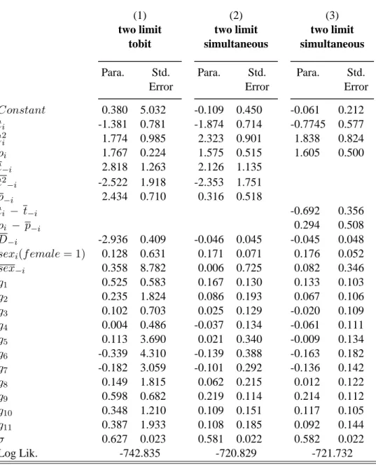
(35) the determinant of the corresponding matrix [Rkg × Rkg ]. Maximizing the log of (9) with respect to α and σ yields the full information maximum likelihood estimates of the model. Under standard regularity assumptions, these estimates are consistent and asymptotically efficient.. 5 Results Table 1 provides descriptive statistics of our sample. Most subjects are young and males are more numerous than females. Both tax rates and audit probabilities display a large standard deviation (see also Appendix B). This helps to identify their impact on tax compliance behavior. Over 88% (53/60) of all rounds with feedback information on the tax compliance satisfy the convergence criterion and therefore correspond to a social equilibrium. This leaves 795 observations on reported income in part II of the experiment (INFO treatment) out of 900 potential observations. In the INFO treatment, 24.5% of these observations (195) are censored at zero while 19% (151 observations) are censored at 100 for a total of 43.5% censored observations (346). The corresponding percentages in the NOINFO treatments are 18% (164 observations), 21% (189 observations) and 39% (353), respectively. Finally, the average reported income in the INFO treatment (50.15) is about half the initial endowment and slightly lower than the average reported income in the NOINFO treatment (53.92). Figures 1 and 2 compare the average reported income in both treatments according to individual tax rates and audit probabilities. Figure 1 shows that reported income increases slightly with individual tax rates up to 60%. Figure 2 shows that the reported income increases mostly as a function of individual audit probabilities. For a large majority of tax rates and audit probabilities the reported income is lower in the NOINFO treatment. These unconditional statistics need to be interpreted with care as they do not take into account other variables that have a direct effect on reported income. Table 2 reports detailed estimation results for various specifications of the model. As mentioned earlier the econometric results focus exclusively on the INFO treatment. Columns (1) and (2) provide results for the most general specification. They both correspond to a full linear-in-means model (but with censored variables) since individual and corresponding group mean variables are included as regressors. There are thus no exclusion restrictions on exogenous interactions variables. Correlated effects are taken into account through 11 group dummies. The tax rate variable, ti , is entered nonlinearly since our theoretical model predicts its impact on tax compliance can be decomposed into the sum of two opposite effects. Only a gender dummy is included in this specification since no other individual variable was significant at the 10 % level.. 14.

(36) Column (1) reports the estimation results for the general specification using a simple twolimit tobit. It thus ignores the possible simultaneity bias. Since there are only 15 participants in each session, this phenomenon may significantly bias the estimate of the endogenous social effect. Results from column (1) show that, contrary to expectations, the parameter estimate of D−i is negative and statistically significant at the 5% level. It translates into a marginal effect11 of -1.83. This is opposite to the social conformity effect because an increase in mean group tax evasion drives individuals to be more compliant. There are four reasons why such a result may obtain. First, tax evasion behavior may induce a social anti-conformity rather than a social conformity effect. In other words, participants may be inclined to deviate from the reference group’s behavior. Wenzel (2004) argues that, at least in the field of tax evasion, social norms may induce deviation from mean group response if the latter is inconsistent with individuals’ internal norms. Kooreman (2003) obtains such an anti-conformity effect when studying student self-esteem: the lower the group self-esteem, the higher the individual self-esteem. In our tax evasion experiment social anticonformity is unlikely, although it can not be completely ruled out. Second, since the tax yields are used to finance scientific research, altruistic behavior may induce individuals to contribute more when the others reduce their contribution. This explanation is also unlikely to explain much of the tax evasion behavior of the participants. A third interpretation is that individuals may reduce their tax evasion whenever the group evades more out of fear this may trigger a higher audit rate in further rounds. This is unlikely because audit regimes are exogenous and this was made common knowledge in the instructions. Finally, the most likely explanation is that the parameter estimate of D−i is biased because the simple two-limit tobit omits the potential simultaneity between individual and group responses. Recall that this bias may arise from the fact that individual and group behavior feed on each another. Moffitt (2001) and Krauth (2002) insist on the potential importance of this bias when the number of individuals in the reference group is small. The results reported in columns (2)–(6) are based on the likelihood function (9) and thus explicitly accounts for this. As it stands, the model in column (2) imposes no exclusion restrictions. Identification of the parameter estimates thus rests entirely on the response variables being censored and on the error terms assumed to be normally distributed. The first thing to notice is that the specifications of columns (2)–(6) all satisfy the coherency condition since the principal minors of the matrix I − Γ are positive in each case. This implies that there is no multiple equilibria in our experiment. In column (2) the parameter estimate of D−i , while still negative, is now much smaller (-0.046 rather than -2.936) and is no longer statistically significant (t = 1.02). This result is robust to changes in model specification and indicates that there is no endogenous interactions effects in our experiment. These results are consistent with the hypothesis that when the mean behavior of the group 11. We do not report marginal effects because they are intractable in specifications (2)–(6).. 15.

(37) does not affect the monetary payoffs of individuals, there is no endogenous social interactions associated with tax evasion (Spicer and Hero 1985).However, one must be cautious before generalizing this result to a real setting. Indeed, social interactions between players in a lab experiment are likely to be less strong than those between individuals from a same reference group in the real world. The model can easily be modified to investigate the existence of exogenous interactions. It suffices to include the tax rate and the audit probability both at the individual level, (ti ,pi ), and in deviation from group means, (ti − t−i , pi − p−i ), as in equation (4). Because the parameter estimate of (t2−i ) is not significant in specification (2) we have excluded it in specification (3) to ease interpretation. The parameter estimate of ti − t−i is negative and significant at the 5% level. This lends support to the existence of a fairness effect in terms of horizontal equity because individuals are inclined to report less when their fiscal treatment worsens relative to that of the group. Spicer and Becker (1980) have also found that individuals who were told their tax rates were above average reported relatively smaller amounts.12 On the other hand, the parameter estimate of pi − p−i is not significantly different from zero thereby rejecting fairness effects relative to the fraud preventing policy. According to the parameter estimates of ti and t2i in column (3), Yitzhaki’s prediction is verified at the mean tax rate (t¯ = 0.38). Indeed, a one percentage point increase in the individual tax rate increases desired reported income by as much as 0.622. The estimates also predict that the positive impact occurs only at tax rates above 21%. Below that level the negative effect dominates and induces more tax evasion. As discussed above, both positive and negative effects are consistent with our model when tax compliance yields a positive social marginal utility. Interestingly, experimental results on the impact of tax rates on compliance are not clear cut. Some studies have found that increased tax rates decrease compliance (Friedland et al 1978; Collins and Plumlee 1991), while others have found the converse to hold (Beck et al. 1991; Alm et al. 1995). In column (3) the parameter estimate of pi (= 1.605) is positive and significant at the 5% level. This result is consistent with the Alingham-Sandmo proposition, according to which an increase in the audit probability reduces tax evasion, but also with evidence based on survey data (Friedland et al. 1978; Beck et al. 1991, Slemrod et al. 2001). As in many studies, women are found to evade less than men (e.g., Spicer and Becker 1980, Baldry 1986). According to the parameter estimate of gender, ceteris paribus, females report on average 17.6 more units than males. As for correlated effects, only one group dummy (g9 ) is significant at the 10 % level. To test for the overall significance of correlated effects we re-estimated the model with no group dummies and report the results in columns (4). A likelihood ratio test based on columns (3) and (4) cannot reject the null assumption that all group dummies are 12. In an experiment similar to that of Spicer and Becker (1980), Webley et al. (1991) found no such fairness effect.. 16.

(38) zero (χ2 = 13.5 ∼ χ2 (11, .05) = 19.68). Our results are thus consistent with a fully randomized sample. However the mean group gender variable (sex−i ) is now significant at the 5% level so that gender composition is presumably correlated with group dummies. Column (5) reports estimation results where both endogenous effects and correlated effects are assumed away.13 Interestingly, the fairness effect on taxation is still significant at the 10% level and its value is close to the one obtained when both endogenous effects and correlated effects are included in the model (see column (3)). This result thus confirms the presence of exogenous effects in our experiment. Finally, column (6) includes our inequality aversion index (aversi ) and its average group counterpart into the model. As expected, its parameter estimate is positive and significant at the 5% level, thus indicating that those with a high inequality aversion are likely to evade less, ceteris paribus. Including this variable, however, has no impact on the other parameter estimates of the model.14. 6. Conclusion. Research on tax evasion usually ignores “peer effects” or “social interactions effects”. This omission is due to the fact that testing for such effects is notoriously difficult for two reasons. First, outcomes data rarely reveal the reference group composition, whether it is the family, the neighborhood, or work colleagues. Second, even when the group composition is known, estimating interaction-based models raises severe identification problems. The identification problem arises from the fact that interdependent behavior takes different forms that are difficult to isolate. The propensity of an individual to evade may genuinely vary according to the behavior of the group (endogenous interactions), but it may also vary with the exogenous characteristics of the group members (exogenous interactions). Further, correlated tax evasion outcomes need not arise from interdependent behavior alone. Indeed, members of a given group may behave similarly because they have similar individual characteristics or face similar institutional environments (correlated effects). In a simple linear-in-means regression-like model, equilibrium outcomes cannot distinguish endogenous effects from exogenous effects or correlated effects. Even when an interactions-based model is identified, its estimation raises serious econometric problems. In particular, the mean group decision, which appears as a regressor, is likely to be endogenous for two reasons. First, since individuals self-select within groups, they are likely to face common shocks and their observed and unobserved characteristics are likely to 13. This restriction can not be tested on the basis a log-likelihood ratio test since the two-limit tobit is not nested within our two-limit simultaneous tobit. 14 We also tested for “dynamic social learning effects” by including dummy variables for each round. None were ever significant at the 5% level.. 17.

(39) be highly correlated. Second, because individual and group behavior feed on one another, the two variables are potentially simultaneously determined, at least when the groups are small. In this paper we argue that laboratory experiments can be useful in solving these problems. Randomization of participants across groups limits correlated effects and sorting biases. Further, reference groups are naturally defined as participants in each particular session. This clearly helps identify the endogenous and exogenous interactions effects. The particular setup of our experiment has an added benefit. Because it generates censored data, it naturally implies a nonlinear relationship between individual and group responses, assuming normality of the error terms. This nonlinearity allows identification of the model without the need to impose any identifying restrictions. In line with the recent empirical literature on social interactions, we find that the estimation method is crucial in obtaining consistent estimates of interactions effects. Thus when we ignore the simultaneity of individual and group responses, we find strong evidence of social anti-conformity effects. These completely disappear once the simultaneity problem is taken into account using an appropriate estimation method (two-limit simultaneous tobit). We also find fairness effects in term of horizontal equity: for a same before-tax income, those with higher than mean group tax rate evade more in order to restore equity. Perceived unfair taxation may thus lead to increased tax evasion. At the policy level this means that a taxation system that is more horizontally equitable is likely to improve tax compliance. As noted by many (e.g., Manski 2000), experimental research also has its own limitations. In our experiment the groups of taxpayers are formed artificially for the sake of the experiment. Caution must thus be exercised when extrapolating our findings to the population of taxpayers.. 18.

(40) References [1] Akerlof, G.A. (1980). A Theory of Social Custom of Which Unemployment May be One Consequence. Quarterly Journal of Economics 94(4), 749-75. [2] Aaronson, D. (1998). Using Sibling Data to Estimate the Impact of Neigborhoods on Children’s Educational Outcomes. Journal of Human Resources 33, 915-46. [3] Allingham, M.G., Sandmo, A. (1972). Income Tax Evasion: A Theoretical Analysis. Journal of Public Economics 1, 323-38. [4] Alm, J., Jackson, B., McKee, M. (1992). Deterrence and Beyond: Toward a Kinder, Gentler IRS. In Slemrod, J. (Ed.), Tax Compliance and Tax Law Enforcement. Ann Arbor: University of Michigan Press, 311-32. [5] Amemiya, T. (1974). Multivariate Regression and Simultaneous Equation Model when the Dependent Variables are Truncated Normal, Econometrica, 6, 999-1012. [6] Alm, J., Sanchez, I., de Juan, A. (1995). Economic and Noneconomic Factors in Tax Compliance. Kyklos 48, 3-18. [7] Andreoni, J., Erard, B., Feinstein, J. (1998). Tax Compliance. Journal of Economic Literature 36(2), 818-60. [8] Aransson, T., Blomquist, S., Sacklen, H. (1999). Identifying Interdependent Behaviour in an Empirical Model of Labour Supply. Journal of Applied Econometrics 14(6), 60726. [9] Baldry, J.C. (1986). Tax Evasion is not a Gamble. Economics Letters 22, 333-5. [10] Beck, P.J., Davis, J.S., Jung, W. (1991). Experimental evidence on taxpayer reporting under uncertainty. The Accounting Review 66, 535-58. [11] Bosco, L., Mittone, L. (1997). Tax evasion and moral constraints: some experimental evidence. Kyklos 50, 297-324. [12] Brock, W.A., Durlauf, S.N. (2001a). Discrete Choice with Social Interactions. Review of Economic Studies 68, 235-60. [13] Brock, W.A., Durlauf, S.N. (2001b). Interactions-Based Models, in J. Heckman and E. Leamer, eds., Handbook of Econometrics 5, Elsevier Science B.V., 3297-380. [14] Collins, J.H., Plumlee, R.D. (1991). The taxpayer’s labor and reporting decision: The effect of audit schemes. The Accounting Review 66, 559-76. 19.

(41) [15] Elffers, H., Weigel, R.H. and Hessing, D.J. (1987). The Consequences of Different Strategies for Measuring Tax Evasion Behavior. Journal of Economic Psychology, 8, 311-37. [16] Erard, B., Feinstein, J.S. (1994). The Role of Moral Sentiments and Audits Perceptions in Tax Compliance. Public Finance/Finances Publiques 49 (Supplement), 70-89. [17] Evans, W.N., Oates, W. Schwab, R. (1992). Measuring Peer-Group Effects: Study of Teenage Behavior. Journal of Political Economy 100(5), 966-91. [18] Falk, A., Fischbacher, U. (2002). ”Crime” in the lab-detecting social interaction. European Economic Review 4, 859-69. [19] Falk, A., Fischbacher, U., Gächter, S. (2002). Isolating Social Interaction Effects- An Experimental Investigation. Working Paper, University of Zurich and University of St. Gallen. [20] Friedland, N., Maital, S., Rutenberg, A. (1978). A Simulation Study of Income Tax Evasion. Journal of Public Economics 10, 107-16. [21] Glaeser, E., Scheinkman J. (2000). Non-Market Interactions. National Bureau of Economic Research, Inc, NBER Working Paper 8053 2000. [22] Glaeser, E.J., Scheinkman, J., Sacerdote, B.I. (2003). The Social Multiplier. Journal of the European Economic Association 1 (2), 345-53. [23] Gordon, J.P.F. (1989). Individual Morality and Reputation Costs as Deterrents to Tax Evasion, European Economic Review 33, 797-805. [24] Gourieroux, C., Laffont, J.J., Monfort, A., (1980). Coherency Conditions in Simultaneous Linear Equation Models with Endogenous Switching Regimes, Econometrica 48(3), 675-95. [25] Kooreman, P. (2003). Time, Money, Peers, and Parents: Some Data and Theories on Teenage Behavior, IZA DP No. 931. [26] Krauth, B. (2002). Simulation-based estimation of peer effects. Working Paper, Simon Fraser University. [27] Manski, C.F. (1993). Identification of Endogenous Social Effects: The Reflection Problem. Review of Economic Studies 60(3), 531-42. [28] Manski, C.F. (2000). Economic Analysis of Social Interactions. Journal of Economic Perspectives 14(3), 115-36. 20.

(42) [29] Moffitt, R.A. (2001). Policy interventions, Low-Level Equilibria and Social Interactions, in S.N. Durlauf and H. Peyton Young (Eds.), Social Dynamics, Brookings Institution. [30] Myles, G.D., Naylor, R.A. (1996). A Model of Tax Evasion with Group Conformity and Social Customs. European Journal of Political Economy 12(1), 49-66. [31] Sheffrin, S.M., Triest, R.K. (1992). Can Brute Deterrence Backfire? Perceptions and Attitudes in Taxpayer Compliance. In Slemrod, J. (ed.), Tax Compliance and Tax Law Enforcement. Ann Arbor: University of Michigan Press, 193-218. [32] Shelling, T. (1978). Micromotives and Macrobehavior, New York: Norton. [33] Slemrod, J.B., Blumenthal, M., Christian, C. (2001). Taxpayer response to an increased probability of audit: evidence from a controlled experiment in Minnesota. Journal of Public Economics 79, 455-83. [34] Spicer, M., Becker, L.A. (1980). Fiscal Inequity and Tax Evasion: An Experimental Appoach. National Tax Journal 33(2), 171-5. [35] Spicer, M., Hero, R.E. (1985). Tax Evasion and Heuristics: A Research Note. Journal of Public Economics 26, 263-7. [36] Togler, B. (2002). Speaking to Theorists and Searching for Facts: Tax Morale and Tax Compliance in Experiments. Journal of Economic Surveys 16(15), 657-84. [37] Webley, P., Robben, H.S.J., Elffers, H., Hessing, D.J. (1991). Tax Evasion: The Experimental Approach. Cambridge: Cambridge University Press. [38] Wenzel, M. (2004). An Analysis of Norm Processes in Tax Compliance. Journal of Economic Psychology 25, 213-228. [39] Yitzhaki, S. (1974). A Note on Income Tax Evasion: A Theoretical Analysis. Journal of Public Economics 3, 201-2.. 21.

(43) Appendix A: Instructions You will be taking part in an experiment on decision-making under the aegis of both Université Laval in Québec and Université Lumière Lyon 2. The experiment is designed so that your earnings will depend on your decisions. The session consists of 10 rounds. The first five rounds involve a single-period, i.e. require a single decision. The next five rounds include several periods, with each period requiring one decision. In each round you will receive a score based on your decisions. The average score over entire session will determine your earnings. Scores are converted into Euros at the following rate: 100 experimental currency units = 15 e. In addition, you will receive a show-up fee of 1.5 e. Your earnings will be paid in cash at the end of the session in a separate room to preserve the confidentiality of your earnings. You will be part of a group of 15 participants from the same school. All your decisions are anonymous. Talking is not allowed throughout the entire session. Any violation of this rule will result in being excluded from the session and not receiving any payment. If you have any question regarding these instructions, please raise your hand; your question will be answered publicly. ROUNDS 1 to 5 Each round consists of a single period. At the beginning of each round, each participant receives an endowment of 100 experimental currency units . You are requested to give back a percentage of this endowment according to a “rate of deduction”. There are 5 different rates and each of these is randomly assigned to 3 participants. The sum of the deductions from the group members serves to finance scientific projects. The rate of reduction will be applied to the amount you report. You must use the scrollbar to report any amount between 0 and 100 (100 corresponding to the endowment that you received). This amount can be audited according to a certain audit probability and this audit may entail a penalty. There are 5 different audit probabilities and each of these is randomly assigned to 3 participants. The consequences of an audit are indicated below. There are 3 possible cases. • If the amount you report is not audited, your deduction rate will apply to your reported amount. In this case, no penalty applies. Your payoff is given by the following formula: Payoff = Deduction =. Endowment - Deduction Deduction rate × Reported amount. • If the amount you report is audited and is equal to your endowment, your deduction rate applies to this amount and consequently no penalty applies. Your payoff is given by the following formula: Payoff = Endowment - Deduction Deduction = Deduction rate × Endowment • If the amount you report is audited and is less than your endowment, your deduction rate applies to your endowment. In addition, you will be charged a penalty equal to your deduction rate times the non reported fraction of your endowment. Your payoff is then equivalent to: Payoff = Deduction = Penalty. =. Endowment - Deduction - Penalty Deduction rate × Endowment Deduction rate × Endowment - Reported amount. 22.

(44) What information do you receive at the beginning of each round? At the beginning of each round, you are informed about the following: • • • •. the 5 different deduction rates. your own deduction rate. the 5 different audit probabilities. your own audit probability.. On your computer screen you will find a scrollbar ranging from 0 to 100 which you must use to indicate the amount you wish to report. As you move the scrollbar, you will see both your payoffs if audited or not. To validate your decision, you must stop the scrollbar on the desired amount and then click the ”OK” button. Once all the participants have clicked the ”OK” button, the next round will begin automatically. You will be informed about the following at the end of the session only: • the actual audit of your reported amounts and the number of the rounds in which an audit actually took place. • the payment of a penalty when applicable. • your payoff. What changes from one round to the next ? Each round is independent from the previous ones. At the beginning of each new round, you will receive a new endowment of 100 experimental currency units. Likewise, new deduction rates and audit probabilities will be assigned randomly to participants. [T HE FOLLOWING INSTRUCTIONS WERE DISTRIBUTED TO THE PARTICIPANTS ONLY AFTER ROUND 5 WAS COMPLETED ]. ROUNDS 6 to 10 The session will continue in a moment, but with two changes however. 1. From now on, each round consists of several periods. At the beginning of each new period of a round, you will receive an endowment of 100 experimental currency units. Everyone keeps the same deduction rate and audit probability for all the periods of a given round. When a new round begins, new deduction rates and audit probabilities will be assigned randomly to all participants, including you. 2. As of the second period of a round, and for each successive periods, you will be given two additional pieces of information: • how many participants among the other 14 participants have reported less than their endowment in the preceding period. • the average amount reported by the other 14 participants in the preceding period.. 23.

(45) Appendix B: Values of tax rates and audit probabilities The values of the tax rates and the audit probabilities used in each session are the following: SESSIONS 1 TO 4 Distribution of the audit probabilities Regime Low Medium High. Individual Probability 0.04 0.07 0.24. 0.08 0.22 0.27. 0.11 0.27 0.33. 0.33 0.32 0.37. Mean. Standard Deviation. 0.18 0.25 0.33. 12.2 10.3 6.2. Mean 0.26 0.40 0.50. Standard Deviation 23.5 12 7. 0.37 0.37 0.43. Distribution of the tax rates Regime Low Medium High. 0.05 0.20 0.40. Individual tax rates 0.10 0.15 0.30 0.35 0.40 0.50 0.45 0.50 0.55. 0.70 0.55 0.60. SESSIONS 5 TO 8 Distribution of the audit probabilities Regime Low Medium High. 0.08 0.13 0.28. Individual Probability 0.12 0.15 0.37 0.27 0.32 0.37 0.30 0.37 0.40. 0.10 0.25 0.45. Individual tax rates 0.15 0.20 0.35 0.40 0.45 0.55 0.50 0.55 0.60. 0.41 0.42 0.47. Mean 0.23 0.30 0.36. Standard Deviation 13.6 9.95 6.89. Mean 0.31 0.45 0.55. Standard Deviation 23.54 12.25 7.07. Distribution of the tax rates Regime Low Medium High. 0.75 0.60 0.65. SESSIONS 9 TO 12 Distribution of the audit probabilities Regime Low Medium High. 0.02 0.03 0.20. Individual Probability 0.04 0.07 0.29 0.18 0.23 0.28 0.23 0.29 0.33. 0.33 0.33 0.40. Mean 0.15 0.21 0.29. Standard Deviation 13.22 10.29 7.13. Mean 0.24 0.35 0.45. Standard Deviation 21.54 12.25 7.07. Distribution of the tax rates Regime Low Medium High. 0.05 0.15 0.35. Individual tax rates 0.10 0.15 0.25 0.30 0.35 0.45 0.40 0.45 0.50. 24. 0.65 0.50 0.55.

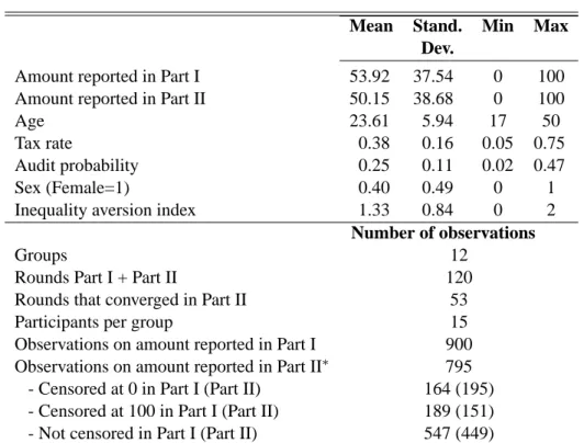
(46) Table 1 Descriptive Statistics Mean Amount reported in Part I Amount reported in Part II Age Tax rate Audit probability Sex (Female=1) Inequality aversion index Groups Rounds Part I + Part II Rounds that converged in Part II Participants per group Observations on amount reported in Part I Observations on amount reported in Part II∗ - Censored at 0 in Part I (Part II) - Censored at 100 in Part I (Part II) - Not censored in Part I (Part II) ∗ Observations are limited to games that converged.. 25. Stand. Dev.. Min. Max. 53.92 37.54 0 100 50.15 38.68 0 100 23.61 5.94 17 50 0.38 0.16 0.05 0.75 0.25 0.11 0.02 0.47 0.40 0.49 0 1 1.33 0.84 0 2 Number of observations 12 120 53 15 900 795 164 (195) 189 (151) 547 (449).

(47) Table 2 Estimation results of the structural form model of tax compliance (Dependent variable: Reported Individual divided by 100: Di /100). (1) two limit tobit Para. Constant ti t2i pi t−i t2 −i p−i ti − t−i pi − p−i D−i sexi (f emale = 1) sex−i g1 g2 g3 g4 g5 g6 g7 g8 g9 g10 g11 σ Log Lik.. 0.380 -1.381 1.774 1.767 2.818 -2.522 2.434. (2) two limit simultaneous. Std. Error. Para.. 5.032 0.781 0.985 0.224 1.263 1.918 0.710. -0.109 -1.874 2.323 1.575 2.126 -2.353 0.316. -2.936 0.409 0.128 0.631 0.358 8.782 0.525 0.583 0.235 1.824 0.102 0.703 0.004 0.486 0.113 3.690 -0.339 4.310 -0.182 3.059 0.149 1.815 0.598 0.682 0.348 1.210 0.387 1.933 0.627 0.023 -742.835. Std. Error 0.450 0.714 0.901 0.515 1.135 1.751 0.518. -0.046 0.045 0.171 0.071 0.006 0.725 0.167 0.130 0.086 0.193 0.025 0.129 -0.037 0.134 0.021 0.340 -0.139 0.388 -0.101 0.292 0.062 0.215 0.219 0.114 0.109 0.151 0.108 0.185 0.581 0.022 -720.829. Number of observations: 795. 26. (3) two limit simultaneous Para. -0.061 -0.7745 1.838 1.605. Std. Error 0.212 0.577 0.824 0.500. -0.692 0.356 0.294 0.508 -0.045 0.048 0.176 0.052 0.082 0.346 0.133 0.103 0.067 0.106 -0.020 0.109 -0.061 0.111 -0.009 0.134 -0.163 0.182 -0.136 0.142 0.012 0.122 0.214 0.112 0.117 0.105 0.092 0.144 0.582 0.022 -721.732.