Truth in Consequentiality: Theory and Field Evidence on Discrete Choice Experiments

Texte intégral

(1)2010s-43. Truth in Consequentiality: Theory and Field Evidence on Discrete Choice Experiments Christian A. Vossler, Maurice Doyon, Daniel Rondeau, Frédéric Roy-Vigneault. Série Scientifique Scientific Series. Montréal Octobre 2010. © 2010 Christian A. Vossler, Maurice Doyon, Daniel Rondeau, Frédéric Roy-Vigneault. Tous droits réservés. All rights reserved. Reproduction partielle permise avec citation du document source, incluant la notice ©. Short sections may be quoted without explicit permission, if full credit, including © notice, is given to the source..

(2) CIRANO Le CIRANO est un organisme sans but lucratif constitué en vertu de la Loi des compagnies du Québec. Le financement de son infrastructure et de ses activités de recherche provient des cotisations de ses organisations-membres, d’une subvention d’infrastructure du Ministère du Développement économique et régional et de la Recherche, de même que des subventions et mandats obtenus par ses équipes de recherche. CIRANO is a private non-profit organization incorporated under the Québec Companies Act. Its infrastructure and research activities are funded through fees paid by member organizations, an infrastructure grant from the Ministère du Développement économique et régional et de la Recherche, and grants and research mandates obtained by its research teams. Les partenaires du CIRANO Partenaire majeur Ministère du Développement économique, de l’Innovation et de l’Exportation Partenaires corporatifs Banque de développement du Canada Banque du Canada Banque Laurentienne du Canada Banque Nationale du Canada Banque Royale du Canada Banque Scotia Bell Canada BMO Groupe financier Caisse de dépôt et placement du Québec Fédération des caisses Desjardins du Québec Gaz Métro Hydro-Québec Industrie Canada Investissements PSP Ministère des Finances du Québec Power Corporation du Canada Raymond Chabot Grant Thornton Rio Tinto State Street Global Advisors Transat A.T. Ville de Montréal Partenaires universitaires École Polytechnique de Montréal HEC Montréal McGill University Université Concordia Université de Montréal Université de Sherbrooke Université du Québec Université du Québec à Montréal Université Laval Le CIRANO collabore avec de nombreux centres et chaires de recherche universitaires dont on peut consulter la liste sur son site web. Les cahiers de la série scientifique (CS) visent à rendre accessibles des résultats de recherche effectuée au CIRANO afin de susciter échanges et commentaires. Ces cahiers sont écrits dans le style des publications scientifiques. Les idées et les opinions émises sont sous l’unique responsabilité des auteurs et ne représentent pas nécessairement les positions du CIRANO ou de ses partenaires. This paper presents research carried out at CIRANO and aims at encouraging discussion and comment. The observations and viewpoints expressed are the sole responsibility of the authors. They do not necessarily represent positions of CIRANO or its partners.. ISSN 1198-8177. Partenaire financier.

(3) Truth in Consequentiality: Theory and Field Evidence on Discrete Choice Experiments* Christian A. Vossler†, Maurice Doyon‡, Daniel Rondeau§, Frédéric Roy-Vigneault** Résumé / Abstract Cette étude s’intéresse à des aspects méthodologiques associés à l’utilisation d’expériences avec choix discrets pour évaluer des biens publics. Nous avons développé un modèle explicite de jeux théoriques pour des décisions individuelles à des séries de choix, avec conditions générales sous lesquelles un questionnaire avec des choix binaires répétés incite la révélation des valeurs. Ce développement théorique est suivi d’expériences terrains avec traitements qui couvrent le spectre des incitatifs de la révélation des valeurs, passant de la décision avec mise en place réelle du projet et paiements réels de la part des participants, à celle sans aucune conséquence financière directe et avec projets hypothétiques. Les résultats indiquent qu’il est possible d’obtenir une révélation des valeurs réelles en situation hypothétique, si les participants pensent que leurs décisions ont un potentiel d’impact significatif sur une éventuelle politique. Mots clés : expériences avec choix discrets; expérience terrain; préférences révélées; conséquences, biais hypothétique. This paper explores methodological issues surrounding the use of discrete choice experiments to elicit values for public goods. We develop an explicit game-theoretic model of individual decisions to a series of choice sets, providing general conditions under which surveys with repeated binary choices are incentive compatible. We complement the theory with a framed field experiment, with treatments that span the spectrum from incentive compatible, financially binding decisions to decisions with no direct financial consequences. The results suggest truthful preference revelation is possible in surveys, provided that respondents view their decisions as having more than a weak chance of influencing policy. Keywords: discrete choice experiment, framed field experiment, mechanism design theory, stated preferences, consequentiality Codes JEL : C93, D72, D82, H41, Q51 *. We would like to acknowledge the financial support of AAFC and of CIRANO’s Sustainable Development research Group. We thank Laure Saulais for her help running the experiments, Michael Price, and seminar participants at the Fourth World Congress of Environmental and Resource Economists, the 2009 Southern Economic Association Meetings, and the University of Tennessee Faculties for their helpful comments and suggestions. † Department of Economics, University of Tennessee, Knoxville, Tennessee, USA. ‡ Département d'économie agroalimentaire et des sciences de la consommation, Université Laval, Québec City, Québec, Canada, email: Maurice.Doyon@eac.ulaval.ca. § Department of Economics, University of Victoria, Victoria, British Columbia, Canada, ** Département d'économie agroalimentaire, et des sciences de la consommation, Université Laval, Québec City, Québec, Canada..

(4) 1. Introduction Survey-based value elicitation methods have been a mainstay in various strands of research, including the non-market valuation of public goods, the study of transportation mode choice, estimating the value of a statistical life, and consumer product marketing. Most applications are for policy evaluation, and meeting Presidential Executive Orders for the last three decades has required the use of survey valuation methods in the context of benefit-cost analyses. Despite the widespread use of these methods, the influence of economic incentives on survey responses remains insufficiently understood. It is widely acknowledged that an essential component of stated preference surveys is conveying to participants that their responses have purpose. In practice, responses are commonly treated as reflecting truthful preferences or viewed as answers to purely hypothetical questions. Those with the former view may do so regardless of how values are elicited. Those with the latter view may dismiss the methodology entirely or advocate the use of “cheap talk” and related entreaty methods to convince respondents to behave as if incentives exist. Rather than adopt a particular perspective, we develop a game theoretic framework to analyze the incentive properties of the discrete choice experiment (DCE) approach to valuation, and we conduct a field experiment where the empirical evidence speaks in both favorable and unfavorable terms on the ability of DCE surveys to measure demand.1 Origins of DCEs lie in Lancaster’s (1966) theory of value and McFadden’s (1974) random utility theory. Closely related conjoint analysis applications in marketing and. 1. DCEs are also commonly referred to as “choice modeling”, “conjoint-based choice. experiments” or simply “choice experiments”. 2.

(5) transportation date back to at least the 1970s (e.g. Green and Rao, 1971; Norman and Louivere, 1974; Beggs, Cardell and Hausman, 1981), with DCEs gaining prominence in the 1980s (e.g. Louivere and Hensher, 1982) and applications in health economics and environmental economics beginning in the 1990s (e.g. Carson, Hanemann and Steinberg, 1990; Ryan and Hughes, 1997). Recent studies have used DCEs to compare the risk and time preferences of smokers and nonsmokers (Ida and Goto, 2009), estimate preferences for electricity reliability (Blass, Lach and Manski, 2010), and elicit discount rates for water quality policies (Viscusi, Huber and Bell, 2008). In a DCE, respondents are presented with a series of choice sets. Each set is made up of two or more comparable goods defined by their respective levels of common attributes, and respondents are asked to indicate the good they prefer. DCEs are often thought to be superior to alternative elicitation approaches, such as one-shot dichotomous choice, because of perceived gains in statistical efficiency; the ability to estimate the value of attributes at the margin, providing a richer depiction of preferences and facilitating benefits transfer studies; a reduction in some of the biases (e.g. “yea-saying”) through decreased focus on either providing or not providing a particular good; and the possibility of testing for internal consistency (Alpízar, Carlsson and Martinsson, 2001; Hanley, Mourato and Wright, 2001; Hanley, Wright and Adamowicz, 1998; Holmes and Adamowicz, 2003). Our study builds upon the theoretical insights of Carson and Groves (2007), and a handful of recent field and laboratory tests of criterion validity that compare a consequential stated preference measure and a revealed-preference criterion based on an incentive compatible mechanism. This literature represents a departure from the broader criterion validity research where purely hypothetical and inconsequential choices are the experimental counterpart to a. 3.

(6) stated preference survey. The two streams of literature suggest starkly different conclusions regarding the ability of stated preference surveys to truthfully reveal demand. The stylized fact from the broad literature is that there exists a positive and economically meaningful “hypothetical bias”, whereby people tend to overstate their values in hypothetical settings (List and Gallett, 2001; Little and Berrens, 2004; Murphy, Stevens and Weatherhead, 2005). On the other hand, when the focus is put on consequentiality of the survey, the evidence supports the view that one-shot dichotomous choice stated preference methods possess criterion validity (Carson et al., 2004; Johnston, 2006; Landry and List, 2007; Vossler and Evans, 2009; Vossler and Kerkvliet, 2003). Furthermore some studies have identified behavior in consequential (but non-incentive compatible elicitation settings) that is consistent with mechanism design theory predictions (Bateman et al., 2008; Carson et al., 2004; Polomé, 2003). In this study, we extend the existing theoretical and empirical literatures related to stated preference surveys in general and DCEs in particular. We develop an explicit game theoretic model of individual choice when participants are aware that they face multiple choices but where the mechanism by which individual decisions translate into the implementation of a public good can be explicit or unknown. The theory provides general conditions under which binary DCEs are incentive compatible. We show that for DCEs, incentive compatibility holds for a class of mechanisms that aggregate information in a way that maintains independence between choice sets and that meet specific monotonicity requirements (related to consequentiality). Unfortunately, in field surveys it is not possible to control the elicitation in a way that insures incentive compatibility, and we turn to empirics to gain insights on the ability of valuation surveys to reveal demand.. 4.

(7) In the empirical portion of the research, we conduct a framed field experiment that makes use of an opportunity to elicit values from local citizens for tree row plantations in agricultural areas of the province of Quebec (Canada). The field experiment represents the first criterion validity study involving a public good that compares values from an incentive compatible mechanism with that from an analogous advisory DCE survey. The baseline treatment involves an incentive compatible, financially binding DCE with a provision rule that makes clear that choice sets are independent. The next treatment involves a theoretically equivalent mechanism, but the provision rule does not make it absolutely clear that the independence condition holds. The third treatment involves a binding elicitation, but with no explicit provision rule. The last treatment is an advisory DCE that captures incentives in the field survey setting. In particular, there are no direct financial consequences of decisions and participants are informed that responses will be shared with policy makers but no information is given on how they will be used. Thus, overall, the experiment represents a continuum from which to explore the incentive properties of DCEs. We find that all three binding DCE treatments lead to statistically equivalent willingness to pay functions. The advisory DCE elicitation is not equivocal unless the sample is restricted to respondents who perceived that their choices had more than a “weak” chance of influencing policy. The empirical analysis suggests that truthful preference revelation is perhaps more likely than theory alone would suggest. However, only the subset of respondents who perceive their answers as consequential make choices similar to those in binding treatments. Hence, convincing respondents to stated preference surveys that their answers are consequential is critical to ensuring valid results.. 5.

(8) 2. Theoretical framework In this section we develop a theoretical framework for binary DCEs. In particular, we focus on a case where at most one policy/good can be provided, each choice set includes a status quo option, and the series of choice questions are disclosed in advance to respondents. This setup, while it does not encompass all forms of DCEs used in practice, fits many applications in environmental and health policy as well as recent field experiments in the marketing literature.2 We begin with the analysis of a tractable situation where there are direct financial consequences to the respondent and the provision rule is known. Once the fundamentals of this binding case have been established, the theory is extended to capture nuances of the stated preference, field survey setting. Our objective is to elaborate sufficient conditions to ensure that DCEs are incentive compatible. While these conditions are constructed around the theoretical arguments of Carson and Groves (2007), it is, to our knowledge, the first time that an explicit game theoretic model of individual choice in DCE’s has been put forth.. 2.1. Binding DCEs with full information about the policy function Consider a choice experiment with M participants each facing K choice sets where respondents are asked to indicate whether they prefer an alternative composed of a combination of attributes, or the status quo (no project being implemented). We refer to respondent’s choices as “votes”, a yes vote favoring the alternative in the choice set and a no vote favoring the status quo. Respondent i’s choices are represented by a vector Vi of length K, where each element. 2. In particular, we refer to Lusk and Schroeder (2006), and others who have recently used choice. experiments with direct financial consequences to analyze consumer preferences. 6.

(9) indicates a yes or no vote for one of the K choice sets. Denote the “policy function” as a vectorvalued function F : (V1 ,V2 ,...,VM ) → P = (P1 , P2 ,..., PK ) that maps the votes of all M respondents into a vector P of the probabilities that each of the K alternatives will be implemented. By construction, 0 ≤ Pk ≤ 1 ∀k , and. K. K. k =1. k =1. ∑ Pk ≤ 1 . The residual P0 = 1 − ∑ Pk is the probability that the. status quo is maintained. This policy function describes precisely how one’s vote affects the likelihood that each option will be implemented.3 The probability-based policy function is important in two ways. First, it acknowledges that there is uncertainty surrounding how one’s responses translate into the implementation of an alternative or of the status quo. Second, it makes it explicit that one’s choices interact with the choices of other respondents. From our perspective, these are two critical aspects of choice experiments that have often been overlooked. For a representative respondent, we denote the utility of the status quo by U0 , and the utility of alternative k by Uk = u(Y − ck ; A k ) . Y is the individual’s income, ck is the individual cost of the alternative and Ak is the vector of non-monetary attribute levels for choice k .4 It will be convenient to define U as the column transposition of the vector of utilities (U1 ,U2 ,...,UK ) to. 3. For a binding DCE, the function F (·) is simply the mechanism used to select from the real. project options presented in the DCE and the status quo. Later on, we consider uncertainty about the nature of F (·) both for binding DCEs as well as advisory DCEs. 4. While U0 and UK are meant to represent the utility of a single individual, the presentation does. not require that we maintain indices for different respondents.. 7.

(10) represent the utility levels that an individual would get from the implementation of each of the K possible alternatives. The agent’s expected utility from participating in the DCE is therefore given by. EU(V, V−m ) = F (V, V− m ) ⋅ U + P0U0. [1]. where V-m represents the votes of all other participants. For this model of choice to be appropriate, it is essential that agents meet the basic rationality requirements of expected utility. In particular, agents must be able to assign a utility level to each of the choice alternatives and to the status quo. This is not sufficient for DCE’s to be incentive compatible, however. Carson and Groves (2007) correctly state that survey instruments cannot be incentive compatible if they are not perceived to be consequential. In their words, consequentiality requires that 1) “agents answering a survey question must view their response as potentially influencing the agency’s action”; and 2) “the agent needs to care about what the outcomes of those actions might be” (p.183).. 2.1.1. Consequentiality In our context, the consequentiality of any vote requires that for each respondent, changing any single vote from a “no” to a “yes” affects the probability of implementation of at least one of the K alternatives in the DCE:5 ∆Pj ∆Vk ≠ 0 for at least one alternative j, for all k at least some of the time.. 5. [2]. Without loss of generality, we adopt the notational convention that ∆ Vj represents a change of. vote from “no” to “yes” on option j by a respondent. The negative, −∆Vj will represent a change from “yes” to “no”. 8.

(11) In other words, there has to be some probability that a participant’s votes will influence the outcome. This does not mean that every single vote must always have a direct marginal effect on the selection process. It could be, for instance, that F (·) relies on some form of majority rule in which a given participant’s choice may only be pivotal conditional on some combination of others’ votes. It is necessary, however, that each vote could be pivotal in some circumstances so that in expectation, each vote has the potential affect the outcome. Without [2], some or all of the votes have no influence (in expectation or in actuality) on the outcome, in which case, economic theory provides no guidance.. 2.1.2. Independence between choice sets With this framework in place, establishing the conditions for incentive compatibility requires a formal definition of the concept of independence between choice sets. We say that a policy function F (·) maintains independence between choice sets if ∆Pj ∆Vk = 0 ∀ j ≠ k . This condition simply means that if a participant were to change his vote on project k, the change can never have any impact on the probability that another outcome j will be implemented (where j excludes the status quo). When this condition is combined with the consequentiality condition [2], the DCE can only maintain independence and simultaneously be consequential if ∆Pk ∆Vk ≠ 0 in some circumstances, for all k. Proposition 1. Incentive Compatibility. If the policy function F (·) maintains independence between choice sets in a DCE, the DCE is incentive compatible in expected utility only if the probability of implementing a project k is. 9.

(12) monotonically increasing in the number of yes votes it receives: ∆Pk ∆Vk ≥ 0 ∀k , with strict monotonicity ∆Pk ∆Vk > 0 holding in some circumstances for all k.. Proof: Consider the votes of an individual and, without loss of generality, order the different options (including the status quo) according to the level of utility it confers to this individual. The respondent’s complete preference ordering will therefore take the form:. U1 ≥ U2 ≥ ... ≥ U0 ≥ ... ≥ UK and the column vector of utilities will be ordered accordingly (except for the absence of U0 ). Further define the demand revealing vector of votes V=T, in which option j receives a yes vote if and only if U j ≥ U0 (all others receive a no vote). The expected utility for a respondent, given his truth revealing vector and arbitrary votes by all other participants ( V−m ) is denoted by EU(T , V− m ) = F (T , V− m ) ⋅ U + P0U0 K K   = ∑ Fk (T , V− m ) Uk +  1 − ∑ Fk (T , V− m )  U0 k =1 k =1   .. [3]. The rest of the proof proceeds by establishing that T is a dominant strategy. Keeping V−m constant, consider any arbitrary variation V away from T. The resulting change in expected utility is then given by ∆EU = EU(V , V− m ) − EU(T , V− m ) K K  K  . = ∑ [Fk (V , V− m ) − Fk (T , V− m )] Uk +  ∑ Fk (T , V− m ) − ∑ Fk (V , V− m )  U0 k =1 k =1  k =1 . [4]. If F (·) maintains independence between choice sets, the effect of changing the vote on option j is strictly limited to modifying Pj and P0. Thus, equation [4] reduces to. 10.

(13) ∆EU = Fj (V , V− m ) − Fj (T , V− m ) U j + Fj (T , V− m ) − Fj (V , V− m ) U0 = ( Pj (V , V− m ) − Pj (T , V− m ))(U j − U0 ). .. [5]. If the initial vote in T was a yes, U j − U0 ≥ 0 and Pj (V , V− m ) − Pj (T , V− m ) ≤ 0 by virtue of the monotonicity assumption (∆Pj ∆Vj ≥ 0) . It follows that the change in expected utility from changing any yes vote to a no vote cannot increase the participant’s expected utility. By contrast, if the initial vote in T was a no, i.e. Uj ≤ U0 , the first term in equation [5] becomes positive, while the second is non-positive. Once again, deviating from true preferences cannot increase the participant’s expected utility. As long as the function F (·) maintains independence between choice sets, the impact on expected utility of changing several votes from T to V can always be reduced to the sum of the individual changes, just as demonstrated above. The impact of each individual change is always non-positive (no matter what the strategies adopted by other participants are). We can therefore conclude that truthful revelation is a dominant strategy. Truthful revelation is only weakly dominant if the mechanism does not maintain strict monotonicity (∆Pk ∆Vk > 0 ) everywhere or if U j = U 0 for one or more choice j. Absent these two sources of invariance, the demand revealing. strategy T is strictly dominant. Finally, if the mechanism maintains strict monotonicity and if the strict inequality in utilities holds for all players, the demand revealing strategy T by all participants constitutes a unique Nash Equilibrium of the choice experiment game. The independence assumption is critical to the result. If ∆Pj ∆Vk ≠ 0 , the costs and benefits of deviating from T for project j are no longer confined to changes in Pj and P0 . This gives rise to the possibility of trading expected benefits and costs across two or more projects and would result in optimal individual choices that are inconsistent with incentive compatibility. 11.

(14) 2.2. Binding DCEs with incomplete information about the policy function. In most policy-related DCEs, respondents are not given precise information about how their choices translate into policy or government action. It is therefore useful to consider how respondent uncertainty about the nature of the policy function F (·) might affect their incentives. One way of modeling this uncertainty is to postulate that respondents form beliefs about a range of possible policy functions and the probability that each will be implemented. In this context, the DCE can still be incentive compatible if i) the different policy functions considered by a respondent are mutually exclusive (only one policy function and one project can be implemented); ii) each possible policy function maintains independence between the choice sets; iii) all policy functions have ∆Pk ∆Vk ≥ 0 ∀k and at least one function meets all the monotonicity conditions required for consequentiality (in particular, that ∆Pk ∆Vk > 0 some of the time for all choice sets); and iv) at least one of the policy functions must be associated with a positive belief that it can be implemented. These sufficient conditions are strong enough that, even when the respondent considers the decisions of other participants, there is no strategic incentive to deviate from preference revelation for anyone who believes that these conditions hold. A participant could even conjecture that others have beliefs that are not consistent with the sufficient conditions and it would still be optimal for this participant to vote according to his preferences. In short, with beliefs that respect all conditions above, there is no possible strategic gain from misrepresenting one’s preferences. Of course, those holding beliefs that violate the conditions might not see it as optimal to reveal their preferences.. 12.

(15) As in the discussion of Carson and Groves (2007), the requirements simply ensure that participants will find it in their best interest to vote truthfully on all choice sets as long as they believe that a yes vote increases the likelihood of the option being implemented (with no chance of decreasing it).. 2.3. Advisory DCEs In the stated preference setting, participants are made aware that they are providing information on their preferences and are typically told that the information will be used by authorities to formulate policies. Such statements have the purpose of giving respondents a sense that their answers have consequences, presumably in the hope that it provides incentives for them to make careful choices that accurately reflects their preferences. As the scope of a DCE broadens from a setting with direct financial consequences and an unspecified policy rule to an advisory survey, even more details of the DCE are left to the interpretation of respondents. Respondents must form their own beliefs about a) how the experiment’s choice sets relate to the range of policies that may actually be devised; b) what their true cost to them might be; c) how the information provided affects the policy design; and d) how choices modify the likelihood that any policy will be implemented. Having worked through the binding DCE scenarios above, establishing the requirements for incentive compatibility in an advisory survey is relatively straightforward. The principal difference is that rather than working with a factual policy function, the analysis must proceed in the realm of respondent’s beliefs about possible policies and how their votes influence the policy maker’s decisions. If respondents form beliefs about how their choices influence a range of potential outcomes, they are once again required to form beliefs about the various policy. 13.

(16) functions that might be implemented. One important departure from a binding DCE with an unspecified rule, is that in an advisory survey, the range of possible policy outcomes that a participant might conjecture is as broad one’s imagination, much broader than the simple implementation of one of the options included in the choice sets. Under these circumstances, a DCE survey for general policy purposes will be incentive compatible if, in addition to maintaining the conditions laid out for a binding setting with incomplete information about the policy rule, the mapping from choice sets to the possible policy outcomes considered by a respondent must also maintain independence. As before, the basic thrust of the independence condition is that a respondent cannot believe that voting yes for a particular alternative changes the likelihood of implementation of other alternatives. Without independence, a vote on a single alternative expresses preferences about more than one alternative (or for certain combinations of attributes), potentially giving rise to non-truthful voting. Any deviation from one-to-one mapping between the choice sets presented in the experiment and the beliefs of a respondent about possible policy outcomes almost certainly violates the independence condition and incentive compatibility can no longer be guaranteed.. 2.4. Conditions for incentive compatibility in the field experiment We now discuss briefly conditions for incentive compatibility as they directly relate to the field experiment component of this study. In all of our experimental treatments, respondents were told that their choices would inform the development of policies by government agencies. In one treatment, there are no direct financial consequences and the conditions for incentive compatibility are those, discussed above, for an advisory DCE. In the remaining three treatments, participants’ choices had direct financial consequences and so two sources of incentives (direct. 14.

(17) and indirect) must be considered jointly. When choices have direct financial consequences as well as broader policy implications, a respondent’s vote must maximize K. B. EU(V , V− m ) = ∑∑ Pk (V , V− m )Pb (V , V− m ) u (Y − ck − cb ; Ak , Ab ) + P0,0U0. [6]. k =1 b =1. Where the subscripts, b, denotes (beliefs about) the broad policies that might be implemented, their attributes ( Ab ), cost ( cb ), and probability of implementation ( Pb ) as a function of the votes of all respondents. P0,0 is the probability that the status quo remains. For these treatments to be incentive compatible, one of following three conditions must hold in addition to the independence and monotonicity conditions. I. Beliefs about the policy outcomes Ab , cb and the mechanism generating Pb are identical to the actual choice sets (and probabilities of implementation) for real project implementation; II. The policy component is inconsequential (i.e. changing votes does not alter any Pb ) III. The real project component is inconsequential (i.e. changing votes does not alter any Pk ) In the first instance, any disparity between the policy options and the actual choice sets will almost certainly lead (if both are consequential) to a failure of the independence condition. To see this, note that changing a single vote on choice j affects the probability of true implementation Pj (and P0,0 ). Thus, all states of the world in which the joint probabilities includes Pj will be affected. Changing a vote on project j will have a marginal effect on the probability of implementing several public policies with differing attribute levels. It follows directly that independence cannot be maintained unless the choice sets presented to respondents. 15.

(18) maps directly and identically onto both the real project implementation and the policy consequences. The last two conditions simply reduce the situation to, respectively, the advisory and binding DCE cases we previously analyzed, in which either only the direct implementation or the policy implications affect the respondent’s decision, but not both. For an empirical survey with obvious measurement errors, it might be sufficient for “good measurements” that the direct implementation has a much greater marginal impact on the respondent’s utility function.. 3. Study design 3.1. Description of Projects and Choice Sets The field experiment component of this research is designed to provide insights on the issues of consequentiality and demand revelation in advisory DCEs. At its core is a survey instrument that elicits values for riparian and windbreak tree planting projects on agricultural land in the province of Quebec, Canada. This survey is part of a broader research effort to identify policies that enhance biodiversity, landscape amenities and provide soil erosion control in the region. Key project attributes and their relevant levels were identified through multiple pretests involving 140 individuals. Three attributes describe the tree planting projects: (1) Location, whether riparian (e.g. along a stream) or a as windbreak alongside a road); (2) Length, that is, the number of meters of streamside or roadside covered by the plantation; and (3) Width, the number of rows of trees to be planted. Table 1 presents the project attributes and their levels as well as the range of prices explored. The Location and Width attributes have 2 levels, the Length attribute has 3 levels, and. 16.

(19) the Cost or price attribute has 4 levels. The full factorial is thus 2x2x3x4 or 48. To reduce the total number of options, we generated 24 unique options using the SAS macro %mktex to enable identification of all main effects and two-way interactions (excluding Cost from the interactions) while maximizing D-efficiency. D-efficiency is 99%, and the design has perfect balance with respect to the non-price attributes, i.e. each of the possible 2x2x3 “projects” appear twice. By pairing each option with the status quo, there are 24 unique choice sets, and to reduce cognitive burden, these were separated into two blocks of 12 wherein each block included each unique project only once. Each participant received one block of 12 choice sets. Thus, to be clear, each participant voted on each project once, and only the project prices differed across participants. To remain consistent with field survey settings, the fact that different participants saw different prices was not common knowledge. The choice sets were presented as binary referenda where a “yes” vote is a choice for the tree planting project and a “no” vote is a choice for no tree planting project (i.e. the status quo).. 3.2. Experiment treatments The study is divided into four experimental treatments. In three of them, participants have the direct opportunity to fund an actual tree planting project through their choices with their own money. Two of these three treatments are designed to be theoretically incentive compatible if any influence of choices on broader policy issues are ignored. In the fourth treatment, participants cannot directly finance tree projects and no project can be implemented as a direct result of their choices. The ordering of the treatments mirrors the development of the theory, and accordingly, reflects expectations of the likelihood the elicitation is demand revealing.. 17.

(20) 3.2.1. Binding DCE, Independent Lottery Provision Rule (B-IL) In this treatment, respondents’ votes probabilistically lead to the implementation of one of the 12 projects, or the status quo. Participants are instructed that one of the 12 choice sets will be randomly chosen at the end of the experiment, each with equal probability. This random selection procedure was chosen to make clear to participants that choice sets are independent. For the selected choice set, the proportion of yes votes among all participants is computed. A second draw is then performed to choose between the status quo and the implementation of the project. In this second draw, the real project is implemented with a probability equal to the proportion of yes votes it received. This probabilistic implementation rule is superior to a common majority-vote rule in that it provides incentives to all participants by eliminating the possibility that one might perceive his vote to be non-pivotal, i.e. the provision rule imposes strict monotonicity. In execution, one of the 12 choice sets is selected by rolling a 12-sided die. Two 10-sided dice are used to obtain a number between 0 and 99, this number is then the “acceptance level”. If the percentage of yes vote equals or exceeds the acceptance level, the project is accepted and each participant must pay his individual cost amount. The selected project, as described, will then be undertaken. Otherwise, no money is collected and no tree project is carried out. If we record a yes vote on project k by respondent i as Vik = 1 , a no vote as Vik = 0 and if M N N N N we define Nk = ∑ Vmk , the mechanism takes the form F ( V , V− m ) =  1 , 2 ,..., k ,..., K  , KM KM   KM KM m =1 where KM is the total number of votes cast. If beliefs about possible government policies are consistent with the choice sets (Condition I) or if the broader government policy implications are inconsequential (Condition II - or considered much less important than the real and immediately. 18.

(21) costly project implementations), then ∆Pk ∆Vk > 0 ∀k . By Proposition 1, this mechanism is incentive compatible and truthful revelation of demand a dominant strategy.. 3.2.2. Binding DCE, Aggregate Lottery Provision Rule (B-AL) In the second treatment, each vote for a particular option (whether a project or the status quo) directly maps into the probability the option is implemented. This is made operational by assigning each of the 12 projects, and the status quo, a separate color. Each participant’s yes vote adds one poker chip of the corresponding color to a bag. A no vote, favoring the status quo, adds a black colored chip. After all votes are cast, the bag is filled with (N1 , N2 ,..., NK ) of the K different K   colored chips, and  KM − ∑ N j  black chips (for a total of KM chips). The option to be k =1  . implemented is determined by a single draw from the bag. If a colored chip is drawn, the corresponding project is implemented. If a black chip is drawn, the status quo prevails. With this implementation procedure, it follows that the probability that project k is implemented is once again given by Nk KM , and the policy function is identical to that of the BIL treatment. It is similarly incentive compatible with truthful demand revelation as a strictly dominant strategy if we abstract from broader policy implications, i.e. if condition (I) or condition (II) hold. However, as votes for all choice sets are considered in the aggregation process, we posit that it is less obvious to participants that the independence property indeed holds.. 19.

(22) 3.2.3. Binding DCE, Undisclosed Provision Rule (B-U) In the third treatment, participants are informed that their choices will be used to determine which option will be implemented, i.e. the elicitation is consequential and there are direct financial consequences. However, no description of the provision rule was provided to participants. As such, participants were free to form beliefs about how an option might be chosen and how their votes could influence this choice. Without additional precision on the provision rule, there can be no guarantee that independence is maintained or that the mechanism is incentive compatible even when the direct financial component is considered in isolation. In practice, one of the 12 choice sets was selected at random using a 12-sided die, and a simple majority-vote rule decided whether the particular project would be carried out not.. 3.2.4. Advisory DCE (A) The last treatment is a non-binding, stated preference DCE wherein participants voted on 12 projects without direct financial consequences. As in other treatments, participants were told that the results of the study would be provided to a government agency. To the extent that they believe that their choices can influence actual policy decisions, this too would be a consequential elicitation. Even so, however, as discussed in the theory section, it is probable that at least some participants might form beliefs (about the way in which the information will be used) that do not maintain the desirable assumption of independence between choice sets.. 3.3. Experiment Protocol and Survey Description Aside from the particular provision rule, and associated financial incentives, the experimental protocol was identical across all treatments. Participants were given a show-up. 20.

(23) payment of C$100 (100 Canadian Dollars) in the real payment treatments and C$50 in the advisory DCE.6 The show-up payments differed in this fashion in attempt to, based on our pilot data, equate expected earnings across treatments. Experiment instructions were presented using a PowerPoint presentation (available upon request) by the same moderator. The presentation slides included a brief introduction of the study, descriptions and computer-edited before and after photographs illustrating the tree projects and attribute levels that that participants would vote on, and, in the case of the binding DCEs, two examples illustrating the implementation mechanism. Participants also had a paper copy of the photographs and a description of the benefits of riparian and windbreaker tree plantings. Participants were informed that their surveys would be shared with policy makers, but that anonymity would be maintained. For a particular treatment, six versions of the survey were randomly assigned to participants to be completed using a pencil. The versions differ by the order of the choice sets to control for possible order effects, and by the different price vectors. Aside from the discussion of provision rules, the process closely parallels a field survey. In the first section of the survey, participants are asked questions that elicit participants’ attitudes on environmental issues. The second section contains the DCE. The third section asked typical demographic questions, in addition to questions intended to gauge strategic voting and consequentiality.. 6. The payment was given in cash upon arrival. Participants were told orally and in writing that. this money was theirs to keep and informed that they are free to leave at any moment and still retain the show-up payment. Two participants choose to leave with the show-up fee without completing the study. 21.

(24) 3.4 Participants Participants were volunteer adults recruited through a mailing list of Laval University employees and friends of Laval, as well as through the mailing list of the Institut des Nutraceutiques et des Aliments Fonctionnels (INAF).7 These lists included roughly 5000 people who have expressed an interest in receiving news from Laval University or INAF. Participants needed to be at least 18 years old and could only participate once. Eight sessions, two for each treatment, took place between March and June 2009 in the INAF building located in Quebec City. Volunteers were randomly assigned into treatment, which makes possible the identification of treatment effects. Two hundred and twenty participants completed the experiment, with a roughly equal number of participants in the four treatments: 58, 55, 52, and 55 respectively. Three projects were implemented as the result of votes in the six binding DCE sessions: a 1 km by 3 rows windbreaker, a 1 km by 1 row windbreaker, and a riparian band of 1km by 3 rows. Table 2 presents some basic demographic information on our participants. We note that the demographics are similar across treatments (detailed information available upon request). Overall, the average participant has a higher household income and is better educated than the general population of Quebec. The age distribution (and average age), employment rate, and percentage of males are similar. As the primary goal of the study is to provide insight on. 7. For the advisory DCE treatment people were recruited by announcing a C$50 participation. payment. For the other treatments, participants were recruited by announcing an expected gain of C$50 with the mention that the amount might be greater or lower, depending of the outcome of the session. 22.

(25) important methodological issues, we make no claims regarding the suitability of our results as population estimates.. 4. Results 4.1 Analysis of Willingness to Pay We begin our analysis with the estimation of a WTP regression based on the maximum likelihood estimator of Cameron and James (1987). In particular, we treat willingness to pay as a censored dependent variable for which we obtain the signal WTPt ,ik ≥ ct ,ik if, in treatment t, participant i votes “yes” to cost ct,ik associated with a project k, or the signal WTPt ,ik < ct ,ik if participant i votes “no”. Let WTPt,ik be a linear function of a column vector of covariates, xt,ik, such that WTPt ,ik = xt ,ik' β t + ε t ,ik , where β t is a column vector of unknown parameters and ε t ,ik is a normally distributed mean-zero error term with treatment-specific standard deviation σt. Let yt,ik = 1 denote a “yes” vote and yt,ik = 0 indicate a “no” vote. Further, denote It ,ik as an indicator variable that equals 1 if participant i faces treatment t and equals 0 otherwise. Then, the log-likelihood function is. N. ln L =. K. ∑∑ i =1 k =1.    yik ln  .     c − x ′β 1-Φ  t ,ik4 t ,ik t    ∑ It ,ikσ t   t =1 .      c − x ′β    + (1 − yik )ln Φ  t ,ik4 t ,ik t    It ,ikσ t    ∑ t =1  .        .      . [7]. Assuming the error term has a normal distribution here is analogous to assuming a normal distribution for WTP.. 23.

(26) Included as covariates are project attributes, as well as control variables that correspond with household size, income and attainment of a graduate degree.8 To control for unmeasured factors specific to an individual we estimate cluster-robust standard errors. With our functional form and error distribution assumption, interpretation of estimated parameters is analogous to that of a standard linear regression model that treats WTP as a directly observed (i.e. uncensored) dependent variable. 9 The first set of estimation results presented in Table 3 uses the full sample of 220 participants. Estimation is by means of a user-defined maximum likelihood procedure programmed by the authors in Stata. The overall model results suggest that, in all treatments, the estimated marginal WTP for the Length, Width, and Location attributes are statistically significant (beyond the 1% level) and economically meaningful. For instance, ceteris paribus, the estimated WTP function for the B-IL treatment suggests that participants are willing to pay about C$0.04 for every one-meter increase in length (or C$4 for a 100m increase), C$12.48 for an additional row of trees and an additional C$9.75 if the tree planting is in a riparian area. This suggests a high total WTP for many of the tree projects offered to respondents. As further evidence of construct validity, those with higher income and education (the latter effect is only. 8. In our initial specification we included all demographic variables defined in Table 2, as well as. interactions between all project attributes. The more parsimonious specification we present is justified by statistical tests. No conclusion we reach is sensitive to the inclusion/exclusion of these other covariates. 9. We also explored the logistic, log-logistic, log-normal and Weibull distributions for the error. term. Our statistical conclusions appear robust to the distributional assumption. 24.

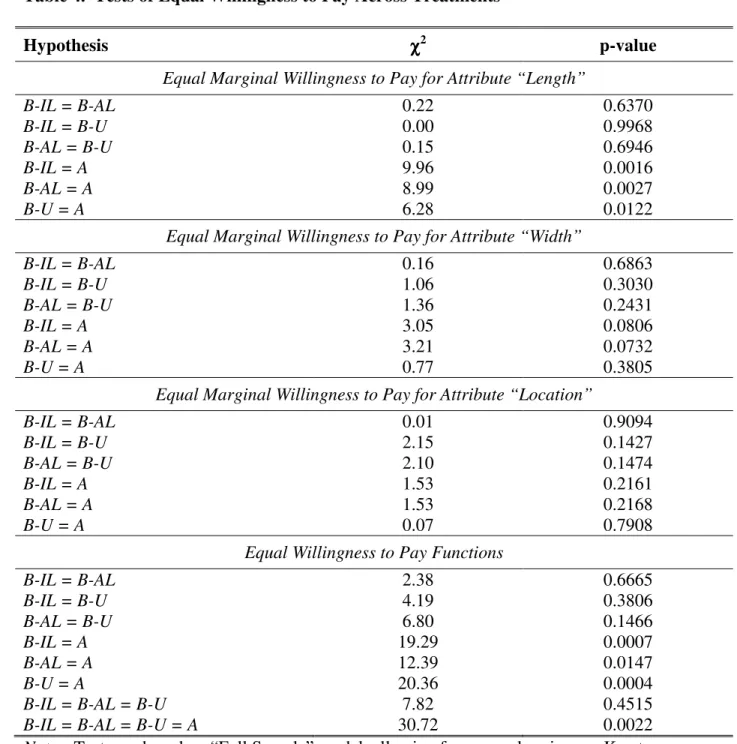
(27) significant at the 7% significance level) are willing to pay more for tree plantings, whereas participants with larger households (which likely reflects higher demands on household income) are willing to pay less. The standard deviation of WTP is the lowest for the B-IL treatment, which is hypothesized to be the most transparent in terms of its incentives. Relative to the B-IL treatment, the scale for the other three treatments is statistically different, and in particular is about 50% higher in the B-U and A treatments, and about 70% higher in the B-AL treatment. This is evidence that the less transparent treatments are associated with significantly more behavioral noise. Applying a standard Wald test to the “Full Sample” model, we tested for equality in the marginal WTP of program attributes across treatments as well as for equal overall WTP functions (in particular, equal marginal WTP for all attributes as well as an identical intercept). The results of these tests, details of which are presented in Table 4, can be succinctly summarized as follows: (i) the binding DCE treatments elicited statistically indistinguishable WTP functions; and (ii) the advisory DCE function is statistically different form that of any other treatment. Examining the test results a bit closer, for each possible pairwise test involving two binding DCE treatments, we fail to reject the null hypothesis of equal marginal WTP for any attribute, even at the 10% level. Indeed, we fail to reject the null hypothesis that all three WTP functions are identical. In contrast, marginal WTP for Length and Width tends to be statistically higher for the advisory DCE. To put this into perspective, for a moderate-level project (Length = 600; Rows=3; Location=0), estimated mean WTP from the B-IL function is C$45.73 whereas it is C$60.31 using the advisory DCE function (a 32% increase).. 25.

(28) 4.2. Survey evidence 4.2.1. Strategic voting In treatments B-IL and B-AL, Proposition 1 holds as a result of the particular (and disclosed) provision rule used. However, unless condition (I) or (II) is satisfied, the elicitation mechanisms are not incentive compatible. Further, as discussed in the theory section, very strong assumptions are needed for the incentive compatibility of treatment B-U as well as the advisory DCE. As (perceived) non-independence of a participant’s voting choices could give rise to strategic voting and subsequent non-incentive compatibility, we included a survey question to measure the effect of strategic considerations on voting. In particular, we asked participants – after they had voted but before the outcome (if any) was announced – whether they had considered how other participants might vote the choices of other people in the group when voting, and if so, to indicate how many of their own votes were affected by the consideration of others’ votes. Responses to the survey question, by treatment, are presented in Table 5. The most striking is the advisory DCE where just one respondent provided an indication of strategic voting. There is some stated evidence of strategic voting in the B-IL and B-AL treatments, where roughly 10% indicated that strategic motivations affected two or more votes. The most support of strategic voting is for the B-U treatment, where 25% indicated strategic voting. However, the impact of strategic voting appears to be modest at best for this treatment, as less than 6% suggested that strategic considerations altered three or more votes and just one of these respondents indicated it had affected more than five votes. Using pair-wise KomolgorovSmirnov Tests, we fail to reject the null hypothesis of equal response distributions in all cases. As a robustness check, we re-estimated equation [7] while excluding any participant with stated. 26.

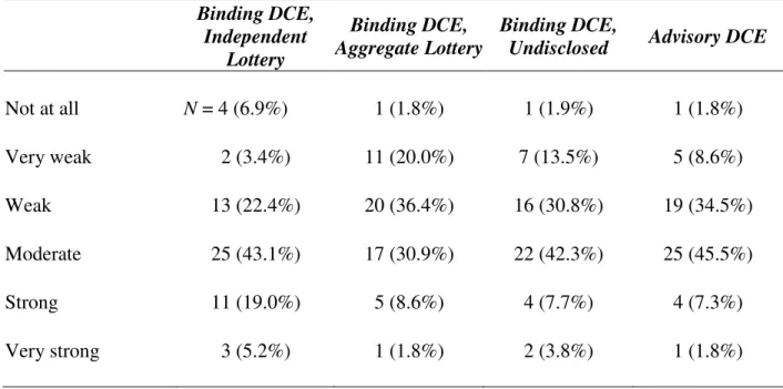
(29) evidence of strategic voting. All of our findings remain. The overall evidence suggests that while some strategic voting is present in the binding treatments, the resulting bias is negligible.. 4.2.2 Indirect consequences Contrary to the binding DCE treatments, a necessary condition for incentive compatibility of the advisory DCE is that respondents perceive their votes to have some potential influence on public policy. The question we asked all respondents (after they had voted), roughly translated from French, is “To what extent do you believe that your votes will be taken into account by the authorities?” The six response categories, and the number of respondents that selected each are presented as Table 6. As indirect consequences in the advisory DCE are essential to incentive compatibility, we explored whether elicited preferences depend on this. In particular, we re-estimated the model defined by equation [7] with restricted samples. In our first pass, we excluded the six advisory DCE respondents who perceived their responses to have, at most, a very weak influence. This had little effect, which is not surprising given this excluded only 11% of the advisory DCE sample. Second, we excluded the 25 respondents who perceived their influence to be weak at best. We present the resultant “Restricted Sample” model in Table 3. Using Wald tests, with the restricted sample, we fail to reject equality between the advisory DCE WTP function and any of the three binding DCE functions: B-IL=A (χ2=5.47, p=0.2421); B-AL=A (χ2=4.89, p=0.2992); B-U=A (χ2=7.20, p=0.1255). Further, as the decrease in sample size leads to a less powerful test, we estimated another model that restricted the real payment WTP to be equal (recall these restrictions were supported) and still likewise fail to reject equality between the (pooled) binding DCE function and the advisory DCE function. 27.

(30) (χ2=6.10, p=0.1918). We note that each WTP function coefficient corresponding with the advisory DCE moves closer to those from the B-IL and B-AL treatments when using the restricted sample. This provides additional evidence that the equality of WTP functions is not purely a function of the reduction in sample size. To put this into perspective, for a moderatelevel project (Length = 600; Rows=3; Location=0 - roadside), estimated mean WTP from the BIL function in the “Restricted Sample” model is C$46.10 whereas it is C$54.50 using the advisory DCE function. This difference is not statistically significant (χ2=1.82, p=0.177). To provide (further) empirical evidence that condition (I) or (II) holds for the binding DCE treatments, we re-estimated equation [7] but allowed all the attribute-related coefficients as well as the intercepts to vary between those who perceived the indirect incentives to be strong and those who perceived otherwise. Based on the cutoff point described above, we fail to reject equality of equal WTP functions across subgroups for any of the binding DCE treatments: B-IL (χ2=7.04, p=0.1339); B-AL (χ2=6.87, p=0.1430); B-U (χ2=2.22, p=0.6961). We can (marginally) reject that the WTP functions are equal across subgroups for the advisory DCE (χ2=8.48, p=0.0754).. 5. Discussion From a mechanism design perspective, using a stated preference, advisory DCE to truthfully elicit preferences for public goods is a dubious task. Generally speaking, as derived in this paper, incentive compatibility requires respondents to believe that decisions are consequential and furthermore, that policy makers use the information in such a way that maintains choice set independence. In the field survey setting these beliefs cannot be directly observed or conclusively controlled for and it is quite simple to construct any number of belief. 28.

(31) systems that fail the test of incentive compatibility. The evidence from our field experiment, nevertheless, suggests that independence is rarely violated, and that consistent preference revelation is possible if we restrict the sample to those who perceived that their responses had more than a weak impact on policy. We note that when no restrictions on the sample are made, however, the magnitude of the bias is modest and is between 32-43% across the range of tree planting projects we investigate. Why not vote strategically in an advisory DCE? We have no definitive answer but it is at least plausible that the complication of the decision task strains the cognitive resources of participants; or perhaps, that the policy process is sufficiently opaque to respondents that their beliefs about the policy process remain closely tied the options presented to them in the survey material and choice experiment itself. If this were true, it would signal that stated preference methods can indeed be considered credible by respondents and produce quality data. There is a word of caution in broadly interpreting our evidence as it is possible that strategic voting occurs in other settings, such as when three or more options are included in a choice set or when preferences for private goods are elicited. Theoretical assumptions for incentive compatibility are much more substantive in such settings, and it is unclear to what extent theoretical shortcomings translate into empirical results. A main take home message from this study is that, even in an advisory survey where financial incentives are indirect and remote, incentives do indeed exist. However, at least if we take at face value the stated perceptions regarding the consequences of the advisory DCE, our findings suggest that respondents must perceive there to be higher than merely an epsilon chance that the elicitation has consequences. This finding contrasts the sharper empirical results in the existing literature (e.g. Herriges et al., 2010), but nevertheless highlights the importance of. 29.

(32) consequentiality and the potential value in including pertinent survey questions. The evidence lends support to the view that the notion of consequentiality is more important than the “real vs. hypothetical” type of comparison commonly used in determining the criterion validity of an advisory survey. In an attempt to identify factors correlated with consequentialism, we modeled the categorical choices to our consequentiality question using an ordered probit model. Including the variables described in Table 2 as well as treatment indicators as covariates, we uncovered very little. The only statistically significant factor was whether the participant gave money to charity in the past year, with those doing so selecting roughly one category lower (less consequential), on average. It is plausible that those giving to charity are more likely to question the ability of the government to undertake action. By all accounts, further exploration into respondent perceptions regarding the consequences of advisory surveys is warranted.. 30.

(33) References Alpízar, Francisco, Fredrik Carlsson, Peter Martinsson, 2001. Using choice experiments for nonmarket valuation, Economic Issues 8, 83-110. Bateman, Ian J., Richard T. Carson, Brett Day, Diane Dupont, Jordan J. Louviere, Sanae Morimoto, Riccardo Scarpa and Paul Wang, 2008. Choice set awareness and ordering effects in discrete choice experiments, Working paper, University of East Anglia, UK. Beggs, S., S. Cardell and J. Hausman, 1981. Assessing the potential demand for electric cars, Journal of Econometrics 17, 1-19. Blass, Asher, Saul Lach and Charles F. Manski, 2010. Using elicited choice probabilities to estimate random utility models: Preferences for electricity reliability, International Economic Review 51, 421-440. Cameron, Trudy A. and Michelle D. James, 1987. Efficient estimation methods for use with “closed-ended” contingent valuation survey data, Review of Economics and Statistics 69, 269-276. Carson, Richard and Theodore Groves, 2007. Incentive and information properties of preference questions, Environmental & Resource Economics 37, 181-210. Carson, Richard, Theodore Groves, John List and Mark Machina, 2004. Probabilistic influence and supplemental benefits: a field test of the two key assumptions underlying stated preferences, Working Paper, Department of Economics, University of California, San Diego. Carson, Richard, Michael Hanemann and Dan Steinberg, 1990. A discrete choice contingent valuation estimate of the value of Kenai King Salmon, Journal of Behavioral Economics, 19, 53-68.. 31.

(34) Green, Paul E. and Vithala R. Rao, 1971. Conjoint measurement for quantifying judgmental data, Journal of Marketing Research 8, 355-363. Hanley, Nick, Susana Mourato and Robert E. Wright, 2001. Choice modelling approaches: a superior alternative for environmental valuation?, Journal of Economic Surveys 15, 435462. Hanley, Nick, Robert E. Wright and Wiktor Adamowicz, 1998. Using choice experiments to value the environment: design issues, current experience and future prospects, Environmental & Resource Economics 11, 413-428. Herriges, Joseph, Catherine Kling, Chih-Chen Liu and Justin Tobias, 2010. What are the consequences of consequentiality?, Journal of Environmental Economics and Management 59, 67-81. Holmes, Thomas P. and Wiktor L. Adamowicz, 2003. Attribute-based methods, in K.J. Boyle and P.A. Champ (Eds.), A primer on non-market valuation, Kluwer Academic Publishers, Boston. Ida, Takanori and Rei Goto, 2009. Simultaneous measurement of time and risk preferences: Stated preference discrete choice modeling analysis depending on smoking behavior, International Economic Review 50, 1169-1182. Johnston, Robert J., 2006. Is hypothetical bias universal? Validating contingent valuation responses using a binding public referendum, Journal of Environmental Economics and Management 52, 469-481. Lancaster, Kelvin J., 1966. A new approach to consumer theory, Journal of Political Economy 74, 132-157.. 32.

(35) Landry, Craig E. and John A. List, 2007. Using ex ante approaches to obtain credible signals for value in contingent markets: evidence from the field, American Journal of Agricultural Economics 89, 420-432. List, John A. and Craig A. Gallet, 2001. What experimental protocol influence disparities between actual and hypothetical stated values? Evidence from a meta-analysis, Environmental & Resource Economics 20, 241-254. Little, Joseph and Robert Berrens, 2004. Explaining disparities between actual and hypothetical stated values: further investigation using meta-analysis, Economics Bulletin 3, 1-13. Louviere, Jordan J. and Daniel Hensher, 1982. On the design and analysis of simulated choice or allocation experiments in travel choice modelling, Transportation Research Record 890, 11-17. Lusk, Jayson L. and Ted C. Schroeder, 2006. Auction bids and shopping choices, Advances in Economic Analysis & Policy 6, Article 4. McFadden, Daniel, 1974. Conditional Logit Analysis of Qualitative Choice Behavior, in P. Zarembka (Ed.), Frontiers in Econometrics, Academic Press, New York. Murphy, James J., Thomas H. Stevens, Darryl Weatherhead, 2005. A meta-analysis of hypothetical bias in contingent valuation, Environmental & Resource Economics 30, 313325. Norman, K. and Jordan Louviere, 1974. Integration of attributes in public bus transportation: Two Modeling Approaches, Journal of Applied Psychology 59, 753-758. Polomé, Philipe, 2003. Experimental evidence on deliberate misrepresentation in referendum contingent valuation, Journal of Economic Behavior & Organization 52, 387-401.. 33.

(36) Ryan, Mandy and Jenny Hughes, 1997. Using conjoint analysis to assess women's preferences for miscarriage management, Health Economics 6, 261-73. Viscusi, W. Kip, Joel Huber and Jason Bell, 2008. Estimating discount rates for environmental quality from utility-based choice experiments, Journal of Risk and Uncertainty 37, 199220. Vossler, Christian A. and Mary F. Evans, 2009. Bridging the gap between the field and the lab: environmental goods, policy maker input, and consequentiality, Journal of Environmental Economics and Management 58, 338-345. Vossler, Christian A. and Joe Kerkvliet, 2003. A criterion validity test of the contingent valuation method: comparing hypothetical and actual voting behavior for a public referendum, Journal of Environmental Economics and Management 45, 631-649.. 34.

(37) Table 1. Discrete Choice Experiment Attributes and Levels Attribute. Description. Levels. Length. Length of tree planting, in meters. 300 600 1000. Width. Number of rows in tree planting. 1 3. Location. Location of tree planting. Riparian (along stream or river) Windbreak (along roadside). Cost of tree planting, in C$. 10 25 50 75. Cost. 35.

(38) Table 2. Descriptive Statistics Variable Name. Description. Gender. % Male. Sample Mean (Std. Dev.) 45.00 (49.86). Age. Age, in years. 40.30 (13.80). College Degree. % with college degree or higher. 62.27 (48.58). Graduate Degree. % with graduate degree. 35.45 (47.95). Employment. 77.27 (42.00). Environmental. % currently employed Household income, in C$ 1000s; the midpoint of the category chosen by the respondent is used % members of an environmental organization. Household Size. Number currently living in the household. 2.57 (1.45). Charity. % indicating a donation to charity in past 12 months. 82.27 (32.28). Income. 36. 62.34 (40.58) 6.82 (25.26).

(39) Table 3. Willingness to Pay Regressions Full Sample. Restricted Sample1. Binding DCE, Independent Lottery Provision Rule (B-IL) Length [meters] Width [rows of trees] Location [=1 if Riparian; =0 if Roadside]. 0.039** (0.004) 12.475** (1.399) 9.745** (2.710). 0.039** (0.004) 12.463** (1.395) 9.718** (2.709). Intercept Scale (σ). -15.036** (6.095) 21.637** (2.191). -14.610* (6.136) 21.576** (2.182). Binding DCE, Aggregate Lottery Provision Rule (B-AL) Length [meters] Width [rows of trees]. 0.035** (0.007) 11.355** (2.374). 0.035** (0.007) 11.357** (2.375). Location [=1 if Riparian; =0 if Roadside] Intercept Scale (σ). 9.244** (3.448) -3.674 (8.698) 37.099** (5.012). 9.270** (3.453) -3.270 (8.716) 37.192** (5.022). 0.039** (0.007). 0.039** (0.007). Width [rows of trees] Location [=1 if Riparian; =0 if Roadside] Intercept. 14.853** (1.819) 17.584** (4.603) -28.832** (9.935). 14.870** (1.825) 17.588** (4.611) -28.408** (9.987). Scale (σ). 32.507** (4.293). 32.577** (4.295). 0.063** (0.006) 17.625** (2.579) 15.930** (4.178) -30.333** (7.978). 0.052** (0.007) 16.121** (2.638) 12.013** (3.851) -25.292** (8.290). 33.099** (3.554). 29.432** (3.993). -3.498** (1.181) 0.100* (0.043) 5.922 (3.225). -3.688** (1.185) 0.107* (0.043) 4.911 (3.246). Binding DCE, Undisclosed Provision Rule (B-U) Length [meters]. Advisory DCE (A) Length [meters] Width [rows of trees] Location [=1 if Riparian; =0 if Roadside] Intercept Scale (σ) Control Variables: Household size Income Graduate Degree Log-likelihood. -1307.844 -1176.891 N 2640 2340 Notes: Cluster-robust standard errors are in parentheses. * and ** denote parameter is statistically different from zero at the 5% and 1% significance levels, respectively. 1 Sample excludes participants in the Advisory DCE treatment who perceived that survey only had “weak” chance of influencing public policy. 37.

(40) Table 4. Tests of Equal Willingness to Pay Across Treatments χ2. Hypothesis. p-value. Equal Marginal Willingness to Pay for Attribute “Length” 0.22 0.00 0.15 9.96 8.99 6.28. B-IL = B-AL B-IL = B-U B-AL = B-U B-IL = A B-AL = A B-U = A. 0.6370 0.9968 0.6946 0.0016 0.0027 0.0122. Equal Marginal Willingness to Pay for Attribute “Width” 0.16 1.06 1.36 3.05 3.21 0.77. B-IL = B-AL B-IL = B-U B-AL = B-U B-IL = A B-AL = A B-U = A. 0.6863 0.3030 0.2431 0.0806 0.0732 0.3805. Equal Marginal Willingness to Pay for Attribute “Location” 0.01 2.15 2.10 1.53 1.53 0.07. B-IL = B-AL B-IL = B-U B-AL = B-U B-IL = A B-AL = A B-U = A. 0.9094 0.1427 0.1474 0.2161 0.2168 0.7908. Equal Willingness to Pay Functions B-IL = B-AL 2.38 0.6665 B-IL = B-U 4.19 0.3806 B-AL = B-U 6.80 0.1466 B-IL = A 19.29 0.0007 B-AL = A 12.39 0.0147 B-U = A 20.36 0.0004 B-IL = B-AL = B-U 7.82 0.4515 B-IL = B-AL = B-U = A 30.72 0.0022 Notes: Tests are based on “Full Sample” model, allowing for unequal variances. Key to Abbreviations: B-IL = Binding DCE, Independent Lottery Provision Rule; B-AL = Binding DCE, Aggregate Lottery Provision Rule; B-U = Binding DCE, Undisclosed Provision Rule; A = Advisory DCE.. 38.

(41) Table 5. Survey Evidence of Strategic Voting Binding DCE, Independent Lottery No impact. N = 51 (87.9%). Binding DCE, Binding DCE, Aggregate Lottery Undisclosed. Advisory DCE. 48 (87.3%). 39 (75.0%). 54 (98.2%). Affected 1 vote. 2 (3.4%). 2 (3.6%). 5 (9.6%). 0 (0.0%). Affected 2 votes. 4 (6.9%). 3 (5.5%). 5 (9.6%). 1 (1.8%). Affected 3 to 5 votes. 1 (1.7%). 1 (1.8%). 2 (3.8%). 0 (0.0%). Affected >5 votes. 0 (0.0%). 1 (1.8%). 1 (1.9%). 0 (0.0%). Note: * denotes hypothesis is rejected at the 5% significance level.. 39.

(42) Table 6. Survey Evidence that Decisions Had Indirect Consequences Binding DCE, Independent Lottery Not at all. Advisory DCE. 1 (1.8%). 1 (1.9%). 1 (1.8%). 2 (3.4%). 11 (20.0%). 7 (13.5%). 5 (8.6%). Weak. 13 (22.4%). 20 (36.4%). 16 (30.8%). 19 (34.5%). Moderate. 25 (43.1%). 17 (30.9%). 22 (42.3%). 25 (45.5%). Strong. 11 (19.0%). 5 (8.6%). 4 (7.7%). 4 (7.3%). 3 (5.2%). 1 (1.8%). 2 (3.8%). 1 (1.8%). Very weak. Very strong. N = 4 (6.9%). Binding DCE, Binding DCE, Aggregate Lottery Undisclosed. 40.

(43)