2019 — Using machine learning models to predict oxygen saturation following ventilator support adjustment in critically ill Children : a single center pilot study

Using Machine Learning Models to Predict Oxygen Saturation

Following Ventilator Support Adjustment in Critically Ill

Children: A Single Center Pilot Study

by

Sam GHAZAL

MANUSCRIPT-BASED

THESIS PRESENTED TO ÉCOLE DE TECHNOLOGIE SUPÉRIEURE

IN PARTIAL FULFILLMENT FOR A MASTER’S DEGREE

WITH THESIS IN ELECTRICAL ENGINEERING

M.A.Sc

MONTREAL, OCTOBER 11

_{, 2019}

ÉCOLE DE TECHNOLOGIE SUPÉRIEURE

UNIVERSITÉ DU QUÉBEC

©Copyright reserved

It is forbidden to reproduce, save or share the content of this document, either in whole or in parts. The reader who wishes to print or save this document on any media must first get the permission of the author.

BOARD OF EXAMINERS THIS THESIS HAS BEEN EVALUATED BY THE FOLLOWING BOARD OF EXAMINERS:

Mrs. Rita Noumeir, Thesis Supervisor

Department of Electrical Engineering, École de Technologie Supérieure

Mr. Philippe Jouvet, Thesis Co-supervisor ICU, CHU Sainte-Justine Hospital

Mr. Jean-Marc Lina, President of the Board of Examiners

Department Electrical Engineering, École de Technologie Supérieure

Mr. Luc Duong, Member of the jury

Department of Electrical Engineering, École de Technologie Supérieure

THIS THESIS WAS PRESENTED AND DEFENDED September 3rd_{, 2019}

ACKNOWLEDGMENT

We would like to thank Mr. Redha Eltaani for his support in all tasks related to data access at Ste-Justine Hospital. This work was supported by the Natural Sciences and Engineering Research Council of Canada (NSERC), by the Institut de Valorisation des Données (IVADO), by grants from the “Fonds de Recherche du Québec – Santé (FRQS)”, the Quebec Ministry of Health and Sainte Justine Hospital.

TABLE OF CONTENTS

Page

INTRODUCTION ... 1

CHAPTER 1 LITTERATURE REVIEW ... 6

CHAPTER 2 USING MACHINE LEARNING MODELS TO PREDICT OXYGEN SATURATION FOLLOWING VENTILATOR SUPPORT ADJUSTMENT IN CRITICALLY ILL CHILDREN: A SINGLE CENTER PILOT STUDY 11 2.1 Introduction ... 12

2.2 Materials and Methods ... 13

2.3 Methodology ... 15

2.3.1 Data extraction ... 15

2.3.2 Data categorization ... 15

2.3.3 Data Formatting………...16

2.3.4 Feature Standardizing and Scaling………..20

2.3.5 Data Balancing………21

2.3.6 SpO2 Classification ... 23

2.3.6.1 Artificial Neural Network (ANN) Training and Testing………...……..23

2.3.6.2 Bootstrap Aggregation of complex decision trees training and testing .. 26

2.3.6.3 Feature standardizing and scaling ... 22

2.4 Assessment of Performances of Classifiers ... 28

2.5 Results and Discussion………..36

2.6 Conclusion ... 39

2.7 Acknowledgment ... 40

CHAPTER 3 GENERAL CONCLUSION AND FUTURE WORK ... 41

LIST OF TABLES

Page Table 2.1 Definition of SpO2 class labels, as per clinician’s specifications……...16 Table 2.2 Classification performance metrics results for MLP and bagged

tree classifiers………...32 Table 2.3 Absence of impact on performance of the increase of neurons and hidden layers for artificial neural network (ANN). Example of the performance assessed by the F score on the balanced dataset 3………...37 Table 2.4 Absence of impact on performance of the number of complex trees for bootstrap aggregation of complex decision trees (BACDT)………...37

LIST OF FIGURES

Page

Figure 2.1 Schematic description of process ans variables involved ...14

Figure 2.2 Data cleaning and formatting for supervised ML ...19

Figure 2.3 Schematic representation of ANN supervised training……….26

Figure 2.4 Details on balancing procedures ...31

Figure 2.5 MLP test confusion matrices from training/testing ...33

Figure 2.6 Bagged trees confusion matrices from training/testing ...33

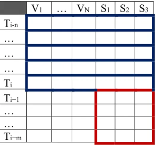
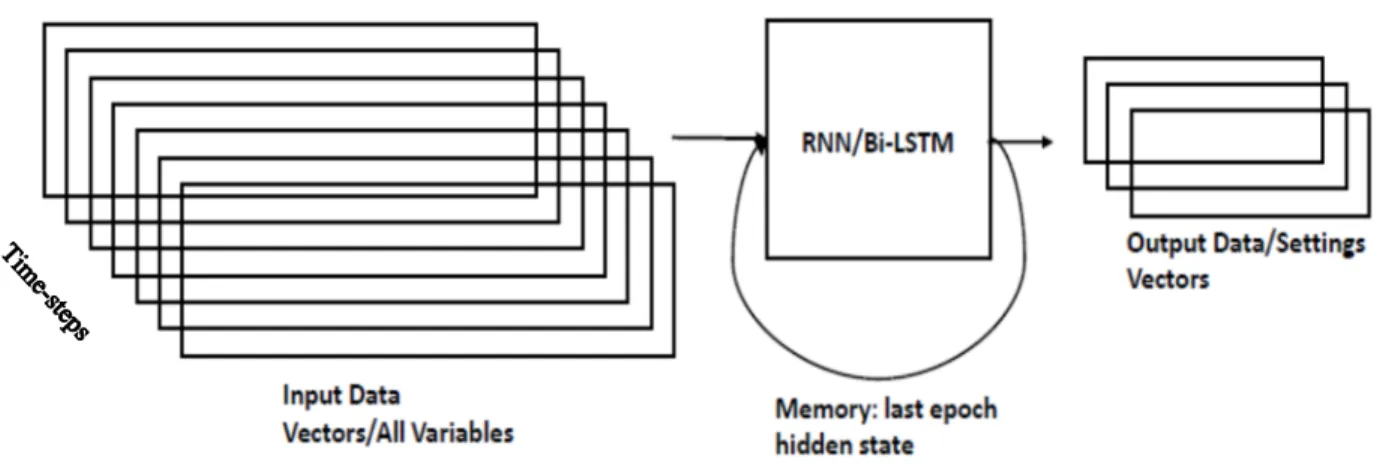
Figure 3.1 Data arrangement for RNN/Bi-LSTM sequence generation for setting variables; prediction of m time-steps for setting variables, given n past time-steps of all input variables, which include the setting variables………..44

Figure 3.2 Sliding window for RNN/Bi-LSTM training, shown for 3 epochs…………..45

Figure 3.3 Prediction of a sequence of m data points by RNN/Bi-LSTM given data point at time-step Ti and its n past data points………45

LIST OF SYMBOLS

δ Random number in [0,1] used for creation of data points by SMOTE algorithm X A given feature vector

xi Data point (observation) of row i of a feature vector X in dataset

xknn Nearest neighbor of data point xi chosen during creation of synthetic data by

SMOTE algorithm

𝑥 Synthetic data created by SMOTE algorithm

x

x

µ Mean of a data distribution within a feature vector

σ Standard deviation of a data distribution within a feature vector

E

W

yi Output of a classifier for observation i

ri Target value for observation i

T Training set

{𝑻𝒊_{} Replicate training sub-sets bootstrapped from training set T} Ƙ Cohen`s Kappa statistic

po Relative observed agreement among raters

pe Hypothetical probability of chance agreement between two raters

n Number of classes N Number of instances

nki Number of times rater i predicted class label k

LIST OF ALGORITHMS

Page Algorithm 2.1 k-fold cross-validation ……….27

LIST OF ABBREVIATIONS SpO2 oxygen saturation

FiO2 oxygen inspired fraction CO2

PEEP

Carbon Dioxide

Positive End-Expiratory Pressure PaO2 Arterial pressure in oxygen PIP Positive Inspiratory Pressure CDSS Clinical Decision Support System AI Artificial Intelligence

PICU Pediatric Intensive Care Unit ANN Artificial Neural Network MLP Multi-Layer Perceptron

ARDS Acute Respiratory Distress Syndrome CDSS Clinical Decision Support System

Bagging Bootstrap Aggregating

SMOTE Synthetic Minority Oversampling Technique EtPCO2 End tidal Partial pressure in CO2

LSE Least Square Error

SGD Stochastic Gradient Descent SVM Support Vector Machine RNN Recurrent Neural Network

INTRODUCTION

Mechanical ventilation assists or controls the inhalation of oxygen into the lungs and the exhalation of carbon dioxide. Many variables need to be monitored during mechanical ventilation. Some of these variables are: expiratory minute volume, expiratory tidal volume, mean airway pressure, peak airway pressure, measured frequency, level of dyspnea, respiratory rate, heart rate, blood pressure, patient-ventilator synchrony, arterial blood gas, oxygen saturation. One of the important variables that the clinician wishes to monitor and control during mechanical ventilation, to ensure it remains within an acceptable range, is the oxygen saturation (SpO2). The SpO2 variable should ideally be maintained between 92% and 97%, at all time, during mechanical ventilation. One of the ways to control the SpO2 is by tweaking some setting variables during mechanical ventilation. The setting variables that we considered in this study, are: oxygen concentration (FiO2) setting, Positive End-Expiratory Pressure (PEEP) setting and Tidal Volume setting. One of the challenges the clinician faces when it comes to monitoring and controlling the SpO2 variable, is being able to forecast the effect that a change in one or more setting variable(s) will have on the SpO2. Although the time for stabilization of SpO2 following a setting change depends on the changes in setting variables, the SpO2 is considered to reach steady state five (5) minutes after the setting change is made. Hence, given the values of measured variables, the setting variables, as well as any change(s) in the values of one or more setting variable(s), at a given time step during mechanical ventilation, the clinician would want to be able to predict the value of SpO2, within a range of acceptable precision, five (5) minutes after the setting change(s) is/are made. At any given time during mechanical ventilation, the clinician may need to decide, based on various respiratory variables, the values by which to tweak the setting variables. These modifications in one or more of the setting variable(s) are intended to allow the SpO2 variable to remain within its acceptable range (92-97%).

In the aim of developing a Clinical Decision Support System (CDSS) for the management of mechanical ventilation, we attempted to create a system that predicts SpO2 when a modification in mechanical ventilation settings is performed. Therefore, the motivation of this research

2

project is to propose a method which is intended to support the clinician in her/his decision-making process when it comes to the settings of FiO2, PEEP and PIP/Tidal Volume variables. This is achieved via the use of a machine learning model (classifier) capable of successfully predicting values of SpO2 based on values of other biological signals, combined with any changes in setting variables made by the clinician. The predictive model used would ideally make it possible for the clinician to have an accurate prediction of the effect any change in the setting variables would have on the SpO2, five minutes after the change is made. As revealed in the previous paragraph, this five-minute duration was prescribed by the clinician as the minimal SpO2 settling time, following a setting change.

The mechanical ventilation expert cannot reasonably be expected to always be present at the patient’s bedside. The development of artificial intelligence (AI) in medicine provides caregivers with assistance in the management of mechanical ventilation variables. The use of AI is intended to improve patient management in intensive care, as well as mechanical ventilation teaching to respiratory therapists and physicians. Several expert systems have been developed based on medical knowledge to help clinicians in the management of mechanical ventilation. However, only a few of them are commercialized and none have been widely in use in intensive care. Another approach is to model patient reaction to mechanical ventilation settings modifications to predict its impact on oxygenation and on CO2 removal, using physiological algorithms rather than supervised learning algorithms. Some physiological algorithms have been developed, but none has been validated for this indication. In the aim of developing a CDSS for the management of mechanical ventilation, we propose a method through which the SpO2 variable can be classified within a predefined set of class labels, when any modification in mechanical ventilation settings is performed. The method we propose is based on machine learning algorithms to develop predictive models via the extraction of patterns from large amounts of available data.

To ensure the feasibility of this study, a large amount of data was required. Therefore, the data for 610 patients were extracted from the CHU Sainte-Justine research database, as per inclusion

3

criteria specified by the clinician. The CHU Sainte-Justine research database contains mechanical ventilation data that were collected over a period of over 2 years. The data of all children (age under 18) admitted to the Pediatric Intensive Care Unit (PICU) of Sainte-Justine Hospital that were mechanically ventilated with an endotracheal tube (invasive ventilation) between May 2015 and April 2017 were included. Exclusion criteria were 2 or more vasoactive drugs (epinephrine, norepinephrine, dopamine or vasopressin) at the same time or an uncorrected cyanotic heart disease (defined by SpO2 always below 97% during PICU stay). For each included patient, the vital signs and ventilatory data, collected every 5 and 30 seconds during PICU stay, were extracted from the CHU Sainte-Justine research database. The main elements of this study were: formatting and pre-processing the raw data obtained from the research database, training a machine learning predictive model through supervised learning, ie., using target variable class labels on a subset of the pre-processed data, and then using the trained model to make predictions on the values of SpO2 five minutes after any setting change is performed by the clinician, on new data (test set). In summary, once the data are pre-processed, the machine learning model is trained and fitted on a portion of the data (the training set) and then tested on new data (test set).

Among the multiple classifiers we tested in throughout the study, the ones which yielded the most satisfactory classification performances were the Artificial Neural Network (ANN), also referred to as Multi-Layer Perceptron (MLP), and the Bootstrap Aggregation (short: “Bagging”) ensemble method applied to complex trees (will be referred to as complex tree “Bagging” or “Bagged” trees). The ability of the model to accurately represent data on which it has never been trained (generalization capability) is evaluated using the following metrics: confusion matrices, precision-recall (for classification precision of the different classes involved), f1-score, and the Cohen’s Kappa statistic.

This study was made up of three (3) main phases: data extraction and pre-processing, training and testing of machine learning classifiers using the available training and testing data, evaluation and comparison of the classifiers based on the classification results they yielded. In the data pre-processing phase, a major task consisted in formatting the data to prepare it to be

4

used for classifier supervised training and testing. Once the data was formatted and cleaned up with the aim of being used for machine learning supervised training, all nineteen of the input variables (or features) which represent the respiratory signals, including the three setting signals, were normalized to values in the range [0, 1]. This was deemed necessary due to the high variability in the value ranges of the input variables. The pre-processing phase also included the definition as well as the data balancing. The necessity to attempt data balancing was made evident by the unsatisfactory results that were obtained, after a few training/testing cycles using a few different supervised learning models, including the ANN and the Ensemble of Bagged Complex Trees. The severe imbalance in the data is caused by the fact that more than 90% of the observations belonged to class-label “3”. This imbalance in the data causes significant bias in the learning of the various class labels by the classifier. This means that a high classification accuracy would not necessarily be representative of the classification accuracy of any of the various class-labels. In simple terms, with such a high degree of data imbalance, the classifier can learn the majority class very well, but doesn’t get enough samples of the other class-labels (minority classes) to be able to learn them well enough. The data balancing process used in this study, consisted in combinations of down-sampling and up-sampling techniques. A down-up-sampling of the majority class and an over-up-sampling using the Synthetic Minority Oversampling Technique, (SMOTE) of the minority classes were needed to balance the three (3) classes of the data involved.

The aim of this study was to find a way to use machine learning models, through supervised learning, to extract knowledge from research data to predict the effect any setting change made by the clinician would have on the SpO2 signal five minutes later.

Some significant contributions were made throughout this research project, namely:

• Large amounts of data from an ICU research database were exploited for SpO2 prediction via machine learning classification models, which, as per the literature reviewed, doesn’t seem to have been done up to this date.

5

• To render the available ventilatory data compatible with machine learning supervised training methods, a data formatting process was proposed.

• To counter the imbalanced nature of the data, various combinations of different data balancing techniques were proposed.

• Supervised machine learning algorithms were proposed for attempting to extract knowledge from large amounts of patient mechanical ventilation data in the aim of predicting the behavior of SpO2, based on values of other variables and those of any setting changes made by the clinician.

CHAPTER 1

LITERATURE REVIEW

The development of machine learning algorithms in the field of AI presents countless promises to the medical field. A medical intervention during which data can be stored about the evolution of the intervention and of the patient’s state, offers the possibility of the integration of machine learning algorithms which could assist the clinician(s) involved in the decision-making process throughout the intervention. The ICU mechanical ventilation is an area, among possibly many other areas of the medical field, to which AI could potentially contribute remarkable progress. However, based on the available information which we have reviewed from research papers, no study which addresses the possibility of SpO2 prediction via machine learning has been undertaken by any research group, yet. Nonetheless, the following section presents a literature review, which includes a study in which an expert system was developed to assist in the mechanical ventilation weaning process. It also presents a review of studies that address topics regarding some data balancing methods used in this study, in the data pre-processing phase. The general conclusion section provides a review of the study by summarizing the essential elements of it and the results it yielded, as well as some recommendations for future work.

8

• Physiologic Cardiorespiratory Simulators, which can reproduce cardiorespiratory physiology and provide arterial blood gas values. An example is the MacPuf simulator developed by C.J Dickinson, 1977. The Dickinson model considers blood circulation, the gas exchange system, ventilation control, and tissue metabolism. It simulates gas exchange and respiratory mechanics according to the alveolar ventilation and gas-exchange time, as well as in terms of respiratory rate, compliance, lung capacity, and oxygen saturation. It requires the setting of 26 parameters to simulate the evolution of the state of the targeted sub-parts of the respiratory system. Another simulator is known as VentSim [22]. It includes a ventilator component, ie., a volume-cycled, constant-flow ventilator, an airway component, and a circulation component. This simulator includes arterial and venous blood gases. It has been validated on simulated patients and showed a good match between the blood gas it provided and that of clinical range. However, a comparative assessment with data from actual ventilated patients is missing, and the ability to simulate unstable patients, which are frequently encountered in ICU’s has not sufficiently been evaluated. SOPAVent [23] developed a simulator based on a 3-compartment physiological model. A significant limitation of this model is that it presently only works with stable patients, which is not a realistic expectation given the reality of ICU’s.

• Simulators for Ventilation Management Recommendations: A model that includes oxygen and carbon dioxide gas exchange and storage modelling and a linear model of lung mechanics, has been developed by Intelligent Ventilator: Rees et al. [19]. The model uses a decision theory approach for lung mechanics simulation. It is combined with penalty functions which allow it to line up with clinical preferences, given the goals and side effects of lung mechanics.

The above-mentioned models all share the limitation of not being suited to learn from ever-growing sets of clinical research data, and potentially improve their simulation performances. This is a major reason for which a machine learning approach to the

9

problem of lung mechanics modeling should be given much attention, as it could prove to be a means by which a CDSS could be rendered reliable enough to provide significant support to ICU physicians. In this study, we propose a method for predicting SpO2 via a supervised machine learning algorithm, using patient data which we extracted from CHU Ste-Justine Hospital research database.

CHAPTER 2

USING MACHINE LEARNING MODELS TO PREDICT OXYGEN SATURATION FOLLOWING VENTILATOR SUPPORT ADJUSTMENT IN CRITICALLY ILL

CHILDREN: A SINGLE CENTER PILOT STUDY

ABSTRACT

Clinical experts in mechanical ventilation are not continuously at each patient’s bedside in an intensive care unit to adjust mechanical ventilation settings and to analyze the impact of ventilator settings adjustments on gas exchange. The development of clinical decision support systems analyzing patients’ data in real time offers an opportunity to fill this gap. The objective of this study was to determine whether a machine learning predictive model could be trained on a set of clinical data and used to predict hemoglobin oxygen saturation 5 min after a ventilator setting change. Data of mechanically ventilated children admitted between May 2015 and April 2017 were included and extracted from a high-resolution research database. More than 7.105 _{rows of data were obtained from 610 patients, discretized into 3 class labels.} Due to data imbalance, four different data balancing process were applied and two machine learning models (artificial neural network and Bootstrap aggregation of complex decision trees) were trained and tested on these four different balanced datasets. The best model predicted SpO2 with accuracies of 76%, 62% and 96% for the SpO2 class “< 84%”, “85 to 91%” and “> 92%”, respectively. This pilot study using machine learning predictive model resulted in an algorithm with good accuracy. To obtain a robust algorithm, more data are needed, suggesting the need of multicenter pediatric intensive care high resolution databases.

Sam Ghazal1_{, Michael Sauthier MD}2_{, David Brossier MD}2_{, Wassim Bouachir PhD}3_{, Philippe Jouvet MD PhD}2_{, Rita Noumeir PhD}1 1_{Laboratoire de traitement de l'information en santé (LATIS) - École de Technologie Supérieure (ÉTS),} 2_{Centre Hospitalier Universitaire Sainte-Justine (CHUSJ),} 3_{LICEF research center - TÉLUQ University}

Research paper published: Ghazal S, Sauthier M, Brossier D, Bouachir W, Jouvet PA, Noumeir R; Using machine learning models to predict oxygen saturation following ventilator

support adjustment in critically ill children: A single center pilot study: PLoS ONE 14(2):

12

2.1 Introduction

In case of respiratory failure, mechanical ventilation supports the oxygen (O2) diffusion into the lungs and the carbon dioxide (CO2) body removal. As an expert in mechanical ventilation cannot reasonably be expected to be continuously present at the patient’s bedside, specific medical devices aimed to help in ventilator settings adjustments may help to improve the quality of care. Such devices are developed using either algorithms based on respiratory physiology/medical knowledge that adapt ventilator settings in real time based on patients’ characteristics but are not accurate enough to be used widely in clinical practice, especially in children [1, 2]; or physiologic models that simulate cardiorespiratory responses to mechanical ventilation settings modifications but none was validated for this indication [3]. The above-mentioned models all share the limitation of not being suited to learn from ever-growing sets of clinical research data, and potentially improve their performances. To overcome this drawback, another avenue is the development of algorithms using artificial Intelligence to provide caregivers with support in their decision-making tasks. In this study, we assessed machine learning methods to predict transcutaneous hemoglobin saturation oxygen (SpO2) of mechanically ventilated children after a ventilator setting change using a high-resolution research database.

13

2.2 Materials and Methods

This study was conducted at Sainte-Justine Hospital and included the data collected prospectively between May 2015 and April 2017 of all the children, age under 18 years old, admitted to the Pediatric Intensive Care Unit (PICU) who were mechanically ventilated with an endotracheal tube. Patients’ data were excluded if the patient was hemodynamically unstable defined as 2 or more vasoactive drugs delivered at the same time (ie., epinephrine, norepinephrine, dopamine or vasopressin) or with an uncorrected cyanotic heart disease defined by no SpO2 > 97% during all PICU stay. All the respiratory data from included patients were extracted from the PICU research database [4], after study approval by the ethical review board of Sainte-Justine hospital (number 2017 1480).

14

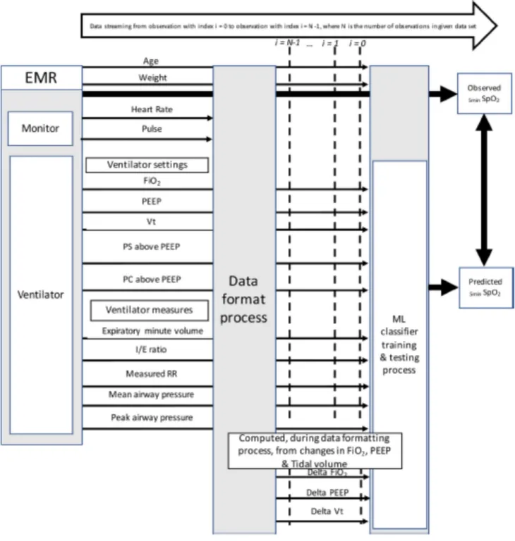
Figure 2.1 Schematic description of the analysis process and items involved

EMR: electronic Medical Record, FiO2: inspired fraction of Oxygen, Vt: tidal volume, PEEP: Positive end expiratory pressure, PS above PEEP: pressure support level Above PEEP, PC above PEEP: pressure control level above PEEP, MVe: expiratory minute volume, I:E Ratio: inspiratory time over expiratory time, Measured RR: respiratory rate measured by the ventilator, PIP: positive inspiratory pressure ie maximal pressure measured during inspiration. 5 m i nSpO2: SpO2 observed 5 min after PEEP, FiO2, tidal volume, PS above PEEP, PC above PEEP change, ML: machine learning, ANN: artificial neural network, BACDT: Bootstrap aggregation complex decision trees.

15

2.3 Methodology 2.3.1 Data extraction

To determine the data that will be extracted for each child, an item generation was conducted by three physicians (PJ, MS, DB). The resulting items are presented in Fig 2.1 within their sources, means of extraction and a schematic of the main components of the study. The predictive SpO2 value was the SpO2 5 minutes after a change of a ventilator setting. The delay of 5 min corresponded to the shortest period of time to reach a steady state after modification of a ventilator setting [5].

2.3.2 Data Categorization

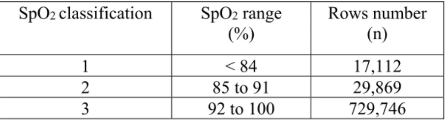
SpO2 levels at 5min were classified into three categories (Table 2.1). The thresholds were selected according to clinical value: a SpO2 < 92% is a target to increase oxygenation in mechanically ventilated children [6]. The critical level of 85% SpO2 is used as an alarm of severe hypoxemia in intensive care [7].

16

The SpO2 variable (target) has been classified in three categories to correspond to clinically relevant values.

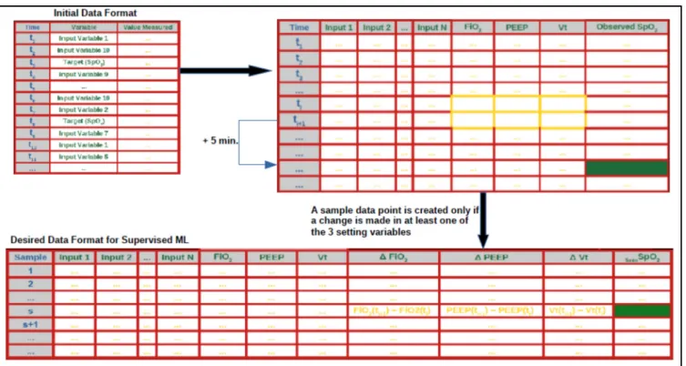
2.3.3 Data formatting

The extraction of data from the patient database produces data files with a format which does not allow for classifier training. This is mainly because, in these initial data files, the respiratory variables are not separated in columns, which would become the input and output vectors during model training. Moreover, a significant proportion of rows in the initial files do not represent data which are measured within mechanical ventilation time intervals. Thus, it is necessary for the formatted files which are to be used for classifier training to be rid of any unnecessary rows, which do not contain mechanical ventilation readings.

The classifiers used to predict (classify) the SpO2 values are built when mathematical models are trained on a set of data which displays the relevant variables in a table format. The table must be arranged as follows: the respiratory signals (variables) represent the labels of the various columns and the data storing times and patient codes represent the rows. The data formatting process described herein consists basically in making the data format machine learning friendly. Below are the steps taken to format and pre-process the raw data to make it suitable for classifier training. Many of the data pre-processing criteria have been established by the clinicians involved in this study.

• Read content of initial data file into a Python (Pandas library) data frame: The data contained in the initial files are stored into data frames which are used to manipulate and preprocess the data.

Table 2.1: Definition of SpO2 class labels specifications SpO2 classification SpO2 range

(%) Rows number (n)

1 < 84 17,112

2 85 to 91 29,869

17

• Strip away the microseconds part from the data storing times in the initial files, as it is not contextually relevant: Following this step, the storing times are represented in the following form: “year:month:day:hours:minutes:seconds”

• Pivot the data that were stored in the data frames: This step transforms the data from the linear format in the initial files into a table, where the biological variables are the column labels and the patient codes and storing times are the row labels.

• Align the data of the variables in the pivoted table within mechanical ventilation time slots: Since the readings for the various variables involved are not all set at the same frequency, the data for the different variables are not aligned along the rows (time-steps). Therefore, it is necessary to align the data readings for the various variables (along any given row within a mechanical ventilation interval), to prepare the data to be used for classifier training. This data formatting step ensures the alignment of the data for “FC”, “SpO2”, “Pulse”, "Pressure Support Level Above PEEP" and "Pressure Control Level Above PEEP" variables with the data of the other variables, for any given time-step within mechanical ventilation time-slots.

• Fill cells of “Tidal Volume Setting” variable with the values given by “Expiratory Minute Volume” / “Measured Frequency” x 1000, as per clinician`s requirement. • Drop rows with any empty cell(s): Once alignment of the data is completed, all rows

containing empty readings are to be dropped to ensure that only time-slots of mechanical ventilation readings are preserved.

• Create 3 new variables which represent the changes made to the setting variables (one for each setting variable): Run through all the rows in the data frame, and for any of the 3 setting variables (FiO2, PEEP, Tidal Volume), if the value at any time-step is NOT EQUAL to the value at the previous time-step, then calculate the difference between the values at both time-steps and place the results in new columns, called “Delta FiO2 Setting”, “Delta PEEP Setting” and “Delta Tidal Volume Setting”. This step allows the creation of three (3) new variables: “Delta FiO2 Setting”, “Delta PEEP Setting” and “Delta Tidal Volume Setting” which are deemed very significant for the prediction of SpO2 (5 min. following the change in at least one of the setting variables). For each patient section (as per the patient code), whenever the readings show that at least one of the three (3) setting variables (FiO2, PEEP, Tidal Volume) is modified from one row (time-step) to the next,

18

the values of the differences are stored in the new columns created (“Delta FiO2 Setting”, “Delta PEEP Setting” and “Delta Tidal Volume Setting”). This means that only the time-steps at which at least one of the setting variables is modified are to be preserved in the data file to be used for classifier training.

There are two main conditions for this step:

1) To verify that the data of different patients are treated separately, as per the patient codes which these data are grouped by. This ensures that the readings for different patients are not mixed up. In other words, the various sections of rows which are grouped by the patient codes are to be treated separately.

2) To verify that the change in “FiO2 Setting” does not exceed 20%, as per clinician’s requirement.

Copy the value of “SpO2” at the row 5 minutes following the current examined row, into the current row, in a column assigned to this variable: “SpO2 in 5 min.”.

• Create a new column called “Binned SpO2” in the data frame and fill it with values

as per the binning criteria in table 1. This variable is to be used as the target variable: The target variable is created by binning the data of variable “SpO2 in 5 min.” into three classes (see table 2.1). The binning of the target variable data into three classes allows for better classification performance, since it reduces the size of the range of values that the trained model would have to predict from. This naturally implies that it increases the amount of observations per target class label, which allows the classification model to extract more information per class label, during the training process.

• For all time-steps, verify the accuracy of “FC” readings by making sure that they are within ± 10 of “Pulse”: All rows containing “FC” readings which do not respect this condition are dropped.

19

• Add “Age” and “Weight” data of all patients to the data frame: Using the Patient-specific data file and the data frame which represents the data file which is used to train the predictive model, the age and the weight of every patient are added to the data frame in which the data is being formatted. The weight and the age of each patient, at the time of undergoing mechanical ventilation, are inserted in their newly created columns, at the appropriate rows, in the data frame. The data frame containing the formatted data is copied into a comma-separated file (csv) file.

20

Figure 2.2 presents a visual overview of how we performed cleaning and formatting of the data to prepare it for supervised learning.

2.3.4 Feature standardizing and scaling

The predictive model’s training/testing trials have been carried out both on standardized and on scaled input data. These data pre-processing steps were deemed necessary, since the input variables have ranges of values which are very dissimilar.

21

The standardization (z-score normalization) transforms the various data vectors (variables) in such a way that they’ll have the properties of a standard normal distribution with µ = 0 and σ = 1. Standardizing the variables so that they are centered around zero with a standard deviation of 1 is not only important when measurements that have different units are compared, but it is also a general requirement for many machine-learning algorithms, including ANNs. The standardization is performed (ie., the z-score is computed) for every observation xi of a variable

X, using the mean µ(𝑿) of the variable and its standard deviation 𝜎(𝑿).

The data rescaling, on the other, allows for the conversion of the different input variable ranges to a common range, namely [0,1]. Feature data rescaling is performed as follows:

𝑥 =

In equation 2.1,

x

x

maximum values of feature X, respectively.

For the data involved in this study, feature rescaling yielded better results than feature standardizing on model training and testing performances. Therefore, all the results presented in this paper are the ones obtained via training and testing of the classifiers on the rescaled data (eq. 2.1).

2.3.5 Data Balancing

The data analysis showed a severe imbalance with most SpO2 at 5min above 92%. This is logical as caregivers want to maintain SpO2 in normal range during child PICU stay. In such condition, the classifier learns the majority class label (class 3) (Table 2.1) but doesn’t learn the minority class labels (classes 1 and 2) [8]. The data balancing process aims to allow the classifier to learn from all class equally. The data balancing process used in this study included a combination of down-sampling and up-sampling techniques: to balance the three classes of the data involved, a down-sampling of the SpO2 class 3 using TOMEK algorithm [9] and an

22

over-sampling of SpO2 class 1 and 2 using Synthetic Minority Oversampling Technique (SMOTE) [10] were performed.

The very imbalanced nature of the studied data presented a significant challenge. A data balancing process was required prior to training and classification. As previously mentioned, the range of values of the target variable is binned into three class labels (table 2.1). The severe imbalance in the data is caused by the fact that most observations belonged to the class labelled “3”, since most SpO2 readings happen to be 92% or above. This imbalance in the data causes significant bias in the learning of the various class labels by the classifier. This means that a high classification accuracy would not necessarily be representative of the classification accuracy of any of the various class labels. In simple terms, with such a high degree of data imbalance, the classifier can learn the majority class very well. However, it doesn’t get enough samples of the minority class labels to be able to learn them well enough. The data balancing process used in this study included a combination of down-sampling and up-sampling techniques. To balance the three classes of the data involved, a down-sampling of the majority class and an over-sampling of the minority classes were performed.

The down-sampling process was made up of the following steps:

1) TOMEK algorithm used to detect TOMEK links throughout the whole dataset, for all three classes, and remove them. TOMEK links are the links between any two observations considered nearest neighbors, but which belong to different classes, ie., have different class- labels [17]

2) Remainder of points to be removed are selected at random.

The oversampling process consisted of using the Synthetic Minority Oversampling Technique (SMOTE). The SMOTE algorithm, as its name indicates, creates synthetic points between a point and its nearest neighbors (the number of nearest neighbors used for each observation depends on the proportion by which the cardinality of the minority class is to be increased). These synthetic points replace the original points (observations) that belonged to the minority class being oversampled. The fact that the points created by SMOTE are synthetic does not

23

necessarily hinder the generalization capability of the classifier, because all the synthetic points are placed between the original observation and a number k of its nearest neighbors [10]. The creation of synthetic data points by SMOTE can be formulated as follows:

In equation (2.2),

x

x

neighbors, and δ is a random number in [0,1] which determines the position of the created synthetic data point along a straight line joining the original data point xiand its chosen nearest

neighbor xknn.

Sections 2.3.6 presents the two mathematical models that have yielded the most satisfying results in SpO2 value predictions, five minutes following any change in at least one of the setting variables.

2.3.6 SpO2 Classification

To identify the best machine learning classification method, we tested various classification models on the four balanced datasets, of which the two (2) that yielded the best results were considered: artificial neural network and bagged complex decision trees.

2.3.6.1 Artificial Neural Network (ANN) Training and Testing

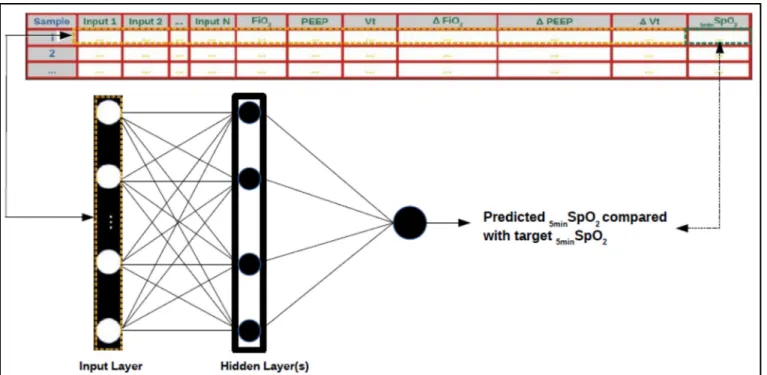
Once the data has been formatted and pre-processed, a machine learning predictive model can be trained on a sub-set of labeled training data. The model is then used to predict the target variable values on a testing subset where the class labels are hidden. We used Artificial Neural Networks (ANN) to make predictions of the SpO2 variable, based on the values of other variables of interest. The values of the three setting variables and the changes applied to them were also used by the model as predictor variables. Through the function approximation that the ANN performs, it is possible to make predictions of SpO2 variable, based on the input data.

24

For SpO2 classification categories, please refer to table 2.1.

The ANN is trained on a set of training data, using the backpropagation algorithm, as follows: • It takes in the values of all input variables of interest.

• It tunes its weights and creates a non-linear decision boundary to classify the response. A linear decision boundary is necessary to classify a target variable that varies in a non-linear fashion with respect to its explanatory variables, the input variables. In other terms, a non-linear decision boundary is required when the output cannot be reproduced from a linear combination of the inputs, which is very often the case. An activation function, such as the sigmoid, allows to model this nonlinear relationship between the input variables and the target variable. Without an activation function, an ANN only provides a linear transformation, ie., the outputs of a layer multiplied by the weights of their connections with the next layer [3].

• The output (SpO2) is predicted based on the series of linear transformations followed by the creation of a non-linear decision boundary via the combinations of these transformations with the activation function(s) used.

The learning algorithm runs through all the rows of data in the training data set and compares the predicted outputs with the target outputs found in the training data set. • The weights are adjusted via supervised learning, in a manner to minimize the error of

predicted SpO2 vs target SpO2.

• The process is repeated until the error is minimized.

The training of the ANN is carried out using a portion of the data available (ie., a training set). Once the training is completed, the model is tested on a test set, which is the data that was excluded during the training phase. The test set serves to validate the generalization of the model, meaning its ability to accurately predict output data based on new input data. The results obtained by this method of training/testing are presented in table 2.2.

The ANN classifier was implemented through cycles of forward propagation followed by backward propagation through the network’s layers. The backpropagation algorithm is used

25

for performance optimization. It fine-tunes the weights which, initially, are randomly set, so that the error function is minimized. The error function computes the difference between the ANN’s output and its expected output, after an input example has been propagated through it. For instance, when the normalized data is presented to the ANN, the 18 inputs whose values are in [0, 1] are presented to the ANN, through the input units. These values, along with a bias value inserted into the ANN as input, are processed through the units with the sigmoid activation function, making up the middle layers of the ANN. Then, an output is produced representing the estimation, or prediction in the set {“1”, “2”, “3”}, of the SpO2 value five minutes after the change in settings. The weights of the ANN are modified at each run through the training data, in the aim of minimizing the classification error. The loss function used for classification by the MLP is cross-entropy.

For a given number of classes K > 2, the cross-entropy error can be formulated as shown in eq. 2.3, where {Wi}i is the matrix of weights between the neuron layers, ri is the target value. yi is

the value generated by the ANN, ie., its output.

E

( W

|

𝑥 , 𝑟 ) = - ∑ 𝑟 𝑙𝑜𝑔 𝑦

The outputs of the ANN are:

𝑦 =

Using stochastic gradient-descent (SGD) for error minimization, the update rule for the ANN weights, is:

∆

𝑤 = 𝑛(𝑟 − 𝑦 )𝑥

In equation 2.5, η is the learning rate which, when SGD is used, decreases as the error is minimized. During ANN training, each observation, comprised of an input vector and a target output, is denoted (xt_{, r}t_{), with r}t _{ϵ {“1”, “2”, “3”}. The reason why the cross-entropy (eq. 2.3)}

26

is used instead of the Least Square Error (LSE) is to avoid long periods of training, due to the ANN going through stages of slow error reduction, ie., SGD local minima. The MLP classifiers were implemented with the use of the Scikit-Learn package within the Python programming language [http://scikit-learn.org].

Figure 2.3 Schematic representation of ANN supervised training

2.3.6.2 Bootstrap Aggregation of complex decision trees training and testing

Bootstrap aggregating (acronym: bagging) was proposed by Leo Breiman in 1994 to improve classification by combining classifications of randomly generated training sets [8]. “Bagging” allows for the creation of an aggregated predictor via the use of multiple training sub-sets taken from the same training set, hence the term “bootstrapping”. In other words, multiple versions of a predictor are created through the bootstrapping of the various training subsets. This aggregation of predictors generally allows for more accurate predictions (or classifications) than can be obtained through a single predictor. Thus, it can be considered as a wonderful technique used for improving a classifier’s performance. It is noteworthy to mention that this method (bootstrap aggregation or “bagging”) doesn’t always improve the given classifier’s performance, but it does most of the time.

27

Let {𝑻𝒊_{} denote the replicate training sub-sets bootstrapped from the training set T. These} replicate sub-sets each contain N observations, drawn at random and with replacement from T. For each of these sub-sets of N observations, a prediction model (classifier) is created. The computational model used for “bagging” was “complex decision trees”. This means that, for each bootstrapped sub-set of training data, a complex decision tree is trained and thus a classifier is created. If i = 1, …, n, then n classifiers are created through the “bagging” process.

A decision tree is a flowchart computational model which can be used for both regression and classification problems. Paths from the root of the tree to its various leaf nodes go through decision nodes in which decision rules are applied in a recursive manner, based on values of input variables. Each path represents an observation (X, y) = (x1, x2, x3, …, xn, y), where the

label assigned to the target y is given in the leaf node, at the end of the path (ie., classification).

In the aim of maximizing the model’s generalization capability during the training process, the Bagged Complex Trees’ performance is tested via k-fold cross-validation. A value k = 10, which is common practice, was used in this study. The training using k-fold cross-validation is carried out as described in algorithm 2.1:

Algorithm 2.1 k-fold cross-validation

• The data set is first divided into two parts; the training-set and the test-set. • The training of the “Bagged” Complex Trees includes a k-fold cross-validation,

which is performed as follows:

 Randomly partition the data-set into k equal-sized subsets (folds).  For each of the k equal-sized subsets:

 Train/fit the model on the elements contained in the other (k-1) subsets.  Test the model’s accuracy on the given subset.

 Iterate over the k subsets, until each one has been used once for testing the model’s performance during its training.

 The training validation score consists of the average score obtained by validating the model on all k subsets.

28

The mathworks Matlab R2016b Machine Learning toolbox was used for the creation of the ensemble of “Bagged” complex trees model.

2.4 Assessment of performances of classifiers

We evaluated the performances of the classifiers based on the metrics including testing confusion matrix, average accuracy, precision, recall and F score [14] with a 5minSpO2 prediction expected above 0.9 for each class.

• Test confusion matrix :

In a confusion matrix, the diagonal made up of the intersections of target and predicted SpO2 is where the rates of correct classifications are provided.

• Cohen’s Kappa (eq. 2.6)

Ƙ =

In labeling problems involving a number of class-labels n > 2, it is generally appropriate to estimate the agreement between the classifier and ground truth using a statistic known as Cohen’s Kappa (κ), which is in [0, 1], with 1 being perfect agreement and 0, no agreement whatsoever b. In equation 2.6, po is the observed agreement and pe (eq. 2.7) is the hypothetical

probability of agreement by chance, based on the distribution of the data among the n classes. In other words, pe is the agreement expected by chance. In equation 2.7, N is the number of

observations, with nk1 as the number of times class-label k appears in ground truth, and nk2 as

the number of times the classifier predicted class-label k, with k = 1,…,n .

𝑝 =

∑

𝑛 𝑛

29

𝐴𝑐𝑐𝑢𝑟𝑎𝑐𝑦 =

• Precision (eq. 2.9):

𝑃𝑟𝑒𝑐𝑖𝑠𝑖𝑜𝑛 =

The Precision (eq. 2.9) is the ratio of all correct classifications for class i to all instances labeled as class label i by the model. In a non-normalized confusion matrix, this would mean dividing the number of instances classified in class label i by the total of instances in column i.

• Recall (eq. 2.10):

𝑅𝑒𝑐𝑎𝑙𝑙 =

Recall (eq. 2.10) is the ratio of the number of instances classified in class label i to the number of true class i labels. Again, in a non-normalized matrix, this would require dividing the number of instances classified in class label i by the total of row i.

30

F1-score (eq. 2.11) :

𝐹1 − 𝑠𝑐𝑜𝑟𝑒 =

The F1-score (eq. 2.11) provides a single measure of classification performance of the model used. In the case of class-imbalanced datasets, the F1-score is better than the accuracy metric, which is simply the ratio of correctly predicted observations to the total number of observations. Mathematically, it is the harmonic mean H, computed using Precision and Recall (eq. 2.12). In equation 2.12, x1 to xn represent n positive real numbers.

For the F1-score (eq. 2.11), n = 2, x1 and x2 are the values of Precision and Recall.

𝐻 =

∑

, 1 < 𝑖 < 𝑛

The values of these performance metrics for our eight experiments are presented in table 2.2.

31

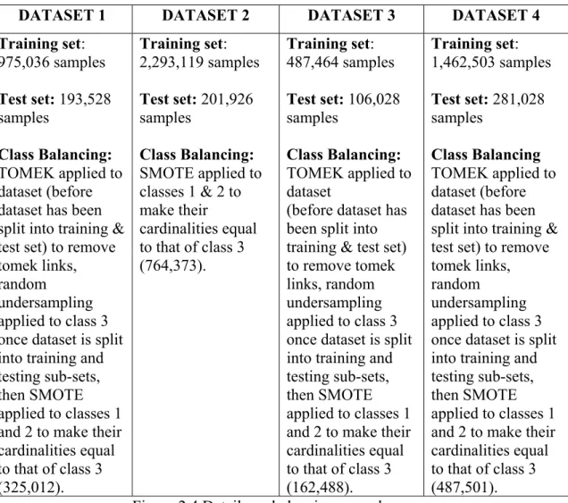
DATASET 1 DATASET 2 DATASET 3 DATASET 4

Training set: 975,036 samples Test set: 193,528 samples Class Balancing: TOMEK applied to dataset (before dataset has been split into training & test set) to remove tomek links, random

undersampling applied to class 3 once dataset is split into training and testing sub-sets, then SMOTE applied to classes 1 and 2 to make their cardinalities equal to that of class 3 (325,012). Training set: 2,293,119 samples Test set: 201,926 samples Class Balancing: SMOTE applied to classes 1 & 2 to make their cardinalities equal to that of class 3 (764,373). Training set: 487,464 samples Test set: 106,028 samples Class Balancing: TOMEK applied to dataset

(before dataset has been split into training & test set) to remove tomek links, random undersampling applied to class 3 once dataset is split into training and testing sub-sets, then SMOTE applied to classes 1 and 2 to make their cardinalities equal to that of class 3 (162,488). Training set: 1,462,503 samples Test set: 281,028 samples Class Balancing TOMEK applied to dataset (before dataset has been split into training & test set) to remove tomek links, random

undersampling applied to class 3 once dataset is split into training and testing sub-sets, then SMOTE applied to classes 1 and 2 to make their cardinalities equal to that of class 3 (487,501). Figure 2.4 Details on balancing procedures

32

Table 2.2 Classification performance metrics results for MLP and bagged tree classifiers

Da ta set (f igure 2. 5) 2. MLP Bagged Trees

precision recall f1-score Cohen’s Kappa precision recall f1-score Cohen’s Kappa

Da ta set 1 Label 1 0.12 0.70 0.21 0.16 0.80 0.76 0.78 0.68 Label 2 0.16 0.43 0.23 0.61 0.56 0.59 Label 3 0.96 0.67 0.79 0.97 0.98 0.97 Avg/total 0.88 0.65 0.73 0.94 0.94 0.94 Da ta set 2 Label 1 0.09 0.72 0.16 0.13 0.77 0.72 0.74 0.66 Label 2 0.09 0.47 0.16 0.57 0.53 0.55 Label 3 0.98 0.70 0.81 0.98 0.99 0.98 Avg/total 0.93 0.69 0.78 0.96 0.97 0.97 Da ta set 3 Label 1 0.16 0.68 0.25 0.20 0.80 0.76 0.78 0.70 Label 2 0.26 0.42 0.33 0.67 0.62 0.65 Label 3 0.92 0.60 0.72 0.95 0.96 0.96 Avg/total 0.80 0.58 0.65 0.91 0.91 0.91 Da ta set 4 Label 1 0.09 0.69 0.16 0.13 0.80 0.74 0.77 0.66 Label 2 0.12 0.47 0.19 0.58 0.54 0.56 Label 3 0.97 0.68 0.80 0.98 0.98 0.98 Avg/total 0.92 0.67 0.76 0.96 0.96 0.96

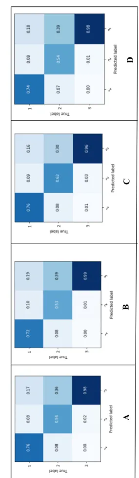
33 Fi g u re 2 .5 MLP test co nfusion matr ices f rom tra inin g/tes tin g (A : datas et 1, B : datase t 2 , C : datase t 3 , D : data se t 4 ) Fig u re 2 .6

Bagged trees test

confusion matr ices from tra inin g/tes ting (A : datase t 1, B : data set 2, C : datase t 3, D : datase t 4 ) A B C D A B C D

34

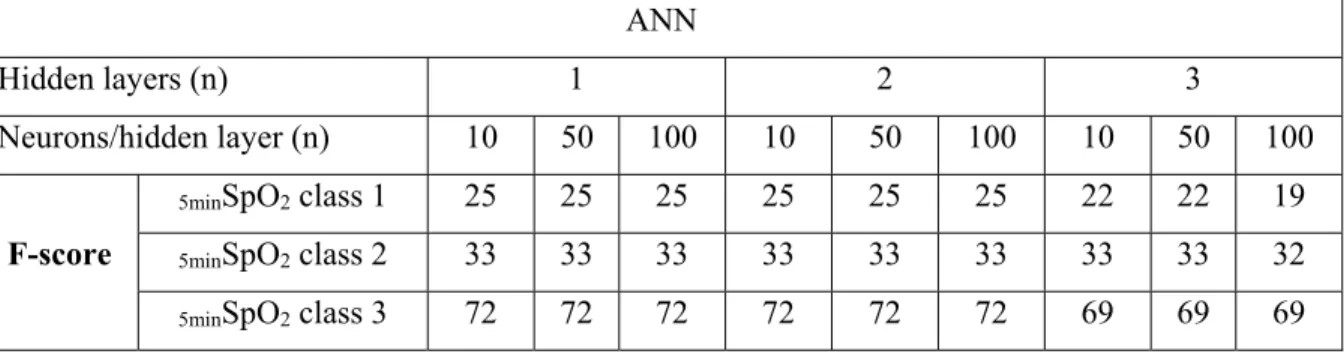
For the ANN, or MLP, the variation of the number of hidden layers and number of neurons per hidden layer did not seem to have a significant effect on the model’s classification performance. As for the Bagged complex trees, the variation of the number of complex trees did not yield significant changes in classification performance. However, the experiments revealed that the data balancing processes had significant influence on SpO2 classification accuracy.

As the classification metrics and the confusion matrices presented in table 2.2 and figures 2.5 and 2.6 reveal, the ensemble of bagged complex trees model has performed significantly better than the ANN. The darker colors in a confusion matrix represent the higher levels of accuracy obtained. According to what has been previously mentioned in the “related work” section regarding Bagging being generally a successful technique for medical data classification [8], it is not surprising that tree Bagging fared better than the other classifiers used in this study. It is noteworthy however to mention that the gaps in performance results between the training and testing confusion matrices are relatively higher in the case of bagged trees model than in that of the MLP. This seems to indicate that, although the bagged trees model was capable of learning very well from the data, there’s still room for improvement in the generalization, especially for class-label “2” data.

The classification performance metrics (table 2.2) show that the bagged trees classifier trained on dataset #3 has yielded the best classification performance on the test sets. The interpretation of the results of this training/testing is provided in the following paragraphs.

In equation 2.6, po is the relative observed agreement among raters, or the ground truth labels

and the classifier’s labels, and pe (eq. 2.7) is the hypothetical probability of chance agreement,

using the observed data to calculate the probabilities of each observer randomly picking each class. If the raters are in complete agreement, then κ = 1. If there is no agreement among the raters other than what would be expected by chance, as given by pe, κ ≈ 0. This would simply

35

for the Cohen’s Kappa statistic was obtained by the bagged trees model trained on training set #3. This is representative of the rate of agreement between the two raters, or between ground truth labels and a machine learning predictive model. In equation 2.7, n is the number of classes, N is the number of instances classified by each rater which, in our case, is ground truth vs classifier, and nki represents the number of times rater i predicted class label k. The

confusion matrix of the ensemble of bagged trees shows that it could correctly classify 76% of class- label “1” data, 62% of class-label “2”, and 96% of class-label “3”. This considerable variation in classification performances of the three class labels can be explained by the huge variation in the numbers of observations available for each of the class labels in the data used in this study. Refer to section A for details on patient sub- population studied.

The SMOTE algorithm is designed in such a way that should theoretically not affect the generalization of the trained model. In cases of extreme data imbalance, however, as is the case in this study, the over-sampling within the data space of a given minority class label, used for increasing the cardinality of the class label’s set, is also likely to be extreme. This may render the data space of this class relatively dense with respect to the rest of the data, made up of real data points of the studied patient sub-population. This may potentially explain the classification model’s relatively poor generalization for class-labels “1” and “2” with respect to the generalization for class-label “3”. Another important consideration to make, in an attempt to explain the hindering effect that the over-sampling seems to have on the generalization of the classifier, is the following: since SMOTE generates synthetic data points by interpolating between existing minority class instances, it can obviously increase the risk of over-fitting when classifying minority class labels, since it may duplicate minority class instances, ie., data points. The fact that the training confusion matrix shows extremely high classification performances for the minority class labels “1” and “2”, as opposed to those shown in the testing confusion matrix, suggests that the over-sampling of the minority class labels using SMOTE could have caused some overfitting for these classes, but this would have to be further investigated.

36

The accuracy (eq. 2.8) of the ensemble of bagged complex trees in classifying SpO2 for dataset #3 is 91%. This metric is very misleading, as it does not consider the imbalance in the numbers of instances of each of the three (3) class labels. This high accuracy (91%) can be, in a considerable part, explained by the fact that class-label “3” makes up 83% of all instances in the testing dataset, and that 96% of class-label “3” data are correctly classified. In other terms, there are 84,171 correct classifications for class-label “3” alone, out of 106,028 observations in the test set. The total number of correct classifications for all 3 class-labels is 96,667 out of a total number of observations of 106,028, ie., an accuracy of 91%. It is thus easy to see why this percentage of correct classifications is not representative of the model’s accuracy in classifying the data of the three (3) classes involved. Clearly, the accuracy metric is not reliable for the evaluation of the performance of our model, hence the importance of the other metrics presented herein.

The F1-score for our model reveals that the model performed very well when predicting class-label “3”. Although the model also performed significantly well for class-class-label “1”, some over-fitting seems to have occurred for classes “1” and “2”, the minority classes, during the training phase. Therefore, some recommendations for improvement in classification accuracy for the minority classes will be provided in the following section.

2.5 Results and Discussion

We developed and assessed the performances of two machine learning classifiers on four different balanced datasets to predict SpO2 at 5 min after a ventilator setting change (ie FiO2, PEEP, Vt/Pressure), in 610 mechanically ventilated children. In Fig 4 and Table 2.2, we report the performances of these two classifiers. Using the classification performance metrics, the bagged trees classifier trained on dataset #3 (see Fig 2.2) has yielded the best classification performance on the test sets (Table 2.2). The confusion matrix of the whole bagged trees shows that SpO2 at 5 min could correctly predict in 76% of class “1” data, 62% of class “2”, and 96% of class “3” (Fig 2.4). This huge variation in classification performances of the three class

37

labels can be explained by the large variation in the numbers of observations available for each of the class-labels in the initial dataset that has limited the machine learning (Table 2.1).

Table 2.3 Absence of impact on performance of the increase of neurons and hidden layers for artificial neural network (ANN). Example of the performance assessed by the F score on the balanced dataset 3 (see fig 2.2)

ANN

Hidden layers (n) 1 2 3

Neurons/hidden layer (n) 10 50 100 10 50 100 10 50 100

F-score

5minSpO2 class 1 25 25 25 25 25 25 22 22 19

5minSpO2 class 2 33 33 33 33 33 33 33 33 32

5minSpO2 class 3 72 72 72 72 72 72 69 69 69

Table 2.4 Absence of impact on performance of the number of complex trees for bootstrap aggregation of complex decision trees (BACDT). Example of the performance assessed by the F score on the balanced dataset 3 (see Fig 2.2)

BACDT

n = 30 n=50

F-score

5minSpO2 class 1 78 78

5minSpO2 class 2 65 65

5minSpO2 class 3 96 96

In agreement with previous studies regarding bagging being a better method for medical data classification, tree Bagging fared better than the artificial neural network used in this study [12]. It is noteworthy however that the gaps in performance results between the training and testing confusion matrices are relatively higher in the case of bagged trees model than in that of the artificial neural network (Fig 2.5). This seems to indicate that, although the bagged trees model was capable of learning very well from the data, there’s still room for improvement in the generalization. The SMOTE algorithm is designed in such a way that should theoretically not affect the generalization of the trained model. In cases of extreme data imbalance, however, as is the case in this study, the over-sampling within the data space of a given

38

minority class label, used for increasing the cardinality of the class label’s set, is also likely to be extreme. This may render the data space of this class relatively dense with respect to the rest of the data, made up of real data points of the studied patient sub-population. This may potentially explain the classification model’s relatively poor generalization for 5minSpO2 class “1” and “2” with respect to the generalization for 5minSpO2 class “3”. Also, since SMOTE generates synthetic data points by interpolating between existing minority class instances, it can obviously increase the risk of over-fitting when classifying minority class labels, since it may duplicate minority class instances. The fact that the training confusion matrix shows extremely high classification performances for the minority 5minSpO2 class “1” and “2”, as opposed to those shown in the testing confusion matrix, suggests that the over-sampling of the minority 5minSpO2 class using SMOTE could have caused some overfitting for these classes, but this would have to be further investigated.

The strengths of this study include a large clinical database of mechanically ventilated children used with more than 7.105 _{rows. In a recent similar study in PICU, 200 patients were included} with 1.15.103 _{rows [15]. However, the volume of data is clearly insufficient. To use such} machine learning predictive models, the pediatric intensive care community needs to combine multicenter high-resolution database. In addition, children data could be pooled to neonatal and adult intensive care data, when possible, such as MIMIC III database [16]. The other strength is the process used to transform the data into a usable format and to correct a variety of artifacts. In health care, there is a significant interest in using clinical databases including dynamic and patient-specific information into clinical decision support algorithms. The ubiquitous monitoring of critical care units’ patients has generated a wealth of data which presents many opportunities in this domain. However, when developing algorithms domains, such as transport or finance, data are specifically collected for research purposes. This is not the case in healthcare where the primary objective of data collection systems is to document clinical activity, resulting in several issues to address in data collection, data validation and complex data analysis [17]. A significant amount of effort is needed, when data have been successfully archived and retrieved, to transform the data into a usable format for research.