HAL Id: hal-01586827
http://hal.univ-nantes.fr/hal-01586827
Submitted on 13 Sep 2017
HAL is a multi-disciplinary open access
archive for the deposit and dissemination of
sci-entific research documents, whether they are
pub-lished or not. The documents may come from
teaching and research institutions in France or
abroad, or from public or private research centers.
L’archive ouverte pluridisciplinaire HAL, est
destinée au dépôt et à la diffusion de documents
scientifiques de niveau recherche, publiés ou non,
émanant des établissements d’enseignement et de
recherche français ou étrangers, des laboratoires
publics ou privés.
Measuring Differences To Compare Sets Of Models And
Improve Diversity In MDE
Adel Ferdjoukh, Florian Galinier, Eric Bourreau, Annie Chateau, Clémentine
Nebut
To cite this version:
Adel Ferdjoukh, Florian Galinier, Eric Bourreau, Annie Chateau, Clémentine Nebut. Measuring
Dif-ferences To Compare Sets Of Models And Improve Diversity In MDE. ICSEA: International Conference
on Software Engineering Advances, Oct 2017, Athenes, Greece. �hal-01586827�
Measuring Differences To Compare Sets Of Models
And Improve Diversity In MDE
Adel Ferdjoukh
∗, Florian Galinier
‡, Eric Bourreau
†, Annie Chateau
†and Cl´ementine Nebut
† ∗Atlanmod, University of Nantes, Inria and LS2N, Franceemail: [email protected]
†Lirmm, CNRS and University of Montpellier, France ‡IRIT, University Paul Sabatier, Toulouse. France
Abstract—Owning sets of models is crucial in many fields, so as to validate concepts or to test algorithms that handle models, model transformations. Since such models are not always available, generators can be used to automatically generate sets of models. Unfortunately, the generated models are very close to each others in term of graph structure and element naming is poorly diverse. Usually, they cover very badly the solutions’ space. In this paper, we propose novel measures to estimate differences between two models and we provide solutions to handle a whole set of models and perform several operations on its models: comparing them, selecting the most diverse and representative and graphically view the diversity. Implementations presented in this paper are gathered in a tool named COMODI. We applied these model comparison measures in order to improve diversity in MDE using a genetic algorithm.
Keywords–Model Driven Engineering; Comparing sets of mod-els; Diversity of Models.
I. INTRODUCTION& MOTIVATIONS
The increasing use of programs handling models, such as model transformations makes the need for model benchmarks more and more important. Elements of the benchmarks are models which need to be, at the same time, as representative as possible of their domain-specific modelling language, and as diverse as possible in order to chase the potentially rare but annoying cases where programs show a bad behaviour. The difficulty of finding real test data that fulfil both re-quirements, and in sufficient quantity to ensure statistical representativeness, leads to consider automated generation of sets of diverse models. Many approaches and tools can be used in this purpose: ferdjoukh et al. [1], Sen et al. [2], Cabot et al. [3], Gogolla et al. [4].
One of the main issues when attempting to produce dif-ferent and diverse models, is to state in what extent, and according to which criteria, the models are actually ”different” and ”diverse”. The most natural way to formalize this notion is to define and use metrics comparing models and measuring their differences.
Determining model differences is an important task in Model Driven Engineering. It is used for instance in repos-itories for model versioning. Identifying differences between models is also crucial for software evolution and maintain-ability. However, comparing models is a difficult task since
it relies on model matching. This latter can be reduced to graph isomorphism that is an NP-hard problem [5]. Kolovos et al. [5] draw up an overview of this issue and give some well-known algorithms and tools for model comparison. Most of these approaches compare only two models between them and find their common elements. This is insufficient for the problem of diversity improving because differences have to be measured and a whole set of models has to be considered.
In this work, we propose a distance-based approach to measure model differences and we provide solutions to handle sets of models in order to compare them and to extract the most representative models. A human readable-graphical viewing is also given to estimate the diversity of a set of models.
In this paper, we consider models which are conform to meta-models, according to the Ecore/EMF formalization [6]. Model generation is performed using
G
RIMM[1] [7], which is based on the Constraint Programming paradigm [8]. Basically,G
RIMM reads a meta-model and translates all elements of the meta-model into a Constraint Satisfaction Problem (CSP). A CSP solver is then used to solve the obtained constraint network, leading to one or more models which are conform to this meta-model, and meeting a given set of additional parameters describing the characteristic of desired models. The relevancy of the produced models is managed through the use of domain-specific probability distributions, given by the user, and extend theG
RIMM tool toG
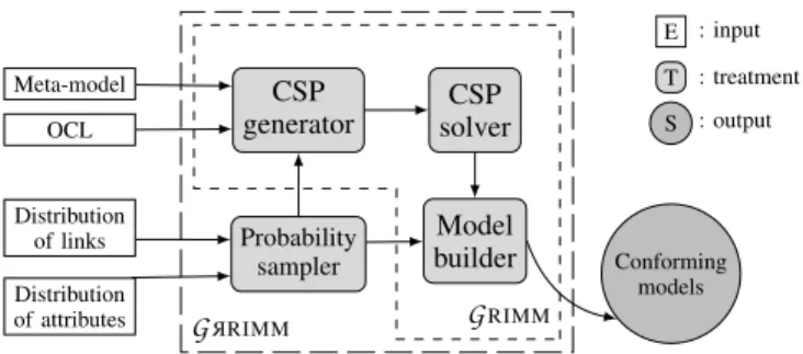
R RIMMtool [9]. Schema on Figure 1 shows the steps for model generation usingG
R RIMMtool. Constraint Programming provides a deterministic behav-ior for the generation, it is then difficult to encode diversity directly in the heart of the tool. Other model generation tools can be coupled with our approach. For example, during our experiment we also used models that have been generated using PRAMANA tool (Sen et al. [2]).
Our contributions are: (1) novel metrics measuring model differences using distances coming from different fields (data mining, code correction algorithms and graph) and adapted to Model Driven Engineering (MDE) (2) solutions to handle a whole set of models in order to compare them, to extract the most representative models inside it and to give a graphical viewing for the concept of diversity in MDE (3) A tool imple-menting these two previous contributions (4) an application of these distance metrics in improving diversity in MDE using a
Meta-model OCL Distribution of links Distribution of attributes Probability sampler CSP generator Model builder CSP solver G R RIMM GRIMM Conforming models E T S : input : treatment : output
Figure 1. Steps for model generation usingGRIMM/G R RIMMtool.
genetic algorithm.
The rest of the paper is structured as follows. Section II details the considered model comparison metrics. Section III details the solutions for handling a set of models (comparison, selection of representative model and graphical viewing). The tool implementing these contributions is described in section IV. An application of our method to the problem of improving diversity in MDE is shown in Section V. Section VI relates about previous work. Section VII concludes the paper.
II. MEASURING MODEL DIFFERENCES
Brun and Pierantonio state in [10] that the complex problem of determining model differences can be separated into three steps: calculation (finding an algorithm to compare two models), representation (result of the computation being represented in manipulable form) and visualization (result of the computation being human-viewable).
Our comparison method aims to provide solutions to com-pare not only two models between them but a whole set of models or sets of models. The rest of this section describes in details the calculation algorithms we choose to measure model differences. Since our method aims to compare sets of models, we took care to find the quickest algorithms. Because chosen comparison algorithms are called hundreds of time to manipulate one set containing dozens of models.
As a proof of concept, we consider here four different distances to express the pairwise dissimilarity between models. As stated in [11], there is intrinsically a difficulty for model metrics to capture the semantics of models. However, formaliz-ing metrics over the graph structure of models is easy, and they propose ten metrics using a multidimensional graph, where the multidimensionality intends to partially take care of semantics on references. They explore the ability of those metrics to characterize different domains using models. In our work, we focus on the ability of distances to seclude models inside a set of models. Thus, we have selected very various distances, essentially of 2 different area: distances on words (from data mining and natural language processing) and distances on graphs (from semantic web and graph theory). Word distances have the very advantage of a quick computation, whereas graph distances are closer to the graph structure of models. As already said, an interesting feature is the fact that all those distances are, in purpose, not domain-specific, not especially coming from MDE, but adapted to the latter.
A. Words distances for models
We define two distances for models based on distances on words: the hamming distance and the cosine distance. The first one is really close to syntax and count the number of difference between two vectors. The second one is normalized and intends to capture the multidimensional divergence between two vectors representing geometrical positions.
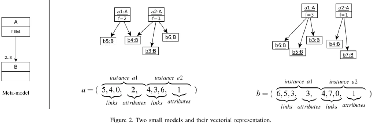
1) From models to words: We define the vectorial represen-tation of a model as the vector collecting links and attributes’ values of each class instance, as illustrated on the model of Fig-ure 2. At the left-hand-side of the figFig-ure is an example of meta-model. At the right-hand-side of the figure are two models conform to this meta-model, and their vectorial representation. The obtained vector from a model m is composed of successive sections of data on each instance of m, when data is available. Each section of data is organized as follows: first data on links, then data on attributes. When there is no such data for a given instance, it is not represented. In the example of Figure 2, instances of B, which have no references and no attributes, as imposed by the meta-model, are not directly represented in the vectors. However, they appear through the links attached to instances of A. An attribute is represented by its value. A link from an instance i to an instance j is represented by the number of the referenced instance j. Each instance of a given meta-class mc, are represented by sections of identical size. Indeed, all the instances of mc have the same number of attributes. The number of links may vary from an instance to another, but a size corresponding to maximal cardinality is systematically attributed. This cardinality is either found in the meta-model or given in the generation parameters. When the actual number of links is smaller than the maximal number of links, 0 values are inserted.
2) Hamming distance for models: Hamming distance com-pares two vectors. It was introduced by Richard Hamming in 1952 [12] and was originally used for fault detection and code correction. Hamming distance counts the number of differing coefficients between two vectors.
The models to compare are transformed into vectors, then we compare the coefficients of vectors to find the distance between both models:
a = (5, 4, 0, 2, 4, 3, 6, 1) b = (6, 5, 3, 3, 4, 7, 0, 1) d(a,b) = 1+ 1+ 1+ 1+ 0+ 1+ 1+ 0
= 68
Richard Hamming’s original distance formula is not able to detect permutations of links, which leads to artificially higher values than expected. In our version, we sort the vectors such as to check if each link exists in the other vector. In the previous example, the final distance then equals to 58. The complexity is linear in the size of models, due to the vectorization step. Notice also that this distance implies that vectors have equal sizes. This is guaranteed by the way we build those vectors.
Meta-model a= ( instance a1 z }| { 5, 4, 0, | {z } links 2, |{z} attributes instance a2 z }| { 4, 3, 6, | {z } links 1 |{z} attributes ) b= ( instance a1 z }| { 6, 5, 3, | {z } links 3, |{z} attributes instance a2 z }| { 4, 7, 0, | {z } links 1 |{z} attributes )
Figure 2. Two small models and their vectorial representation.
3) Cosine distance: Cosine similarity is a geometric mea-sure of similarity between two vectors, ranging from -1 to 1: two similar vectors have a similarity that equals 1 and two diametrically opposite vectors have a cosine similarity of −1. Cosine similarity of two vectors a and b is given by the following formula: CS(a, b) = a.b ||a||.||b||= n ∑ i=1 ai.bi r n ∑ i=1 a2i. rn ∑ i=1 b2i
After a vectorization of models, cosine similarity is then used to compute a normalized cosine distance over two vec-tors [13]:
CD(a, b) =
1 −CS(a, b)
2
Again, the time complexity of the computation is linear in the size of models.
4) Levenshtein distance for models: Levenshtein distance [14] (named after Vladimir Levenshtein) is a string metric used to compare two sequences of characters. To summarise the original idea, a comparison algorithm counts the minimal number of single-character edits needed to jump from a first string to a second one. There exist three character edit operations: addition, deletion and substitution.
Our customized Levenshtein distance is based on the vectorial representation of a model. Each character in original distance is replaced by a class instance of the model. So, we count the minimal cost of class instance edit operations (addition, deletion or substitution) to jump from the first model to the second one.
First, a vectorial representation of a model is created according to the class diagram given in Figure 3. Then, we determine the cost of each one of the three edit operations over instanceOfClass objects. instanceCost method gives the cost to add or to delete an instanceOfClass. It counts the number of edges and the number of attributes of this instance. substituCost method gives the cost to substitute an instance by another one. To determine the substitution cost, we count the number of common links and attributes. Thus, two instanceOfClass are exactly equal if they have the same
Figure 3. Class diagram for instanceOfClass and Link to build a vectorial representation of a model.
type, their links have the same type and all their attributes have the same values.
Finally, Levenshtein algorithm [14] is applied and a metric of comparison is computed. Our comparison metric gives the percentage of common elements between two models.
B. Centrality distance for models
Centrality is a real function that associates a value to each node of a graph [15]. This value indicates how much a node is central in this graph, according to a chosen criterion. For example, in a tree, the highest value of centrality is given to the root of the tree, whereas the smallest values are associated to the leaves. A centrality function C is defined by:
C: E→ R+ v7→ C(v)
Many usual centrality functions exist. The simplest one, the degree centrality, associates to each node its degree. Among the well-known centrality functions, we can cite: betweenness centrality, closeness centrality, harmonic centrality, etc.
In this paper, we propose a novel centrality function adapted for MDE and based on eigenvector centrality. This centrality was also used in the first published version of PageRank algorithm of the Google search engine [16]. In PageRank, eigenvector centrality is used to rank the web pages taken as nodes of the same graph.
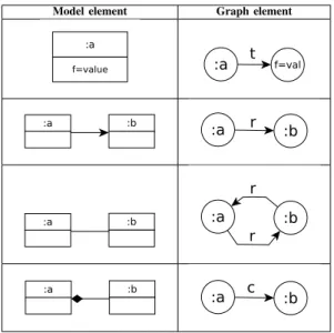
1) From models to graphs: Centrality functions are defined on graphs, and models could be considered as labelled and typed graphs. Our graph representation of models is obtained as follows:
TABLE I. NODES TRANSFORMATION RULES.
Model element Graph element
TABLE II. EDGES TRANSFORMATION RULES.
Model element Graph element
• Create a node for each class instance (central nodes). • Create a node for each attribute (leaf nodes). • Create an edge from each class instance to its
at-tributes.
• Create an edge for each simple reference between two class instances.
• Create two edges if two class instances are related by two opposite references.
• Create an edge for each composition link.
Tables I and II summarize and illustrate these transforma-tions rules. Real numbers c, r and t represent the weights assigned to composition links, reference links and attributes.
2) Centrality measure: Our centrality is inspired from pagerank centrality and adapted to models, taking into ac-count class instances and their attributes, links between classes (input and output) and types of link between two classes (simple references, two opposite references or compositions). For a given node v of the graph, we denote by N(v) the set of its neighbors. The following function gives the centrality of each node v:
C(v) =
∑
u∈N+(v)
C(u)
deg(u)× w(v, u).
w(v, u) gives the weight of the link between node v and u, determined by the kind of link between them (attribute, reference or composition). The weight of a link can be given by the user or deduced from domain-based quality metrics. For instance, Kollmann and Gogolla [17] described a method for creating weighted graphs for UML diagrams using object-oriented metrics.
3) Centrality vector: The centrality vector C contains the values of centrality for each node. The previous centrality func-tion induces the creafunc-tion of a system of n variables equafunc-tions: C(vi) = c1C(v1) + c2C(v2) + . . . + ciC(vi) + . . . + cnC(vn).
To compute the centrality vector C we must find the eigenvector of a matrix A whose values are the coefficients of the previous equations: C= AC, where A is built as follows:
Ai j= 0 if(vi, vj) /∈ Graph, w(vi, vj) N(vi) otherwise.
After building matrix A, we use the classical algorithm of power iteration (also known as Richard Von Mises method [18]) to compute the centrality vector C.
The result centrality vector has a high dimension (see example on Figure 4). To reduce this dimension therefore improve the computation’s efficiency, we group its coefficients according to the classes of the meta-model. Then the dimen-sion equals to the number of classes in the meta-model.
4) Centrality distance: Roy et al. proved in [19] that a centrality measure can be used to create a graph distance. Here, the centrality vectors CA and CB of two models A and B are
compared using any mathematical norm: d(A, B) = ||CA−CB||.
C. Discussion
We use in previous paragraphs representations of models which could be discussed. Indeed, there are potentially many ways to vectorize models, and we choose one highly com-patible with our tool. Since CSP generation already provides a list of classes attributes and links, we simply used this representation as entry for the metrics. Again, transforming models into graphs and trees may be done through several ways. We arbitrarily choose one way that seemed to capture the graph structure. Our goal here, was to test different and diversified manners to represent a model and proposed some distance between them, not to make an exhaustive comparison study between quality of representation versus metrics. This study will be done in future works.
III. HANDLING SETS OF MODELS
In this section, we propose an automated process for handling model sets. The purpose is to provide solutions for comparing models belonging to a set, selecting the most representative models in a set and bringing a graphical view of the concept of diversity in a model set.
This process helps a user in choosing a reasonable amount of models to perform his experiments (e.g., testing a model transformation). Moreover, using our approach, the chosen
Meta-model
Figure 4. Centrality vector computed for an example model and its equivalent graph.
model set aims to achieve a good coverage of the meta-model’s solutions space.
If there are no available models, a first set of models is generated using
G
R RIMM tool [9]. These generated models are conform to an input meta-model and respect its OCL constraints. When probability distributions related to domain-specific metrics are added to the process, intra-model diversity is improved. Our goal is to check the coverage of the meta-model’s solutions space. In other words, we want to help a user to answer these questions: (1) how to quantify the inter-model diversity ? (2) Are all these models useful and representative ? (3) Which one of my model sets is the most diverse ? A. Comparison of model setsDistance metrics proposed in Section II compare two models. To compare a set of models, we have to compute pair-wise distances between models inside the set. A symmetrical distance matrix is then created and used to quantify the inter-model diversity. It is noticeable that, thanks to the modularity of the approach, this step can be replaced by any kind of dataset production. For instance, if the user already has a set of models, it is possible to use it instead of the generated one. Moreover, another distance metric can be used instead of the metrics we propose.
B. Selecting most representative models
Our idea is that when a user owns a certain number of models (real ones or generated ones), there are some of them which are representative. Only these models should be used in some kind of tests (e.g., robustness or performance). Most of other models are close to these representative models.
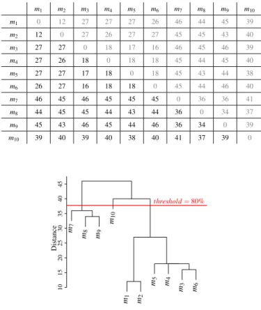
We use Hierarchical Matrix clustering techniques to select the most representative models among a set of models. The distance matrix is clustered and our tool chooses a certain num-ber of models. In our tool, we use the hierarchical clustering algorithm [20], implemented in the R software (hclust, stats package, version 3.4.0) [21]. This algorithm starts by finding a tree of clusters for the selected distance matrix as shown in Figure 5. Then, the user has to give a threshold value in order to find the appropriate value. This value depends on the diversity the user wants. For example, if the user wants models sharing only 10% of common elements, then 90% is the appropriate threshold value. This value depends also on the used metric. Thus, Levenshtein distance compares the names of elements and the values of attributes, leading to choose a smaller threshold value (for the same model set) than for
centrality distance which compares only the graph structure of the models.
Using the clusters tree and the threshold value, it is easy to derive the clusters, by cutting the tree at the appropriate height (Figure 5). The most representative models are chosen by arbitrarily picking up one model per cluster. For instance, 3 different clusters are found using the tree of clusters in Figure 5. Clone detection can also be performed using our approach by choosing the appropriate threshold value. Indeed, if threshold equals to 0, clusters will contain only clones.
TABLE III. AN EXAMPLE OF DISTANCE MATRIX (HAMMING) FOR 10 MODELS. m1 m2 m3 m4 m5 m6 m7 m8 m9 m10 m1 0 12 27 27 27 26 46 44 45 39 m2 12 0 27 26 27 27 45 45 43 40 m3 27 27 0 18 17 16 46 45 46 39 m4 27 26 18 0 18 18 45 44 45 40 m5 27 27 17 18 0 18 45 43 44 38 m6 26 27 16 18 18 0 45 44 46 40 m7 46 45 46 45 45 45 0 36 36 41 m8 44 45 45 44 43 44 36 0 34 37 m9 45 43 46 45 44 46 36 34 0 39 m10 39 40 39 40 38 40 41 37 39 0 m7 m8 m9 m10 m1 m2 m5 m4 m3 m6 10 15 20 25 30 35 40 45 Distance threshold= 80%
Figure 5. Clustering tree computed form matrix in Table III.
C. Graphical view of diversity
Estimating diversity of model sets is interesting for model users. It may give an estimation on the number of models
needed for their tests or experiments and they can use this diversity measure to compare between two sets of models.
When the number of models in a set is small, diversity can be done manually by checking the distance matrix. Unfortu-nately, it becomes infeasible when the set contains more than an handful of models. We propose a human-readable graphical representation of diversity and solutions’ space coverage for a set of models. m1m2 m3 m4 m5 m6 m7 m8 m9 m10
Figure 6. Voronoi diagram for 10 models compared using Hamming distance.
Our tool creates Voronoi tessellations [22] of the distance matrix in order to assist users in estimating the diversity or in comparing two model sets. A Voronoi diagram is a 2D representation of elements according to a comparison criterion, here distances metrics between models. It faithfully reproduces the coverage of meta-model’s solutions space by the set of models. Figure 6 shows the Voronoi diagram created for the matrix in Table III. The three clusters found in the previous step are highlighted by red lines. We use the Voronoi functions of R software (available in package tripack, v1.3-8).
IV. TOOLING
This section details the tooling implementing our con-tributions. All the algorithms and tools are in free access and available on our web pages: http://adel-ferdjoukh.ovh/index.php/research/.
Our tool for comparing models and handling model sets is called COunting MOdel DIfferences (COMODI). It consists in two different parts. The first one, written in java, is used to measure differences between two models using the above 4 metrics. The second part, written in bash and R, provides algorithms for handling model sets (comparison, diversity estimation and clustering).
A. Comparing two models
It is possible to measure the differences between two models using COMODI. For that you just need to give as input two models and their ecore meta-model. Out tool supports two different formats: dot model files produced by
G
RIMMand xmi model files. COMODIsupports all xmi files produced by EMF of generated byG
RIMM, EMF2CSP or PRAMANAtools.The first step is to parse the input models into the ap-propriate representation (graph or vector). Then, the above distance algorithms are applied. COMODI outputs different model comparison metrics in command line mode. Process of COMODI is described in figure 7.
Meta-model Model 1 Model 2
Xmi or dot parsers
Levenshtein distance Hamming distance
Cosine distance Centrality distance
Figure 7. Comparing two models usingCOMODItool.
B. Handling a set of models
Our tool is also able to handle sets of models and produce distance matrices, perform clustering and plot diagrams and give some statistics. The input of the tool is a folder containing the models to compare and their ecore meta-model. The supported formats for models are the same as described above (xmi and dot).
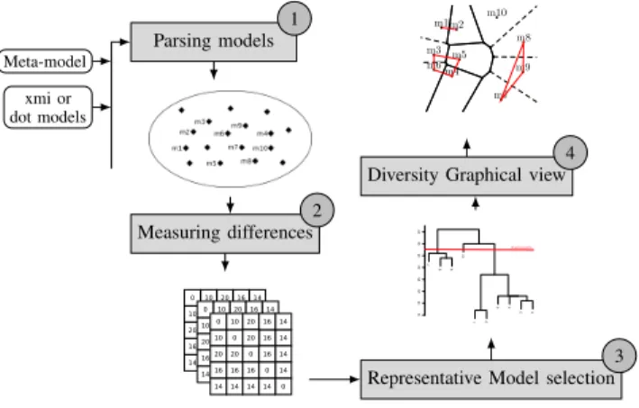
Meta-model xmi or dot models Parsing models 1 Measuring differences 2
Representative Model selection 3 7 8 9 10 1 2 5 4 3 6 10 15 20 25 30 35 40 45 threshold=80%
Diversity Graphical view 4 m1m2 m3 m4 m5 m6 m7 m8 m9 m10
Figure 8. Handling a set of models usingCOMODItool.
After parsing all the models into the appropriate repre-sentation for each metric, distance matrices are produced by pairwise comparison of models. R scripts are called to perform hierarchical clustering on these matrices. This allows us to select the most representative models of that folder. Voronoi diagrams are plotted and can be used to estimate the coverage of the folder and to compare the diversity of two folders.
COMODI prints also some simple statistics on models: closest models, most different models, etc. These steps are shown in figure 8.
V. APPLICATION: IMPROVING DIVERSITY
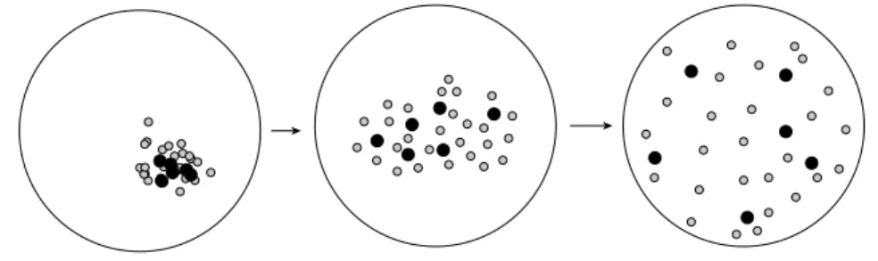
The main contributions of this paper - distances between models, representative model selection to improve diversity -were used in a work in bioinformatics (named scaffolding). A genetic approach is paired with
G
R RIMMmodel generation tool to improve the diversity of a set of automatically generated models. Figure 9 shows how we start from aG
RIMMmodel set (left) with few difference between them, toG
R RIMM (center) with a better distribution due to the probability sampler, to something very relevant by using a genetic approach (right) based on these model distances in order to improve diversity. We want to address the following question: do proposed distances and process of automated models selection help toFigure 9. Diversity improving process. Black circles are the most representative models of the set.
Figure 10. The meta-model of Scaffold graphs.
improve the diversity and the coverage of generated models. We chose one meta-model (Figure 10) modeling a type of graphs involved in the production of whole genomes from new-generation sequencing data [23]. Hereinafter we give the experimental protocol:
• Generate 100 initial models conforming to the scaffold graph meta-model using
G
R RIMM tool [9].• Model the problem of improving diversity using ge-netic algorithms (GA). Our modeling in GA can be found in [24].
• Run 500 times the genetic algorithm. At each step, use model distances and automatic model selection to choose only the best models for the next step. • View final results in terms of model distances and
meta-model coverage using Voronoi diagrams. The whole process induces the creation of up to 50, 000 different models. Each following figures required about 3h CP to be computed.
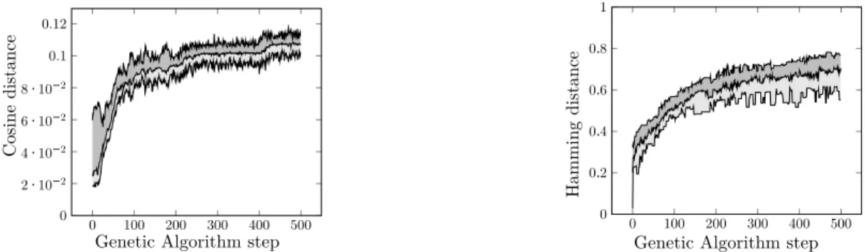
Curves on Figure 11 show the evolution of hamming and cosine distance while the genetic algorithm is running (minimum, maximum and mean distance over the population at each generation). We can observe that both cosine distance and hamming distance help to improve diversity of generated models. The quick convergence of both curves (around 100 iterations of GA) is a good way to check the efficiency of both models distances. We observe that the worst case in the final population is better than the best case in the initial population, thus we reached a diversity level that we did not obtained in the initial population obtained with
G
R RIMM.We introduce several improvements to describe the fitness function used in genetic selection [24] and improve median value for final population from 0.7 up to 0.9 for Hamming and from 0.11 to 0.15 for maximum with Cosinus distance. Figure 12 compares the models produced by the different distances.
Red (resp. blue) dotplots represent the distribution of distances on the final population computed using Hamming distance (resp. Cosine distance). On the left, models are compared using Hamming distance, on the right, they are compared using Cosine distance. We remark that different distances do not produce the same final models. Indeed, we can observe that the best selected models for Hamming distance obtain lower scores when compared using Cosine distance, and vice versa. Other experimental results show that our four model distances can be used in a multi-objective genetic algorithm since they treat different constructions of the meta-model. Results are better on the final model set in terms of diversity and coverage, than when only one kind of distance is used.
Figure 13 shows two Voronoi diagrams of 100 models. The first one is computed on the initial set of models, the second on the set of models generated after the 500th iteration of the genetic algorithm. We kept the same scale to visualize the introduced seclusion. Here we can see the insufficient solutions’ space coverage of the first Voronoi diagram. After running the multi-objective genetic algorithm, we observe a better coverage of the space. At the end of the process, we obtain 100 very distinct models.
VI. RELATED WORK
A. Model comparison
The challenging problem of model comparison was widely studied, many techniques and algorithms were proposed for it. Two literature studies are proposed in [5] and [25]. Among all the techniques, we describe here the techniques that are close to the model distance algorithms we propose, in both comparison and objective.
Falleri et al. [26] propose a meta-model matching approach based on similarity flooding algorithm [27]. The goal of this approach is to detect mappings between very close meta-models to turn compatible meta-models which are conform to these meta-models. The comparison algorithm detects two close meta-models. A transformation is then generated to make the models of the first meta-model conform to the second one. However, in such kind of work, the similarity between models cannot be detected without using the names of elements: lexical similarities are propagated through the structure to detect matchings. Our approach is more structural.
Voigt and Heinze present in [28] a meta-model matching approach. The objective is very close to the previous approach. However, the authors propose a comparison algorithm that is based on graph edit distance. They claim that it is a way
0 100 200 300 400 500 0 2 · 10−2 4 · 10−2 6 · 10−2 8 · 10−2 0.1 0.12
Genetic Algorithm step
Cosine distan ce 0 100 200 300 400 500 0 0.2 0.4 0.6 0.8 1
Genetic Algorithm step
Hamming
distance
Figure 11. Minimum, average and maximum hamming and cosine distance while running the genetic algorithm.
Figure 12. Comparison of best selected models pairwise distances distributions.
Figure 13. Solutions’ space coverage of the initial set of models (left) compared to the last iteration (500th) of the genetic algorithm (right).
to compare the structure of the models and not only their semantics as most of techniques do.
B. Model selection
Cadavid et al. [29] present a technique for searching the boundaries of the modeling space, using a meta-heuristic method, simulated annealing. They try to maximize cov-erage of the domain structure by generated models, while maintaining diversity (dissimilarity of models). In this work, the dissimilarity is based on the over-coverage of modeling space, counting the number of fragments of models which are covered more than once by the generated models in the set. In our work, the objective is not to search the boundaries of the search space but to select representative and diverse elements in the whole search space. More recently, Batot et al. [30] proposed a generic framework based on a
multi-objective genetic algorithm (NSGA-II) to select models sets. The objectives are given in terms of coverage and minimality of the set. The framework can be specialized adding coverage criterion, or modifying the minimality criterion. This work of Batot et al confirms the efficiency of genetic algorithms for model generation purposes. Our work is in the same vein but focuses on diversity.
Hao Wu [31] proposes an approach based on SMT (Sat-isfiability Modulo Theory) to generate diverse sets of models. It relies on two techniques for coverage oriented meta-model instance generation. The first one realizes the coverage criteria defined for UML class diagrams, while the second generates instances satisfying graph-based criteria.
Previous approaches guarantee the diversity relying only on the generation process. No post-process checking is performed on generated model sets to eliminate possible redundancies or to provide a human-readable graphical view of the set.
VII. CONCLUSION
Counting model differences is a recurrent problem in Model Driven Engineering, mainly when sets of models have to be compared. This paper tackles the issue of comparing two models using several kinds of distance metrics inspired from distances on words and distances on graphs. An approach and a tool are proposed to handle sets of models. Distance metrics are applied to those sets. Pair of models are compared and a matrix is produced. We use hierarchical clustering algorithms to gather the closest models and put them in subsets. Our tool,
COMODI, is also able to choose the most representative models of a set and give some statistics on a set of models. Human readable graphical views are also generated to help users in doing that selection manually.
The first application of our contributions is improving diversity when generating models. Sets of non-diverse models are automatically generated. COMODI is coupled to a genetic algorithm to improve the diversity of this first set of models. A. application and future work
The problematic of handling sets of models and the notion of distance is also involved in many other works related to testing model transformations. All these issues are interesting applications to the contributions of this paper. For example, Mottu et al. in [32] describe a method for discovering model transformations pre-conditions by generating test models. A first set of test models is automatically generated and used to execute a model transformation. Excerpts of models that make the model transformation failing are extracted. An expert then tries manually and iteratively to discover pre-conditions using these excerpts. Our common work aims to help the expert by reducing the number of models excerpts and the number of iterations to discover most of pre-conditions. A set of models excerpts is handled usingCOMODIand clusters of close models are generated. Using our method, the expert can find many pre-conditions in one iteration and using less model excerpts.
Future work will consist in performing large experiments involving and comparing other kinds of distances, and to measure to what extend the way models are encoded into other structures (e.g., words or trees) affects the results. We remark that metrics and distances have also very different effects on the evolution of the models set, and intend to further investigate and characterize this phenomenon.
REFERENCES
[1] A. Ferdjoukh, A.-E. Baert, A. Chateau, R. Coletta, and C. Nebut, “A CSP Approach for Metamodel Instantiation,” in IEEE ICTAI, 2013, pp. 1044–1051.
[2] S. Sen, B. Baudry, and J.-M. Mottu, “Automatic Model Generation Strategies for Model Transformation Testing,” in ICMT, International Conference on Model Transformation, 2009, pp. 148–164.
[3] C. A. Gonz´alez P´erez, F. Buettner, R. Claris´o, and J. Cabot, “EMFtoCSP: A Tool for the Lightweight Verification of EMF Models,” in FormSERA, Formal Methods in Software Engineering, 2012, pp. 44–50.
[4] F. Hilken, M. Gogolla, L. Burgue˜no, and A. Vallecillo, “Testing models and model transformations using classifying terms,” Software & Systems Modeling, 2016, pp. 1–28.
[5] D. S. Kolovos, D. Di Ruscio, A. Pierantonio, and R. F. Paige, “Different models for model matching: An analysis of approaches to support model differencing,” in CVSM@ICSE, 2009, pp. 1–6.
[6] D. Steinberg, F. Budinsky, M. Paternostro, and E. Merks, EMF: Eclipse Modeling Framework 2.0. Addison-Wesley Professional, 2009. [7] A. Ferdjoukh, A.-E. Baert, E. Bourreau, A. Chateau, and C. Nebut,
“In-stantiation of Meta-models Constrained with OCL: a CSP Approach,” in MODELSWARD, 2015, pp. 213–222.
[8] F. Rossi, P. Van Beek, and T. Walsh, Eds., Handbook of Constraint Programming. Elsevier Science Publishers, 2006.
[9] A. Ferdjoukh, E. Bourreau, A. Chateau, and C. Nebut, “A Model-Driven Approach to Generate Relevant and Realistic Datasets,” in SEKE, 2016, pp. 105–109.
[10] C. Brun and A. Pierantonio, “Model differences in the eclipse modeling framework,” UPGRADE, The European Journal for the Informatics Professional, vol. 9, no. 2, 2008, pp. 29–34.
[11] G. Sz´arnyas, Z. Kov´ari, ´A. Sal´anki, and D. Varr´o, “Towards the char-acterization of realistic models: evaluation of multidisciplinary graph metrics,” in MODELS, 2016, pp. 87–94.
[12] R. W. Hamming, “Error detecting and error correcting codes,” Bell System technical journal, vol. 29, no. 2, 1950, pp. 147–160. [13] A. Singhal, “Modern information retrieval: A brief overview,” IEEE
Data Engineering Bulletin, vol. 24, no. 4, 2001, pp. 35–43.
[14] V. Levenshtein, “Binary codes capable of correcting deletions, inser-tions, and reversals,” in Soviet physics doklady, vol. 10, no. 8, 1966, pp. 707–710.
[15] G. Kishi, “On centrality functions of a graph,” in Graph Theory and Algorithms. Springer, 1981, pp. 45–52.
[16] L. Page, S. Brin, R. Motwani, and T. Winograd, “The PageRank citation ranking: bringing order to the web,” Stanford InfoLab, Tech. Rep., 1999. [17] R. Kollmann and M. Gogolla, “Metric-based selective representation of
uml diagrams,” in CSMR. IEEE, 2002, pp. 89–98.
[18] R. von Mises and H. Pollaczek-Geiringer, “Praktische verfahren der gleichungsaufl¨osung.” ZAMM-Journal of Applied Mathematics and Mechanics, vol. 9, no. 2, 1929, pp. 152–164.
[19] M. Roy, S. Schmid, and G. Tr´edan, “Modeling and measuring Graph Similarity: the Case for Centrality Distance,” in FOMC, 2014, pp. 47– 52.
[20] F. Murtagh, “Multidimensional clustering algorithms,” Compstat Lec-tures, Vienna: Physika Verlag, 1985, 1985.
[21] R Development Core Team, R: A Language and Environment for Statistical Computing, R Foundation for Statistical Computing, 2008. [22] F. Aurenhammer, “Voronoi diagrams a survey of a fundamental
geometric data structure,” CSUR, ACM Computing Surveys, vol. 23, no. 3, 1991, pp. 345–405.
[23] M. Weller, A. Chateau, and R. Giroudeau, “Exact approaches for scaffolding,” BMC Bioinformatics, vol. 16, no. 14, 2015, pp. 1471– 2105.
[24] F. Galinier, E. Bourreau, A. Chateau, A. Ferdjoukh, and C. Nebut, “Genetic Algorithm to Improve Diversity in MDE,” in META, 2016, pp. 170–173.
[25] Voigt, Konrad, “Structural Graph-based Metamodel Matching,” Ph.D. dissertation, Dresden University, 2011.
[26] J.-R. Falleri, M. Huchard, M. Lafourcade, and C. Nebut, “Metamodel matching for automatic model transformation generation,” in MODELS, 2008, pp. 326–340.
[27] S. Melnik, H. Garcia-Molina, and E. Rahm, “Similarity flooding: A versatile graph matching algorithm and its application to schema matching,” in ICDE, 2002, pp. 117–128.
[28] K. Voigt and T. Heinze, “Metamodel matching based on planar graph edit distance,” in Theory and Practice of Model Transformations, 2010, pp. 245–259.
[29] J. Cadavid, B. Baudry, and H. Sahraoui, “Searching the Boundaries of a Modeling Space to Test Metamodels,” in IEEE ICST, 2012, pp. 131–140.
[30] E. Batot and H. Sahraoui, “A Generic Framework for Model-set Selection for the Unification of Testing and Learning MDE Tasks,” in MODELS, 2016, pp. 374–384.
[31] H. Wu, “An SMT-based Approach for Generating Coverage Oriented Metamodel Instances,” IJISMD, International Journal of Information System Modeling and Design, vol. 7, no. 3, 2016, pp. 23–50. [32] J.-M. Mottu, S. Sen, J. Cadavid, and B. Baudry, “Discovering model
transformation pre-conditions using automatically generated test mod-els,” in ISSRE, 2015, pp. 88–99.