A surface registration method for quantification of intraoperative brain deformations in image-guided neurosurgery.

HAL Id: inserm-00546498

https://www.hal.inserm.fr/inserm-00546498

Submitted on 14 Dec 2010

HAL is a multi-disciplinary open access

archive for the deposit and dissemination of

sci-entific research documents, whether they are

pub-lished or not. The documents may come from

teaching and research institutions in France or

abroad, or from public or private research centers.

L’archive ouverte pluridisciplinaire HAL, est

destinée au dépôt et à la diffusion de documents

scientifiques de niveau recherche, publiés ou non,

émanant des établissements d’enseignement et de

recherche français ou étrangers, des laboratoires

publics ou privés.

intraoperative brain deformations in image-guided

neurosurgery.

Perrine Paul, Xavier Morandi, Pierre Jannin

To cite this version:

Perrine Paul, Xavier Morandi, Pierre Jannin. A surface registration method for quantification of

intraoperative brain deformations in image-guided neurosurgery.. IEEE Transactions on Information

Technology in Biomedicine, Institute of Electrical and Electronics Engineers, 2009, 13 (6), pp.976-83.

�10.1109/TITB.2009.2025373�. �inserm-00546498�

Abstract— Intraoperative brain deformations decrease accuracy in image-guided neurosurgery. Approaches to quantify these deformations based on 3D reconstruction of cortectomy surfaces have been described and have shown promising results regarding the extrapolation to the whole brain volume using additional prior knowledge or sparse volume modalities. Quantification of brain deformations from surface measurement requires the registration of surfaces at different times along the surgical procedure, with different challenges according to the patient and surgical step. In this paper, we propose a new flexible surface registration approach for any textured point cloud computed by stereoscopic or laser range approach. This method includes three terms: the first term is related to image intensities, the second to Euclidean distance and the third to anatomical landmarks automatically extracted and continuously tracked in the 2D video flow. Performance evaluation was performed on both phantom and clinical case. The global method, including textured point cloud reconstruction, had accuracy within 2 millimeters, which is the usual rigid registration error of neuronavigation systems before deformations. Its main advantage is to consider all the available data, including the microscope video flow with higher temporal resolution than previously published methods.

Index Terms—Image-Guided Neurosurgery, Intraoperative Brain Surface Deformation, Video Analysis, Surface Registration

I. INTRODUCTION

NTRAOPERATIVE _{brain deformations decrease accuracy in image guided neurosurgery. Image guided neurosurgery (IGNS) is}

based on the registration between pre operative images and the patient coordinate space using external landmarks or skin surface [1]. This registration relies on a rigid transform assumption, which is not verified during some neurosurgical procedures for the brain. For surgical tumor resection, many parameters may influence brain deformations, e.g. gravity, lesion size, loss of cerebro-spinal fluid, resection [2]. As shown in [3], amplitude of these deformations can be up to 3 centimeters, they are not uniform, and their principal direction is not always the gravity direction. Lot of effort has been deployed for updating preoperative images according to the intraoperative deformations. Developed approaches are usually based on intraoperative imaging, e.g. three-dimensional ultrasound [4]-[8], surface acquisition [9]-[14], interventional MRI [15]-[17], with possible use of biomechanical models [13]-[15], [18]-[21] or predictive models [5], [22]. However, there are some remaining issues concerning computation time, costs of technology and user interface. Surface information is one interesting solution to cope with these issues, especially for updating regions of interest near the cortical surface, as tumor, functional areas, vessels and sulci [23]. It has also been shown that volumetric brain deformation can be inferred given the cortical surface displacement [9], [10], [13], [14], and [24].

Cortical surface can be acquired using stereoscopic [12], [13], [25], or laser range scanning approaches [9], [11]. The data set then consists in textured point clouds. For accurate quantification of the cortical surface displacement, a robust non-rigid surface registration method of these dataset is required. In [26], different surface registration methods for the same type of data were compared: feature based registration, cortical vessel-contour registration, a combined geometry-intensity surface registration method, based on the use of mutual information (MI), and a form of the former method which was constrained by manually identified sparse landmarks in order to improve robustness. The conclusion of the study was that the methods performed differently according to the patient and the particular clinical case, but that the constrained form of the geometry-intensity surface registration method was generally outperforming all other studied methods.

Surgical tools or bleeding may suddenly appear in the images from the operative FOV, which may hamper MI based image registration. Moreover, surfaces acquired before the dura mater opening do not offer the same texture information than surface acquired after dura mater opening. In that case, only the geometric information can be used.

Manuscript received March 18, 2009.

A Surface Registration Method for

Quantification of Intraoperative Brain

Deformations in Image-Guided

Neurosurgery

Perrine Paul, Xavier Morandi, and Pierre Jannin, Member, IEEE

In a previous publication, we introduced and evaluated a method for computing 3D surfaces of the operative field viewed through the oculars of a surgical microscope by using stereoscopic reconstruction methods [25]. In this paper, we propose a new non-rigid registration method for registering such 3D surfaces, which allows a flexible computation of a dense transformation field thanks to a weighted combination of geometric information, texture matching, and sparse landmarks matching. One of the novelties of our method is that the landmarks are automatically extracted and tracked in the video flow between two surface acquisitions. Up to our knowledge, the previously published methods neither used the video flow as a source of information nor an automatic extraction and matching of landmarks.

In the next sections, we describe this new surface registration method for matching two reconstructed surfaces and demonstrate its implementation in clinical settings. We first describe the automatic extraction of the anatomical landmarks as well as the method for video tracking. We then introduce the new cost function. Performance evaluation of video tracking and of the registration method is described on both phantom and patient, showing the clinical feasibility of our approach.

II. MATERIALS AND METHODS

The image acquisition and surface registration workflow was repeated for each one of the deformation estimation (Fig. 1). At surgical time ti, a pair of video static images, as seen through the surgical microscope binoculars, was acquired as explained in subsection II-A. Stereoscopic reconstruction methods were applied on these images and provided a 3D surface of the operative field as explained in [25]. At time ti, anatomical landmarks were automatically extracted from the right image as explained in subsection II-B. Video flow from the right ocular was continuously acquired from times ti to tj. The extracted anatomical landmarks were continuously tracked in the 2D images from the video flow using the method described in subsection II-C. At time tj, a new pair of video images was acquired and a new surface was reconstructed. Matching of both ti and tj surfaces was performed using the proposed surface registration method, described in section II-D.

A. Acquisition

A stereovision system (Zeiss 3-D Compact Video Camera S2, Carl Zeiss, Germany) was set up between the NC4 surgical microscope and the binocular tube. Images from these analog cameras were acquired using a video acquisition card (PICOLO, Euresys, Belgium). The operative room was also equipped with a neuronavigation system (StealthStation, Medtronic SNT, USA).

Each acquisition consisted of:

- At time ti, one static pair of images from both left and right surgical microscope oculars, along with position and settings of the microscope,

- A 2D video flow from the right ocular, whose first frame was the static right image at ti , and whose last frame was the static right image at time tj,

- At time tj, one static pair of images from both left and right surgical microscope oculars, along with position and settings of the microscope.

Fig. 1. Image acquisition and surface registration workflow.

Positions and settings of the microscope were obtained using the neuronavigation system and a communication library (StealthLink, Medtronic SNT, USA). Cortical surfaces were computed by dense reconstruction of microscope stereoscopic images as explained in [25]. We obtained two surface meshes, one at time ti andone at time tj. Each surface mesh was textured by the right image from the surgical microscope [25]. All images from microscope oculars have a resolution of 768X576 pixels.

B. Extraction of landmarks in right image

First, a mathematical morphological opening with a square element of size 10x10 and a Laplacian of Gaussian filter was applied on the right image I acquired at time ti in order to detect the boundaries of the operative field (see Fig. 2). The operative field was roughly segmented from the filtered image Ip by the following method for limiting the anatomical landmarks detection to the cortical surface area. It was scanned horizontally from left to right then from right to left in order to locate 255-luminance-level pixels first met in each direction. These pixels defined the bends of the first mask. A new square mask of size 400 pixels was then defined. The center of this mask was defined as the gravity center of the first mask after a mathematical morphology opening. The convolution of this new mask and Ip was scanned as previously explained to segment the operative field. A mathematical morphology opening was then applied to the scanned image to obtain the final mask.

Fig. 2. Pre processing steps and natural landmark extraction. Top left: original image, top right after morphological opening; bottom left: after laplacian of Gaussian; bottom right: the mask is computed from the laplacian of Gaussian, and applied to the original image, from which are extracted the natural landmarks.

Fig. 3. Results in clinical settings on patient: anatomical landmarks extracted automatically: the 15 best landmarks only (15 maxima values of Harris extractor) after having removed specularities.

The detection of the landmarks was based on the Harris detector [27], applied on the segmented image Ic , taking the local maxima of the following expression R:

(1) with λ=0.04 as often chosen in the literature, and

,

where det(M) and Tr(M) stand for the determinant and the trace of the matrix M, respectively, and x and y are coordinates of pixels in Ic. Among these local maxima, points with intensity higher than 80% of the maximal intensity of the image were rejected to eliminate specularities. The result of this final step was a file with the 2D coordinates of landmarks in the static right image.

An example of result from this step is shown in Fig. 3.

C. Tracking of landmarks from video flow

The position of the landmarks in each image of the video flow between ti and tj was considered as a dynamic system, modeled as a hidden Markov process. The goal was to estimate the values of the state xk from observations zk obtained at each instant, k defined as an integer in ]i,j]. The system was described by a dynamic equation modeling the evolution of the state and a measurement model that links the observation to the state. We considered the unknown state of the system as the landmark position in the present and in the previous instant.

1) Measurement model: At time k, we assumed that the observation was the result of a matching process whose goal is to

provide the point in image Ik that is the most similar to the initial point x0. We used sum-of-squared-differences (SSD) as matching criteria for quantifying the similarity between the target point and the candidate points. The resulting linear observation equation is:

. (2)

The state xk was defined by (mk−1,mk,nk−1,nk)T , where (mk,nk)T is the feature location at time k, zk is the measure obtained by SSD at times k and k-1, and wk is a zero-mean Gaussian white noise of covariance Rk. This equation models the noise associated to the measure by a Gaussian wk. Despite possible difficulties with illumination or geometric changes, this choice of SSD was justified in [28] by possible automatic evaluation of the confidence in the correlation peak (i.e., of Rk), taking into account the image noise. For that purpose, the SSD surface centered on zk was modeled as a probability distribution of the true match location [28]. A Chi-Square “‘goodness of fit” test was used to check when this distribution was locally better approximated by a Gaussian or a uniform law [28]. An approximation by a Gaussian distribution indicated a clear discrimination of the measure and

Rk was set to the local covariance of the distribution. On the contrary, an approximation by a uniform distribution indicated unclear peak detection on the response distribution. This can be explained by occlusions or noisy situations. In such cases, the diagonal terms of Rk were fixed to infinity, and the off-diagonal terms were set to 0. This estimation allowed the tracker to be robust to occlusions.

2) Dynamic model: The following dynamic equations have been considered:

, (3)

where vk is a zero-mean Gaussian white noise of covariance fixed a priori and l the index of the process (F, b). We defined two process models corresponding to different surgical steps.

, ,

and , , (4)

where (mi, ni)T is the feature location at time ti. The model (F1, b1) relies on a stationary hypothesis. It was used when brain movements were expected to be very regular and when there was no surgical tool used in this surgical step. The model (F2, b2) is a regressive process of 2nd order. It was used to take into account quick non-linear movements, especially when surgical tools were used and deformed the brain surface.

The resulting systems were linear and were solved using the Kalman filter [29]. This tracker was used to follow the extracted landmarks in the video. The tracking stage resulted in a file containing landmarks positions in the right picture used to compute stereoscopic reconstruction at ti and at tj. A confidence value expressed as the variance of the posterior probability density used to compute the state estimate for each landmark tracker was associated to each landmark-tracked position.

D. Surface registration

The cortical surface deformation was quantified by a dense deformation field computed by registration between two surface meshes.

1) Initialization: Thanks to the stereoscopic reconstruction and calibration, the coordinates of the tracked landmarks at times ti and tj were automatically defined in a common coordinate system [25] as 3D points, and respectively, n being the index of the extracted and tracked landmark. This automatic correspondence was used to compute a sparse surface deformation field. From this sparse deformation field, an initial dense deformation field Dfinit was computed by Thin-Plate-Spline interpolation using anatomical landmarks as control points [30].

2) Cost function: The cost function F included three terms and two weighting factors α and β (4). The first term A was related

to image intensities, the second B to Euclidean distance between surfaces and the third C to distance between tracked landmarks. Equation (5) defines F for any 3D point Pi from the surface mesh at time ti and a candidate 3D point Pj from the surface mesh at

time tj:

€

F P

(

)

(

(

)

(

)

(

)

(

)

(

)

)

Equation (6) describes the term A. Our experiments have shown that the luminance level in the acquired RGB images was strongly correlated with the green level. Therefore, only the green channel G and its gradient image GradG were used:

. (6)

Each pixel (u, v) of the gradient image was computed by: ,

where G(u, v) was the green level of pixel whose coordinates were (u, v). and were the correlation coefficients between two search windows of size 3 per 21 pixels, centered at the pixels corresponding to Pi and Pj in the green channel of the right images at time ti and tj , and the gradient of the green channel, respectively. If both intensities windows were identical, then A(Pi, Pj) = 1.

Equation (7) describes the term B:

. (7)

D(X, Y) stands for the Euclidean distance between 3D points X and Y in millimeters. Pi:closest was the closest point of Pi on the

surface mesh at tj in the Euclidean definition. If Pj was the closest point, then B(Pi, Pj) = 1.

Equation (8) describes the term C related to the natural landmarks tracked in the video flow between time ti and tj: (8)

was the estimated new location of point Pi on the surface mesh at tj by the initial dense deformation field Dfinit. The expression of the weighting factorΨ, which allowed us to automatically change the importance of the initial dense deformation field according to the Euclidean distance of the point Pi to the landmarks used, was defined as follows:

€ ψ P

( )

(

)

∑

where N is the number of tracked landmarks; k was computed to have an inflexion point of the function for x=1; is the last estimated position of the tracked landmark in the video flow from ti to tj. The variance is the variance of the posterior density of the Kalman tracker used to compute the matching landmark in 2D.

The only parameters to be changed in (5) were the weighting factors α and β. They were both in the interval [0; 1] and depended on the surgical step. For instance, when one of the surfaces to register was acquired before opening the dura mater, there was no texture or video information to rely on. Indeed, the dura mater is a white opaque tissue overlaying arachnoid and pia mater tissue on the cortex. In this case, α was set to 0 and β to 1. Consequently, only the term B was taken into account, i.e. only the closest point in terms of Euclidean distance was considered for surface matching. When no video information was available but both source and target surface were showing the cortical surfaces, β was set to 1 and α was defined in ]0; 1[ to describe a trade off between the respect of the intensity similarity and the Euclidean distance. When video information was available, α and

β were experimentally defined in ]0; 1[. Adjusting their value was adjusting the importance of each information component. In this preliminary study, these values were computed off-line on synthetic data as a trade-off between the number of correctly

matched points, the resulting SSD, and the median distance value. The synthetic data were created by deforming a true surface mesh just before the arachnoid opening by a known Gaussian function. Further experiments needs to be performed to optimize these parameters according to the surgical step [31].

3) Minimization scheme: For each point of the source surface, the cost function (5) was minimized with a search region

limited to the neighborhood of the target surface point given by Dfinit. The minimization method employed was the Levenberg-Marquardt iterative method, implemented as described in [32]. A final dense deformation field was then obtained, where each vector linked one point from the source surface at time ti to one point of the target surface at time tj.

III. PERFORMANCE EVALUATION DESIGN AND RESULTS

The use of landmarks to constrain an intensity and geometry based registration was already shown to be superior to other registration methods in [26]. In this paper, we focus on demonstrating the feasibility of extracting and tracking these landmarks automatically from the video flow, and to show how our flexible framework allow to use the same registration method all along the procedure. First, we evaluated the feasibility and the performance of the landmarks tracker for different video sequences acquired during surgical procedures. Second, we evaluated performance of the surface registration algorithm in clinical settings, both on phantom and patient data. A standardized framework, as suggested in [33], was applied to design and report the performance evaluation procedures.

A. Video tracker performance evaluation

Four video sequences from three clinical cases were studied. Sequence 1 was acquired during the removal of a right frontal cavernoma on a woman, and consisted in 40 frames, with an acquisition frequency of 5 frames per second (fps). Sequence 2 was acquired on a man with a tumor located in the right inferior frontal gyrus, after dura mater opening and with a surgical tool occluding the extracted landmarks. It consisted in 54 frames with an acquisition frequency of 1 fps. Sequence 3 and sequence 4 was acquired on a woman with a right rolandic cavernoma. Sequence 3 was acquired after the dura mater opening and showed two big heart pulsations, with 47 frames at 5 fps. Sequence 4 was acquired during the cavernoma removal, with three surgical tools occluding the landmarks. For all these sequences, there was no change in magnification, focus, or camera position.

Tracking was performed on the green channel, which was shown to be strongly correlated with the grey images. The choice of the model was manual and depended on the sequence. The evaluation was done on 34 anatomical landmarks automatically extracted in the first images of video sequences: 5 for the sequence 1, 11 for the sequence 2 and 3, and 6 for the sequence 4. The reference for evaluation was the position of each landmark manually measured when possible in each frame of the video sequence. The estimated reference error, defined as the distance between 2 points identified 3 times by 2 observers, was 2 pixels in each vertical and horizontal direction. For indication, with a minimal zoom, 1 pixel represented 0.1 mm. The points were not successfully tracked during the whole sequence. However, the error was less than 10 pixels for all the landmarks for 75% (3rd quantile) of the sequences 1 and 2, less than 11 pixels for 100% of the sequence 3, and less than 8 pixels for 50% (median) of the sequence 4. Even when the points were not perfectly tracked during the whole sequence, results were within 1mm, despite of occlusions or image specularities. The computation time was about 0.03 seconds per anatomical landmarks per frame.

B. Performance evaluation of the surface registration method

The stereo reconstruction method was previously evaluated in [25] and has shown accuracy within 1 millimeter. The surface registration method was evaluated on both phantom and on patient data in clinical settings (i.e. in the operative room), as described in Tables I and II, respectively.

1) On phantom: First, we used a Poly Vinyl Alcohol (PVA) phantom assessed by one anatomist and one neurosurgeon (Fig.

4). A tumor was simulated using boric acid. The phantom surface was textured with ink, simulating cortical surface texture. The utility of PVA phantom for brain shift simulation was previously demonstrated [34]. Two urinary probes were set up inside the phantom, near the surface, and inflated with air to simulate brain deformation. The process model (F2, b2) defined in (4) was used in the dynamic model equation (3) all along the phantom evaluation. For evaluating the global accuracy of the hybrid surface registration method, 10 manually extracted landmarks, different from those automatically extracted, were visually tracked on the phantom surface. Their position was acquired using the neuronavigation pointer on the non-bulged phantom and acquired again after bulging. We compared the vectors for these landmarks with vectors computed by the deformation field obtained by the surface registration method for these same landmarks. A resection of the boric acid tumor was then simulated. The same procedure was repeated between bulged phantom and resection. The vectors between manually extracted and tracked landmarks and those given for the same landmarks by the computed deformation field were compared. Table I shows a maximal difference between vectors norm of 1.8 mm and a maximal difference of direction of 10 degrees.

Fig. 4. Phantom in Poly Vinyl Alcohol used for performance evaluation. Up, view of the preoperative MRI images of the phantom. A tumor was simulated using boric acid. Bottom image: The phantom surface was textured with ink. Two urinary probes were set up inside the phantom, near the surface, and inflated to simulate deformation.

TABLE I

PERFORMANCE EVALUATION OF THE SURFACE REGISTRATION METHOD ON PHANTOM:

DESCRIPTION OF THE EVALUATION PROCEDURE AND RESULTS

Description of evaluation components

Values for evaluation of the global surface registration method

Evaluation data sets 2 whole data set acquisitions (4 reconstructed surface meshes + 2 video flows)

Input parameters Step of the procedure Non-bulged Phantom to

bulged Phantom

Bulged Phantom to after resection

Reference Vector between position of 10 manually extracted landmarks

Neuronavigation pointer resolution <1 mm

Manual extraction of identical landmarks <1 mm

Estimated error related to the computation of the Reference

Reconstructed surface mesh resolution <2mm

Evaluation metric Difference of norma _{and direction}b _{between reference and vector from same source point computed by the}

registration method using data set

Max norm difference 1.8 0.3

Quality indices

Max norm direction 10° 1.5°

a _{in millimeters}

b _{Direction is computed from the scalar product between 2 vectors.}

2) On patient: The feasibility and accuracy of the method in real clinical settings were also studied. Results are summarized in

Table II. The studied clinical case was a 53 year-old woman with a cavernoma located in the right frontal gyrus. The patient underwent a 3D preoperative T1-weigthed MRI (TR= 9.89 ms, TE= 4.59 ms, 1 voxel=1mm3) from a 3T-MR imaging system (Philips Medical Systems, Susresnes, France), which was rigidly registered to the patient at the beginning of the intervention using the neuronavigation system. After dura mater opening, for the purpose of validation, 4 points were localized on the brain surface by the neurosurgeon using the neuronavigation system pointer tip. A surface mesh was then reconstructed and the video start acquisition signal was given. A python script then automatically launched the following processing. Fifteen anatomical landmarks were automatically extracted (see Fig. 3). A video tracker was launched for each landmark using the model process

(F2, b2). After resection, the video end signal acquisition was given to the script. A new surface mesh was automatically acquired. The right image of the pair of images used for the reconstruction defined the last frame of the video flow. A list of 15 tracked landmarks with their confidence value, the surface mesh before resection, and the surface mesh after resection were given as input of the surface registration algorithm, with α set to 0.3 and β set to 0.5.

The neurosurgeon was then asked to acquire the position of the same 4 points with the neuronavigation pointer tip, referring to a printed picture where the first-step points were identified. The vectors linking these pairs of 3D points were used as the evaluation reference and their norms were compared to those computed by the surface registration method. The reference distance between points located by the neurosurgeon was 1.9 mm for point A, 8.0 mm for point B, 2.6 mm for point C, and 7.8 mm for point D. The distance of 1.9 mm can be considered as the estimated intrinsic reference error, because point A was chosen on a static frame (i.e., one corner of the craniotomy site, on the bone). Differences between norm of the previous vector and norm of the vector of the computed deformation field were then obtained: 0.1 mm for point A, 0.5 mm for point B, 0.4 mm for

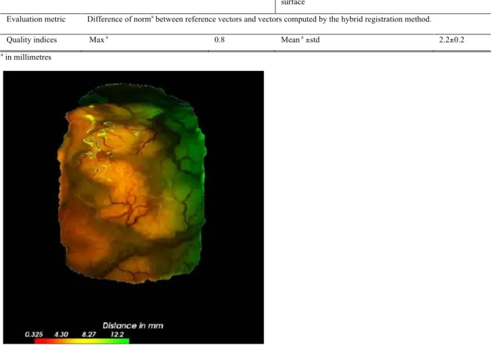
point C and 0.8 mm for point D. For evaluating the surface registration method alone, 3D coordinates of 9 anatomical landmarks in the surface meshes before and after resection were manually identified. These anatomical landmarks were chosen to be different from the tracked ones. The vectors linking these landmarks were compared to those given by the final computed deformation field. The original distance without any registration was 6.2 ± 2.1 mm. For the iterative closest point (ICP) rigid registration, accuracy computed on these 9 extracted points was 5.8 ± 0.9 mm. For the proposed registration method, it was 2.2 ± 0.2 mm. Fig. 5 shows the display of the computed deformation field which was proposed during the intervention to the neurosurgeon.

TABLE II

PERFORMANCE EVALUATION OF THE SURFACE REGISTRATION METHOD ON PATIENT:

DESCRIPTION OF THE EVALUATION PROCEDURE AND RESULTS

Description of

evaluation components

Values for global accuracy evaluation, including localisation

Values for surface meshes registration accuracy evaluation alone

Evaluation data sets 2 surface meshes: before and after resection

Input parameters None

Reference 4 landmarks acquired by the pointer of the

neuronavigation system, recognised by the surgeon

9 points virtually picked on the surface meshes

Error of visual landmarks

recognition

1.9mm Error on surface mesh reconstruction <2 mm

Estimated error

related to the

computation of the

Reference Error of pointer localisation < 0.1mm Error on extraction of a 3D point on the

surface <1 mm

Evaluation metric Difference of norma _{between reference vectors and vectors computed by the hybrid registration method.}

Quality indices Max a _{0.8 Mean} a _{±std 2.2±0.2}

a _{in millimetres}

Figure 5: Visualization of the deformation field on the source surface, acquired just after Dura mater opening and the target surface, after resection. This visualization was 3D, and could be manipulated by the surgeon or medical staff.

IV. DISCUSSION AND CONCLUSION

In this paper, we have introduced a surface registration method, which can be used with any textured cortical surface meshes computed by stereoscopic or laser range approaches. This new surface registration method takes into account both the static

surface meshes and the video flow between these meshes allowing a higher temporal resolution.

The aim of this method was to be able to address the different aspects of complexity encountered in the images all along the surgical procedure. The results of the performance evaluation of this method mainly showed its feasibility in clinical conditions. The global method, including stereoscopic reconstruction and surface registration, had a precision around 2 millimeters, which was the usual rigid registration error of the neuronavigation system before deformations. The video tracker evaluation on different clinical data sets has shown that in sequences without movement of the microscope, the tracking method was sufficiently robust. However, results were described for one patient and one phantom only. These first results are very promising but more clinical cases are needed to prove the robustness of the proposed method and to automatically chose the dynamic model to be used and the parameters α and β.

Another main limitation of our work is the limited dynamic models used, implying the constraint of unchanging zoom and focus settings of the microscope. Future work will consist of defining non-linear models that depend on the surgical step [31] and on tracked modifications of microscope settings.

Other works previously proposed the use of intensity for non-rigid organs surface registration. Sinha et al. [11] used an intensity-based algorithm using mutual information (MI) to register pre operative segmented cortex, which was expressed as a textured point cloud by using ray casting, and a laser range scanning associated with a video camera. Images from video cameras are subject to occlusions by bleeding or tools in the surgical FOV, especially during and after resection. Therefore, MI may not be the most relevant solution in this case. Nakajima et al. [10]have previously proposed the use of cortical vessels for cortical surface registration. The vessels were used as anatomical landmarks, but their intraoperative position was manually defined using the neuronavigation system. In [12], a Euclidean distance-based ICP has been shown to give some good results for brain deformation tracking. However in our clinical case, ICP was not sufficient. The reason is that the different information, which are used by these different algorithms, may be relevant in certain cases but not for other. This was also shown in [26], where the authors compared in an objective way different registration methods, and observed that the methods performed differently according to the patient and the particular clinical case. This shows one of the main advantages of our approach: we can adapt to any case, just by modifying the parameters α and ß from equation (4). We hope to be able to automatically define these weighting coefficients according to the surgical step as a future work. The use of the video flow in brain shift estimation is also new and could be extended to other surgery.

In our opinion, the most promising approach for volumetric brain shift quantification should cope with intraoperative information, both volume and surface, and with modeling of the brain shift phenomenon [2], [35]. Existing 3D imaging devices will certainly give more reliable information regarding the volume deformation. However, their temporal resolution is inferior to the resolution allowed to our approach, since our approach is totally non invasive and does not require any change in the surgical procedure. Combining our surface approach with a volume imaging technique will allow benefiting from the advantages of both methods. The added value of IGNS without correction of deformation has been demonstrated compared to traditional neurosurgery in terms of intervention time and cost per patient [36]. Brain deformation correction should not reduce these advantages with longer interventions due to the use of costly and cumbersome intraoperative imaging devices. Methods of surface registration using the surgical microscope video flow would then be part of the global brain shift correction framework.

ACKNOWLEDGMENT

The authors would like to thank Dr. Elise Arnaud for fruitful discussions about the video tracking, and the reviewers for their very valuable remarks.

REFERENCES

[1] P. Grunert, K. Darabi, J. Espinosa, and R. Filippi. “Computer-aided navigation in neurosurgery”. Neurosurg. Rev., vol. 26, pp. 73–99, May 2003.

[2] J. Cohen-Adad, P. Paul, X. Morandi, and P. Jannin. “Knowledge modeling in image guided neurosurgery: application in understanding intraoperative brain shift,” in Proc. of SPIE – Volume 6141 Medical Imaging 2006: Visualization, Image-Guided Procedures, and Display, San Diego, 2006, pp. 709–716. [3] T. Hartkens et al., “Measurement and analysis of brain deformation during neurosurgery,” IEEE Trans. Med. Imaging, vol. 22, pp. 82–92, Jan. 2003. [4] M. M. J. Letteboer, P. W. A. Willems, M. A. Viergever, and W. J. Niessen, “Brain shift estimation in image-guided neurosurgery using 3-D ultrasound,”

IEEE Trans. Biomed Eng, vol. 52, pp. 268–276, Feb. 2005.

[5] A. P. King, et al., “Bayesian estimation of intra-operative deformation for image-guided surgery using 3-D ultrasound,” in Proceedings of MICCAI’00,

Lecture Notes in Computer Science 1935, Pittsburg, PA, 2000, pp. 588–97.

[6] R. M. Comeau, A. F. Sadikot, A. Fenster, and T. M. Peters, “Intraoperative ultrasound for guidance and tissue shift correction in image-guided neurosurgery,” Med. Phys., vol. 27, pp. 787–800, Apr. 2000.

[7] T. A. N. Hernes, et al., “Computer-assisted 3D ultrasound-guided neurosurgery: technological contributions, including multimodal registration and advanced display, demonstrating future perspectives,” Int. J. Med. Robot., vol. 2, pp. 45–59, Mar. 2006.

[8] X. Pennec, P. Cachier, and N. Ayache, “Tracking brain deformations in time sequences of 3D US images,” Pattern Recognition Letters. Special issue:

Ultrasonic Image Processing and Analysis, vol. 24, pp. 801–813, Feb. 2003.

[9] M. I. Miga, T. K. Sinha, D. M. Cash, R. L. Galoway, and R. J. Weil, “Cortical surface registration for image-guided neurosurgery using laser-range scanning,” IEEE Trans. Med. Imaging, vol. 22, pp. 973–985, Aug. 2003.

[10] S. Nakajima, et al., “Use of cortical surface vessel registration for image-guided neurosurgery,” Neurosurgery, vol. 40, pp. 1201–1208, June 1997. [11] T. K. Sinha, et al., “A method to track cortical surface deformations using a laser range scanner,” IEEE Trans. Med. Imaging, vol. 24, pp. 767–781, June

[12] H. Sun, et al., “Cortical surface tracking using a stereoscopic operating microscope,” Neurosurgery. Operative Neurosurgery Supplement, vol. 56, pp. 86– 97, Jan. 2005.

[13] O. Skrinjar, A. Nabavi, and J. Duncan, “Model-driven brain shift compensation,” Med. Image Anal., vol. 6, pp. 361–373, Dec. 2002.

[14] D. W. Roberts, et al., “Intraoperatively updated neuroimaging using brain modeling and sparse data,” Neurosurgery, vol. 45, pp. 1199–1207, Nov. 1999. [15] O. Clatz, et al., “Robust non rigid registration to capture brain shift from intraoperative MRI,” IEEE Trans. Med. Imaging, vol. 24, pp. 1417–1427, Nov.

2005.

[16] A. Nabavi, et al., “Serial intraoperative MR imaging of brain shift,” Neurosurgery, vol. 48, pp. 787–798, Apr. 2001.

[17] C. Nimsky, et al., “Quantification of, visualization of, and compensation for brain shift using intraoperative magnetic resonance imaging,” Neurosurgery, vol. 47, pp. 1070–1079, Nov. 2000.

[18] A. Hagemann, K. Rohr, and H. S. Stiehl, “Coupling of fluid and elastic models for biomechanical simulations of brain deformations using FEM,” Med.

Image Anal., vol. 6, pp. 375–388, Dec. 2002.

[19] K. E. Lunn, et al., “Assimilating intraoperative data with brain shift modeling using the adjoint equations,” Med. Image Anal., vol. 9, pp. 281–293, June 2005.

[20] M. I. Miga, et al., “Modeling of retraction and resection for intraoperative updating of images,” Neurosurgery, vol. 49, pp. 75–85, July 2001.

[21] M. I. Miga, T. K. Sinha, and D. M. Cash, “Techniques to correct for soft tissue deformations during image-guided brain surgery,” In Biomechanics Applied

to Computer Assisted Surgery, 1st ed., Y. Payan, Ed., Trevendium, India: Research Signpost, 2005, pp. 153–177.

[22] C. Davatzikos, D. Shen, M. Ashraf, and S. K. Kyriacou, “A framework for predictive modeling of anatomical deformation,” IEEE Trans. Med. Imaging, vol. 20, pp. 836–843, Aug. 2001.

[23] P. Jannin, et al., “Integration of sulcal and functional information for multimodal neuronavigation,” J. Neurosurg., vol. 96, pp. 713–723, Apr. 2002. [24] P. Dumpuri, R. C. Thompson, B. M. Dawant, A. Cao, and M. I. Miga, “An atlas-based method to compensate for brain shift: preliminary results,” Med.

Image Anal., vol. 11, pp. 128–145, Apr. 2007.

[25] P. Paul, O. J. Fleig, and P. Jannin, “Augmented virtuality based on stereoscopic reconstruction in multimodal image-guided neurosurgery: methods and performance evaluation,” IEEE Trans. Med. Imaging, vol. 24, pp. 1500–1511, Nov. 2005.

[26] A. Cao, et al., “Laser range scanning for image-guided neurosurgery: investigation of image-to-physical space registrations,” Med. Phys., vol. 35, pp. 1593– 1605, Apr. 2008.

[27] C. Harris and M. Stephens, “A combined corner and edge detector,” in Proc. of the 4th Alvey Vision Conference, Manchester, UK, 1988, pp. 147–151. [28] E. Arnaud, E. Memin, and B. Cernuschi-Fras, “Conditional filters for image sequence-based tracking - application to point tracking,” IEEE Trans. on

Image Processing, vol. 14, pp. 63–79, Jan. 2005.

[29] B. D. O. Anderson and J. B. Moore. Optimal Filtering. Englewood Cliffs, NJ: Prentice Hall, 1979.

[30] F. Bookstein, “Principal warps: thin-plate splines and the decomposition of deformations,” IEEE Trans. on Pattern Analysis and Machine Intelligence, vol. 11, pp. 567–585, June 1989.

[31] P. Jannin, M. Raimbault, X. Morandi, L. Riffaud, and B. Gibaud, “Model of surgical procedures for multimodal image-guided surgery,” Comput. Aided

Surg., vol. 8, pp. 98–106, Mar. 2003.

[32] W. H. Press, S. A. Teukolsky, W. T. Vetterling, and B. P. Flannery, Numerical Recipes in C - The Art of Scientific Computing. Cambridge, UK: University Press, 1992, pp. 683–688.

[33] P. Jannin, C. Grova, and C.R. Maurer, “Model for defining and reporting reference-based validation protocols in medical image processing,” Int. Journal of

Computer Assisted Radiology and Surgery, vol. 1, pp. 63–73, Aug. 2006.

[34] I. Reinertsen and D. L. Collins, “A realistic phantom for brain-shift simulation,” Med. Phys., vol. 33, pp. 3234–3240, Sept. 2006.

[35] C Barillot, et al., “Image guidance in neurosurgical procedures, the Visages point of view,” in IEEE International Symposium on Biomedical Imaging:

From Nano to Macro ISBI’07, Washington DC, 2007, pp. 1056–1059.

[36] T. Paleologos, O. Wadley, N. Kitchen, and C. Thomas, “Clinical utility and cost-effectiveness of interactive image-guided craniotomy: clinical comparison between conventional and image-guided meningioma surgery,” Neurosurgery, vol. 47, pp. 40–48, July 2000.