AUTOMATIC PLACEMENT OF THE HUMAN HEAD THANKS TO ERGONOMIC AND VISUAL CONSTRAINTS

HAL Id: hal-01160624

https://hal.archives-ouvertes.fr/hal-01160624

Submitted on 18 Jun 2015

HAL is a multi-disciplinary open access

archive for the deposit and dissemination of

sci-entific research documents, whether they are

pub-lished or not. The documents may come from

teaching and research institutions in France or

abroad, or from public or private research centers.

L’archive ouverte pluridisciplinaire HAL, est

destinée au dépôt et à la diffusion de documents

scientifiques de niveau recherche, publiés ou non,

émanant des établissements d’enseignement et de

recherche français ou étrangers, des laboratoires

publics ou privés.

AUTOMATIC PLACEMENT OF THE HUMAN

HEAD THANKS TO ERGONOMIC AND VISUAL

CONSTRAINTS

Bilal Boualem, Damien Chablat, Abdelhak Moussaoui

To cite this version:

Bilal Boualem, Damien Chablat, Abdelhak Moussaoui. AUTOMATIC PLACEMENT OF THE

HU-MAN HEAD THANKS TO ERGONOMIC AND VISUAL CONSTRAINTS. Proceedings of the ASME

2015 International Design Engineering Technical Conferences & Computers and Information in

Engi-neering Conference, Aug 2015, Boston, United States. �hal-01160624�

Proceedings of the ASME 2015 International Design Engineering Technical Conferences & Computers and Information in Engineering Conference

IDETC/CIE 2015 August 2-5, 2015, Boston, Massachusetts, USA

DETC2015-46153

DRAFT: AUTOMATIC PLACEMENT OF THE HUMAN HEAD THANKS TO

ERGONOMIC AND VISUAL CONSTRAINTS

Bilal BOUALEM University of Tlemcen Tlemcen, ALGERIA Institut de Recherche en Communication et Cybernétique de Nantes, UMR CNRS 6597 bilal.boualem@ec-nantes.fr Damien CHABLAT Institut de Recherche en Communication et Cybernétique de Nantes, UMR CNRS 6597, Nantes, France Damien.Chablat@cnrs.fr Abdelhak MOUSSAOUI University of Tlemcen Tlemcen, ALGERIA University of Lorraine Metz, FRANCE abdelhak.moussaoui@univ-lorraine.fr ABSTRACT

This article aims to create automatic placement and trajectory generation for the head and the eyes of a virtual mannequin. This feature allows the engineer using off-line programming software of mannequin to quickly verify the usability and accessibility of a visual task. An inverse kinematic model is developed taking into account the joint limits of the neck and the eyes as well as interference between the field of view and the environmental objects. This model uses the kinematic redundancy mechanism: the head and eyes. The resolution algorithm is presented in a planar case for educational reasons and in a spatial case.

INTRODUCTION

The need for designers, builders and manufacturers of tools that allow the study of the interaction of the humans with their environments and the designed products has prompted researchers to develop tools for the study of accessibility.

Computer tools (CATIA, SolidWorks, NX, PCT CREO, SANTOS, etc.); using virtual reality; have emerged to meet this demand. These tools are used to evaluate the mechanical and visual capabilities of the human to accomplish a task (Driving a car, using the computer keyboard, dial a phone number). However, there are a lot of drawbacks in these tools. For example, in the mannequin simulation, we are able to look at the hand but without taking into account the distance between the hand and the eyes and the size of the object.

In the literature, we find different approaches to compute the head motion to get a visible target. In [1], the author proposes an approach based on a multi-agent system that

distributes the computation of the posture of the mannequin over several elementary agents (an agent to move the mannequin, an agent for the detection of collisions, an agent to keep the target visible, etc.). Another approach presented by T. Marler in [2] where he considers the vision as a criterion among several criteria to be satisfied. This is known as a multi-objective optimization problem. There are several methods and algorithms to solve it [3]. The works cited above define a cone of vision that describes the field of view of the eyes. An object is considered as visible if it belongs to this cone and no obstacle interferes between the object and the eyes. The distance between the eyes and the object, the size of the object are not considered.

In our approach, we consider the eyes as a part of the human upper body model, in other words, neck, head, eyes and vector of sight are considered as an additional end of the body of the mannequin. This end of the body is modeled according to the capabilities of the eyes.

The visibility problem becomes an inverse kinematics problem. We use the method described by Aristido in [4] to solve it. We improve this method to detect and avoid obstacles present inside the environment.

HUMAN UPPER BODY MODELING

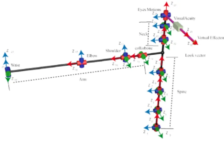
In this section, we describe the geometrical model of the human upper body. We start by the presentation of the model proposed by T. Marler in [2]. The author proposes a model with 26 degrees of freedom (dof) as it is shown in the Fig. 1: 12 dof are used to model the spine, 2 dof for the collarbone and 3 for the shoulder, 2 for the elbow, 2 for the wrist and 5 dof for the

neck. We notice that all joints are rotational. We use this model because it gives a realistic posture of the mannequin with a reduced computational cost.

Fig. 1: T. Marler’s Human upper body Model

In our approach, we consider the eye features as an extension of the human upper body model. In other words, the eyes features are an additional joints and links added to the neck model.

The ability for human to see an object is related to the eyes features (Eyes motion, field of view, and visual acuity) and the environment (lighting, obstacle between the eyes and the object). In this work, we are not interested by the lighting conditions.

Visual acuity

The visual acuity is the ability to distinguish the details of the object. According to this report [5], there are several techniques to assess the visual acuity. The most used are the Snellen’s chart described by I. Bailey in [6]. The technique is based on the ability of the person to read a letter of a size S from a certain distance D. The Figure 2, shows the Snellen principle, where S is the height of the letter (or object) and D is the distance between the eyes and the object, α is the angular size of the letter in minutes of arc (1 minute of arc = π/10800 radians).

Fig. 2: Snellen principle

The Fig. 3 shows an example of a letter used to assess the visual acuity. The letter is composed of three black zones and two white zones. A human can read this letter if he can distinguish every zone.

Fig. 3: Snellen’s letter

The size of every zone (α/5) is called the minimum angle of resolution (MAR). Using the MAR, we can get the maximum distance to see an object.

(

)

where MAR is the MAR for far vison. _far

In the same way, we use the MAR for the near vision to compute the minimum distance [7].

(

)

where MAR_near is the MAR for near vison.

The object must be at a distance DÎ êé_ëD_min, D_maxù_{úû to be} visible. This can be modelled as a prismatic joint that gives the ability to vary the length of the virtual link (the look vector). The field of view

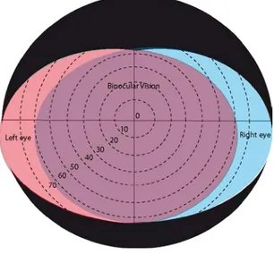
The field of view is the visible space for a motionless eyes and head. According to Parker [8], the field of view is the union of the visible spaces of the two eyes, as it is shown in the Fig. 4. The blue zone represents the right eye and the red zone the left eye. The intersection zone, called the binocular vision. The human solicits both eyes to see.

Fig. 4: Field of view

The visual acuity is at the maximum in the centre zone, called the fovea. The visual acuity drops exponentially when the

object is far from the centre. In [2]. The author proposes a function to compute the deterioration of the acuity visual according to the angle between the eye to target vector and the fovea. It is expressed as:

7| | e

-= θ

e (3)

where θ represents the angle between the eye to target vector and the fovea vector.

Therefore, the problem is to reduce θ. Considering the look vector (fovea) as an virtual link, The application of an inverse kinematics algorithm resolve the problem, if the virtual effector reach the target q =0, if not the algorithm try to close to the target. At this moment, we can check the visibility of the target by reducing the visual acuity using (3). Then we compute the minimal and maximal distance using (1) and (2). Finally, check if the distance eye to target belongs to é_êëD_min, D_maxù_úû.

The eyes movements

The aim of moving the eyes is to enclose the object to the fovea zone.

According to [9] and [10], the eyes movements can be represented using two rotations. The first rotation moves the gaze up and down while the second one moves it right and left. The range of the motion is ±55°.

We can conclude that the eyes behave as a joint with 2 dof. Therefore, to model the eyes movements we add a joint with 2 dof on the top of the neck; this joint orients a virtual link (that represents the look vector) to the target.

The Full model

Figure 5 shows the model of the human upper body considering the eyes features. The eyes are modelled using a prismatic joint representing the visual acuity and a rotational joint with 2 dof to represent the eyes motions.

Fig. 5: The human upper body

Using this approach to model the eyes behaviour, we can define different targets for the hands and the eyes. It is possible,

also, to give more importance to the reachability of the hand or the visibility.

FORMULATION OF THE PROBLEM

Now, the problem is to find the posture of the mannequin that allows to the two arms to reach the targets. The problem is known in the literature as an inverse kinematics problem it can be formulated as:

We assume that the current positions of the effectors are Peff1 and Peff2 and the current orientations are Reff1 = [X eff1, Y eff1,

Z eff1] and Reff2 = [X eff2, Y eff2, Z eff2] (where X eff, Y eff and Z eff are

the unit vectors associated to the effector).

Given a desired positions t1 and t2 and the desired

orientations are Rd1 = [X d1, Y d1, Z d1] and Rd2 = [X d2, Y d2, Z d2].

Find the posture such as: Peff1 = t1

Peff2 = t2

Reff1= Rd1

Reff2= Rd2

INVERSE KINEMATICS ALGORITHM

The cyclic coordinate descent (CCD) algorithm, described in [11], used in many fields to solve the IK problem (i.e compute the posture of an articulated body), this method considered as a fast and robust algorithm but the posture obtained is unrealistic making it not adapted for animating human.

A. Aristidou proposes an algorithm, called Forward and backward invers kinematics (FABRIK) in [4], to solve IK problem. This algorithm is faster, robust and offers a realistic posture. In addition, the geometrical aspect of the algorithm makes the detection and the avoidance of obstacles simpler. These advantages justify our choice to use this algorithm.

In this section, we describe the Forward and backward invers kinematics algorithm, developed by A. Aristidou. This algorithm is very fast, and the solution obtained is realistic, compared to other IK algorithms (CCD).

We take the example of the manipulator, shown in Fig. 6 to explain FABRIK algorithm. The manipulator contains four joints connected by four links. We note Pi the Cartesian position

of the joint “i” and di the length of the link “i”. We can

Fig. 6: An example of a planar manipulator

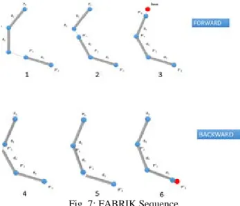
 Unconstrained case: FABRIK method is an iterative algorithm that solves the IK problem, each iteration of the algorithm divided on two steps:

On the first loop, called forward step, we place the effector on the target position then we move the n-1th joint on the line linking the effector and Pn-1, We note the new position

P’n-1. P’n-1 is at dn-1 of the effector as it is shown in the

Figure 7-1. In the same way, we move the next joints until the base (P0), as shown in Fig. 7-2 and 7-3.

However, in the backward step, we start by placing the base (first joint of the manipulator) on its original position, and then we move the joint 2 on the line connecting the original position of the base and the P’2,we place P2 at d1 from the

base. Repeating the iteration (Forward and backward steps), cancels the error between the effector and the target.

Fig. 7: FABRIK Sequence

The algorithm is fast, simple to implement and the posture obtained is more realistic then the other IK method. This makes this algorithm the best compromise in the unconstrained case.

Fig. 8: Constrained FABRIK

 Constrained case: In this case, the constraints represent the joint limits; they are defined on the joint space. It is hard to consider the joints limits in the compute steps because of the difference between the Cartesian space and the joints space. A. Aristidou proposes a method to respect joints limits. The goal of this method is to check if the computed position of the joint i (on the forward or backward loop) P’i is in the

reachable set of the joint else take the closest point to P’i.

The Figure 8 shows a planar example to check if the position P’i respecting the joint limits (θli, θui). First, we

must define the reachable set. So, we starts by compute the projection, noted O, of the point P’i on the extension of the

segment Pi+1 Pi+2 (red line) as shown in the Figure 8. Then

we compute q₁=|| O P ||- _i-1 tan( )q_iu and

2 || O P ||1 ( )

l i tan i

q = - _- q , then we check if P’i is in the

segment [O q O- ₂, ,q₁], then keep P’i . Else we choose the

nearest position to P’i (new_ P’i)as it is shown in the Figure

8. In the 3D case, A. Aristidou defines the reachable set as an ellipse centred on O and q₁, andq₂ q₃ ,q₄ are major and minor radius.

This method work perfectly especially when the joints limits are lower than 𝞹𝞹/2, but it is unstable when the boundaries are equal to 𝞹𝞹/2; this instability is due to the tangent function.

To respect the joints limits, it is necessary to find a transformation that allows the transition from the joint space to the Cartesian space or the inverse (i.e from the Cartesian space to the joint space). The author chosen to use tangent function to do the transformation but this function presents singularity at π/2 that make the algorithm unstable near this singularity. Therefore, we need a reliable and a fast algorithm to respect joint limits.

In the next section, we propose a new reliable method to respect the joints limits.

The Figure 9 shows a manipulator in 3D space. This manipulator is composed of four rotational joints. We callX_i the unit vector associated to the extension of the segment [Pi-1

Pi] (or [Pi+1 Pi] in the forward step) illustrated by the red vector

in the Figure 9. Y Z_i, _i (blue and green vectors ) are a units vectors belonging to the plan perpendicular to the vectorX_ias it is shown in the Figure 9. We call system “i”, the frame composed of (X_i,Y Z_i, _i).

Fig. 9: An articulated body in 3D Formulation of the problem

The problem can be defined as:

Given P’i the new position of the joint “i” computed by

FABRIK, and [θli, θui] is the lower and the upper limits of the

joints “i”. Considering a joint limit restricts the set of reachable points (SRP).

The problem is to check if the point P’i belongs in the SRP

to the joint “i”. Then keep P’i.

Else take the closest point to P’i from SRP.

Constrained FABRIK

To apply the joint limits to the joint “i”, we divide into two problems, the first is the orientation problem; it consists to orients the Y Z_i, _i vectors. The second is the position problem. It consists to check if the new position of the joint “i” P'_i respects the joint constraints.

Assume we are in the first step (i.e forward loop), to apply the joint limits, we start by orienting (Xi, Yi, Zi) such that the

segment Pi+1Pi and Xi become collinear. For this, we need to

find the rotor expressing the rotation between the Xi vector and

the segment Pi+1Pi. We use the quaternion to represent the

rotation around a vector, because it is simpler, faster and more efficient than the rotation matrix, according to [12].

To find the quaternion we need to find the rotation vector V and the angle α between the two vectors, Xi and Pi+1Pi. V is the

normal vector perpendicular to the plane (Xi, Pi+1Pi). We note

that the use of P’i or Pi to compute the vector V and the angle α

is the same because P’i, Pi and Pi+1 are in the same line.

1 1 i i i i P P V Xi P P , , æ _ö÷ ç _÷ ç _÷ ç _÷ ç -= ççè ø Ù - ÷÷

and the angle can be found using the dot product as follow: 1 1 cos i i i i P P ar Xi P P a , , æ _ö÷ ç _÷ ç _÷ ç æ _{- ö÷} ç _÷ ç _÷ = ç_ç · _÷÷ ç - ÷÷ çè çççè ÷÷÷øø

Now, we define the quaternion such as

; 2 2 Q ê_êécosçç_ççæ öa÷_÷÷÷ sin_çç_ççæ öa÷_÷÷_÷V_úùú è ø è êë û = ø ú

Using the quaternion, we compute the new vectors X’i,

Y’i and Z’i by rotating each vector using the quaternion as

follow: 1 ’_i Y ₌QV Q -Where Q-1 =Q’ / Q , ’ ; 2 2 Q =é_êêcosæ öç_çça_÷÷÷÷ sinæ ö_ççça÷_÷÷_÷V_úúù ç ç è ø è êë û -ø ú is the conjugate of Q.

The multiplication of two quaternions p= é_êëp p p p_{1 2 3 4}ù_úû and q= é_êëq q q q_{1 2 3 4}ù_{úû is} 1 1 2 2 3 3 4 4 1 2 2 1 3 4 4 3 1 3 2 4 3 1 4 2 1 4 2 3 3 2 4 1 pq p q p q p q p q p q p q p q p q p q p q p q p q p q p q p q p q é _{- - -} ù ê ú ê _{, , -} ú ê ú = ê _{- , ,} ú ê ú ê _{, - ,} ú ê ú ë û

The orientation constraints

In the forward step, Given the two systems: “i+1” (Xi+1,

Yi+1, Zi+1 ) associated to the joint “i+1” and “i” (Xi, Yi, Zi )

associated to the joint “i”.

If Xi and Xi+1 are collinear then the orientation of the system

“i” is the angle between (Yi and Yi+1) or (Zi and Zi+1).

So, considering the system “i+1” is fixed, the problem is to find the angle q₁ between the vectors (Yi and Yi+1) or (Zi and

Zi+1).q1 must respects the orientation: 1

l u i i

q <q <q

If Xi and Xi+1 are not collinear, we need to express the rotor

the orientation angle. It is possible to use a decomposition to the Euler angles as described in [12].

To compute the rotor, we start by projecting Xi on the (Xi+1

Yi+1) and (Xi+1 Zi+1) planes, using the algorithm presented on

[13]. Using the cross and the dot product it is easy to find the rotations φ and ψ around the axes Yi+1 and Zi+1 to have the

vetors Xi, Xi+1 collinear.

The rotation angle θ1 represents the angle between (Yi and

Yi+1) or (Zi and Zi+1) as long as the two vectors Xi, Xi+1 are

collinear (we must rotate Yi to be in the Yi+1 Zi+1 plane).

Therefore, using the quaternion, we rotate Yi around the

vectors Yi+1 and Zi+1 to find Y’i, the rotation result of Yi. This

transformation allows us to compute the angle:

(

)

1 arcosY Yi i 1

q = ¢· _,

Now, we can check if 1

l u i i

q <q <q

If θ1 ∈ [θli, θui] then keep θ1. However, if θ1 ∉ [θli, θui],

we take the closest boundary θli, θui. Then we compute the new

Yi andZi by rotate Yi+1 andZi+1 around Xi+1, Yi+1 andZi+1 by

new_θ, ψ and φ respectively. Algorithm

Inputs: [Xi, Yi, Zi], [Xi+1, Yi+1, Zi+1] and θli, θui

Outputs: [ Xi, Yi, Zi]

- Compute φ and ψ by projecting Xi on the Xi+1Yi+1 and

Xi+1Zi+1 plans

- Q1= [cos (ψ /2); sin (ψ /2) Yi+1]

- Q2= [cos (φ /2); sin (φ /2) Zi+1]

- Y’i = Q1*Q2 * Yi * Q1-1* Q2-1

- θ1 = acos (<Y’i , Yi+1>)

- If θ1 ∈ [θ l i, θui] then keep θ1. - Else if (θ1 - θli)2<( θ1-θui)2 then new_θ1 = θli Else new_θ1 = θ u i

- Q1= [cos (ψ /2); sin (ψ /2) Yi+1]

- Q2= [cos (φ /2); sin (φ /2) Zi+1]

- Q2= [cos (new_θ1 /2); sin (new_θ1 /2) Xi+1]

- Q= Q1*Q2 * Q2

- Yi =Q * Yi+1 * Q-1

- Zi = Q * Zi+1 * Q -1

The position constraints

P’i is a combination of the rotation around Xi, Yi and Zi

vectors, in the previous section we described a method for computing the orientation of Yi and Zi vectors, Now, we are

interested in calculating the rotation angles around Yi and Zi

vectors. Instead of considering the 3D Problem, we divide it into two 2D problems. This will simplify it.

We note that a rotation around Yi axis only, generates a

variation of P’i in the (Xi Zi) planar and a rotation around Zi axis

only generates a variation of P’i in the (Xi Yi) planar. Therefore,

to find the rotation angles, we simply project P’i on the two

planes (Xi Yi) and (Xi Zi). We note P’jz, P’jy the projections of P’i

on the XiZi, XiYi planes respectively.

Now, It is possible to find the angles θ2 (between the

segment [P’i+1P’jz] and Xi) and θ3 (between the segment

[P’i+1P’jy], Xi ), using the dot and the cross products.

After that, we can check if

2 2 2 l u q <q <q 3 3 3 l u q <q <q

If θi ∈ [θli, θui] then keep θi. However, if θi ∉ [θli, θui], we

take the closest boundary θli, θui. We note that to check θ2 (the

angle between the segment P’i+1P’jz and Xi axis) we use the

limits applied to the rotation around Yi axis.

We compute the new P’jy P’jz, by using the following

expressions:

(

)

(

)

(

)

’_jy _ ( _ _i _ _i)

P =cos new q cos new q x ,sin new q y

(

)

(

)

(

)

’_jz _ ( _ _i _ _i)

P =cos new q cos new q x ,sin new q z

Now, we need to compute the new position P’i from the

projections P’jy, P’jz. Therefore, P’i is the point of intersection

between the normal vectors of (XiYi) and (XiZi) planes on the

projection point P’jy, P’jz.

Since the points P’i, Pi and Pi+1 are on the same line it is

possible to use P_i directly to check the position constraints without computing the new position P’i. It will be computed at

the end of the position constraint algorithm. Algorithm

Inputs: Pi, Pi+1, [Xi, Yi, Zi], di and θli, θui

Outputs: P’i

- Compute P’jy and P’jz, the projections of Pi on the XiYi

and XiZi plans

- θ2 = acos (<Xi , (P’jz - Pi+1)>/|| (P’jz - Pi+1)||)

- θ3 = acos (<Xi , (P’jy - Pi+1)>/|| (P’jy - Pi+1)||)

- check θli<θ2< θui

θl

i<θ3< θ u

i

- P’jy = cos (new_θ3) (cos (new_θ2) xi + sin (new_θ2) yi)

- P’jz = cos (new_θ2) (cos (new_θ3) xi + sin (new_θ3) zi)

- n1=cross(Xi , Yi)

- n2= cross(Xi , Zi)

- Find new_P’i the intersection between n1 and n2 at P’jy ,

P’jz.

- P’i =di (new_P’i - Pi+1)/|| (new_P’i - Pi+1) ||

The full algorithm

Assuming, we have n dof manipulator and Pi and [Xi, Yi, Zi]

are the positions and the coordinates systems associated to the joint “i”, we pose t and Rt = [Xt, Yt, Zt] the desired position and

The consideration of the joint limits will affect the speed of the algorithm, but we can simplify the algorithm. The full algorithm becomes Algorithm Inputs: t, Rt, Pi, [Xi, Yi, Zi] and θli, θui Outputs: Pi, [Xi, Yi, Zi] - ε = 0.1 - di = || Pi - Pi+1|| i=1,…,n - if || Pi - Pi+1||>d1 + d2 +…+ dn-1 then t is unreachable - else

- b =P1 % keep the base position

- [ Xbase, Ybase, Zbase ] = [X1, Y1, Z1 ]% keep the units

vectors of the base (joint 1)

- error=|| t– Pn|| Compute the error between the target

t and the effector - while error > ε

% forward step Pn = t

[Xn, Yn, Zn]= Rt

For i=n-1,…,1

% call the position constraint function

Pi =contrainte_position(Pi, Pi+1, [Xi+1, Yi+1,

Zi+1], [θli θui])

%orienting the system Xt = Pi+1 – Pi/|| Pi+1 – Pi||

Angle = acos(<Xi , Xt >)

Axis = cross(Xi , Xt )

[Xi, Yi, Zi]=rotate([Xi, Yi, Zi], Angle, Axis)

%Orientation limits of the next coordinate system

[Xi, Yi, Zi] =constaint_orientation([Xi, Yi, Zi],

[Xi+1, Yi+1, Zi+1], [θ l i θ u i]) End % backward step P1 = b

[X1, Y1, Z1 ]=[ Xbase, Ybase, Zbase ]

For i=1,…,n-1

Pi+1 =contrainte_position(Pi+1, Pi, [Xi+1, Yi+1,

Zi+1], [θli θui])

Xt = Pi+1 – Pi/|| Pi+1 – Pi||

Angle = acos(<Xi+1 , Xt >)

Axis = cross(Xi+1 , Xt )

[Xi+1, Yi+1, Zi+1]=rotate([Xi+1, Yi+1, Zi+1], Angle,

Axis)

[Xi+1, Yi+1, Zi+1] =constaint_orientation([Xi+1,

Yi+1, Zi+1], [Xi, Yi, Zi], [θli θui])

End

- error=|| t– Pn||

- End

Spatial Constraints (Collision-free)

The mannequin had to avoid the collision with the objects present in the virtual environment while doing a task. We need to simplify the geometry of the objects to reduce the computations. There are lot of techniques of the simplification of the geometry used in virtual reality; the most used is the minimal enclosing box described in [14]. This technique simplifies the geometry of an object to a box. Another technique, presented by Hariri in [15], decomposes the object to several simple objects (spheres, planes, boxes), this technique is more accurate.

The links of the mannequin are considered as segments. At each iteration “i” after computing the new position of the articulation P’i (in the forward loop); we check the

intersection between the segment [Pi+1, P’i] (in the forward

loop) and the box; the existence of the intersection is the proof of a collision between the link and the object. The new position

new_P’i (that avoid the collision) need to guarantee three

conditions:

1. No intersection between [Pi+1; new_P’i] and the box

This condition allows to avoid the obstacle

2. No intersection between [new_P’i, Pi-1] and the box: This

condition guarantees the existence of at least one solution in the next iteration. In the unconstrained case (without orientation and position constraints), this condition avoid to check the collision in the next iteration.

3. new_P’i is the nearest position of the joint “i” to P’i

satisfying the previous conditions.

To find new_P’i, we discretize the SRP of the joint “i” (the

positions of the joint “i” respecting the position constraints) as shown in Fig 10.

Among this set, the green arc defines the positions respecting the conditions (1 and 2); the pink part defines the positions respecting the first condition only and the red part defines the positions respecting any conditions from (1 and 2).

We choose the nearest position to P’i that satisfies the

conditions described above.

In constrained case (with orientation and position constraints), if there is any position of SRP that satisfied the first condition, we vary the previous joint to find the position that satisfy the conditions.

Fig. 10: Collision-free Approach

RESULTS AND DISCUSSION

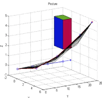
To test the inverse kinematics algorithm considering joints and spatial constraints, we use an articulated body model with four rotational joints allowing a 3 DOF constrained motion. The articulated body is described in the Fig. 11.

Figure 11 shows an obstacle in the middle of the scene. The initial posture of the articulated body is shown in blue the target is the red “+ symbol”. Figure 11 shows the evolution of the posture from the initial posture to the final one.

Fig. 11: Collision-free FABRIK results

We notice that the algorithm choose the best way to avoid the obstacle from the first posture. The final posture satisfies the orientation, position and the spatial constraints.

The error evolution is shown in the Figure 12. After 18 iterations, the algorithm converges to the solution.

Fig. 12: Error evolution

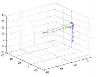
Figure 13 shows the initial posture of the human upper body. The red “+ symbol” define the target of the eyes and the hand. The blue articulated body represents the spine this part is shared between the left arm (red) and the neck and eyes features part (green).

Fig. 13: initial posture

Applying the algorithm, we get the result shown in the Figure 14. We can notice that the vision influences the posture and specially the head position.

The algorithm is simple to implement and the posture is realistic. The speed of the algorithm depends essentially to the size of the obstacles and the technique chosen to simplify the geometry. These advantages are making this algorithm interesting in the virtual reality field.

Fig. 14: Final posture

CONCLUSIONS

In this paper, we presented a new approach to model a human vision. It is based on the features of the eyes (Vision field, Visual acuity, eyes motion and no interference with obstacles). We consider the look vector as an additional end of the human model.

This modelling allows us to formulate the visibility problem as a classic IK problem for a multi arms articulated body.

We used an improved FABRIK algorithm to solve the IK problem for multi arms articulated body and we presented an algorithm to avoid the collision with obstacles. After detecting a collision between a link and an object, we try to find a position that avoids the collision by analysing the joint space.

For future works, we project to use different techniques to analyse the whole space [16] and considering a global solution of the IK problem avoiding collision.

ACKNOWLEDGMENTS

The work presented in this paper was partially funded by the Erasmus Mundus Active.

REFERENCES

[1] D. Chablat, P. Chedmail, and L. Pino, “A distributed approach for access and visibility task under ergonomic constraints with a manikin in a virtual reality environment,” in 10th IEEE International Workshop on

Robot and Human Interactive Communication, 2001. Proceedings, 2001, pp. 32–37.

[2] T. Marler, K. Farrell, J. Kim, S. Rahmatalla, and K. Abdel-Malek, “Vision Performance Measures for Optimization-Based Posture Prediction,” SAE International, Warrendale, PA, SAE Technical Paper 2006-01-2334, Jul. 2006.

[3] R. T. Marler and J. S. Arora, “Survey of multi-objective optimization methods for engineering,” Struct.

Multidiscip. Optim., vol. 26, no. 6, pp. 369–395, Mar.

2004.

[4] A. Aristidou and J. Lasenby, “FABRIK: A fast, iterative solver for the Inverse Kinematics problem,” Graph.

Models, vol. 73, no. 5, pp. 243–260, Sep. 2011.

[5] “Recommended stardard procedures for the clinical measurement and specification of visual acuity. Report of working group 39. Committee on vision. Assembly of Behavioral and Social Sciences, National Research Council, National Academy of Sciences, Washington, D.C,” Adv. Ophthalmol. Fortschritte Augenheilkd. Prog.

En Ophtalmol., vol. 41, pp. 103–148, 1980.

[6] I. L. Bailey and J. E. Lovie, “New design principles for visual acuity letter charts,” Am. J. Optom. Physiol. Opt., vol. 53, no. 11, pp. 740–745, Nov. 1976.

[7] I. L. Bailey and J. E. Lovie, “The design and use of a new near-vision chart,” Am. J. Optom. Physiol. Opt., vol. 57, no. 6, pp. 378–387, Jun. 1980.

[8] J. F. Parker Jr. and V. R. West, “Bioastronautics Data Book: Second Edition. NASA SP-3006.,” NASA Spec.

Publ., vol. 3006, 1973.

[9] H. Misslisch, D. Tweed, and T. Vilis, “Neural Constraints on Eye Motion in Human Eye-Head Saccades,” J.

Neurophysiol., vol. 79, no. 2, pp. 859–869, Feb. 1998.

[10] D. Guitton and M. Volle, “Gaze control in humans: eye-head coordination during orienting movements to targets within and beyond the oculomotor range,” J.

Neurophysiol., vol. 58, no. 3, pp. 427–459, Sep. 1987.

[11] L.-C. T. Wang and C. C. Chen, “A combined optimization method for solving the inverse kinematics problems of mechanical manipulators,” IEEE Trans. Robot. Autom., vol. 7, no. 4, pp. 489–499, Aug. 1991.

[12] J. B. Kuipers, Quaternions and Rotation Sequences: A

Primer with Applications to Orbits, Aerospace and Virtual Reality. Princeton, N.J.: Princeton University

Press, 2002.

[13] M. de Berg, O. Cheong, M. van Kreveld, and M. Overmars, Computational Geometry: Algorithms and

Applications, Édition: 3rd ed. 2008. Berlin:

Springer-Verlag Berlin and Heidelberg GmbH & Co. K, 2008. [14] J. O’Rourke, “Finding minimal enclosing boxes,” Int. J.

Comput. Inf. Sci., vol. 14, no. 3, pp. 183–199, Jun. 1985.

[15] M. Hariri, “A study of optimization-based predictive dynamics method for digital human modeling,” University of Iowa, 2012.

[16] S. Laine and T. Karras, “Efficient Sparse Voxel Octrees,” in Proceedings of the 2010 ACM SIGGRAPH Symposium

on Interactive 3D Graphics and Games, New York, NY,