HAL Id: hal-01277760
https://hal.archives-ouvertes.fr/hal-01277760
Submitted on 23 Feb 2016HAL is a multi-disciplinary open access archive for the deposit and dissemination of sci-entific research documents, whether they are pub-lished or not. The documents may come from teaching and research institutions in France or abroad, or from public or private research centers.
L’archive ouverte pluridisciplinaire HAL, est destinée au dépôt et à la diffusion de documents scientifiques de niveau recherche, publiés ou non, émanant des établissements d’enseignement et de recherche français ou étrangers, des laboratoires publics ou privés.
Wear analysis of hip explants, dual mobility concept:
Comparison of quantitative and qualitative analyses
Laurianne Imbert, Jean Geringer, Bertrand Boyer, Frédéric Farizon
To cite this version:
Laurianne Imbert, Jean Geringer, Bertrand Boyer, Frédéric Farizon. Wear analysis of hip explants, dual mobility concept: Comparison of quantitative and qualitative analyses. Proceedings of the Institution of Mechanical Engineers, Part J: Journal of Engineering Tribology, SAGE Publications, 2012, 226, pp.838 - 853. �10.1177/1350650112451211�. �hal-01277760�
Wear analysis of hip explants, dual mobility concept:
comparison of quantitative and qualitative analyses
L. Imberta, J. Geringera,c,*, B. Boyerb, F. Farizonb
a
Ecole Nationale Supérieure des Mines, CIS-EMSE, CNRS:UMR5146, LCG, F-42023 Saint-Etienne de Saint-Etienne Tel: +33 477 426 688; geringer@emse.fr
b
Centre d’Orthopédie Traumatologie CHU St Etienne F-42055 St Etienne cedex 2
c
Penn State University, MSE/CEST, 206A Steidle Building, University Park 16802 PA USA Tel: 001 814 954 2225; jag54@psu.edu
Abstract
Total hip replacement (THR) fails mainly because of wear. It is of interest to analyze wear to be able to increase the longevity of the hip implants. One way to achieve it is to use instruments on explants but the most suitable depends on the application. This paper aims at comparing several methods of surface analysis in the particular application of wear determination in a series of dual mobility explants. Wear measurement could help understand the wear mechanism only partially known. A CMM, Coordinate Measuring Machine, is used to get 3D points representing the explants, then Pro/Engineer® and Matlab® are used to calculate wear. A mechanical (SOMICRONIC®) and an optical profilometer (Bruker nanoscope Wyko® NT 9100, ex. Veeco) are used to access roughness parameters. The comparisons of the two software showed similar results for wear calculation except in a few cases where differences are due to the theoretical volumes calculation. The comparison of the two profiling techniques resulted in similar results particularly for Sa and Sdr. The comparison of the results showed that wear is present for four explants; it is relevant with the observed characteristics. The mechanical profilometer showed better accuracy than the optical one which enable to conclude that it must not be neglected for that particular application, even if measurements need more time.
Keywords: Total hip replacement; explants; dual mobility concept; wear measurements; surface roughness.
1. Introduction
The hip joint, like every other joints, can suffer from a disease or a fracture and might need to be replaced. That surgery is one of the most common performed nowadays but it is likely to occur several times in a lifetime since a total hip replacement (THR) lasts 15-20 years at most.
The most common cause of premature failure of implanted joints is aseptic loosening, accounting for 75% of revision operations. Aseptic loosening can be attributed to macrophage (immune system) response to particulate debris generated by wear of the components, and bone resorption due to stress shielding after prosthesis implantation [1].
Wear of hip replacement can be studied by several ways like numerical simulation [2-5], tests performed on simulators [1,6-8] or explants analysis [1,9-11]. When analyzing explants, i.e. implants removed from patients, one needs to look at the surface to get information on wear mechanisms. Quantitative and qualitative information can be obtained using appropriate instruments. For instance Geringer et al. used a coordinate measuring machine (CMM) to calculate wear volumes and a mechanical profilometer to assess the surface roughness on a series of twelve dual mobility explants and a blank cup [9].
Quantification of wear can be carried out by roundness measurements or gravimetric methods. Gravimetric testing consists in weighing the implant before and after being used. This technique has some limits since the surfaces have been proved to change, for instance protein absorption may occur [12]. Besides it seems possible only for in vitro studies given the initial implant weight is not known. L. Blunt et al. seemed to think that a geometric method like CMM could overcome several problems linked to the gravimetric technique like the surface absorption [1]. However the initial data are often unavailable as well but they overcame it by using a similar implant or the no-wear zones as reference [1]. The principle of this technique is to get the coordinates of many points on the implant surface. Morris et al. validated the use of a CMM for implant analysis and suggested it to be applicable for explants analysis as well. Moreover they found a strong correlation between the CMM method and the gravimetric method and between the CMM method and the roundness measurement. Nevertheless they recognized the limitations of the CMM method like the fact that the implant should not be damaged on the entire surface [12].
Qualitative measurement of wear can be achieved by roughness measurement methods. They are classified as contact or non-contact techniques. Contact methods employ a mechanical stylus whereas non-contact ones are mostly optical like laser profilometry, confocal measurement methods [13] or interferometry which has been used a lot for surface profiling [14-16]. The mechanical technique can damage the surface but it is cheaper. The optical method used in [9] produces interferograms giving the height at each pixel. It is more expensive but faster as well. Moreover previous works have been dedicated to compare contacting and non-contacting, profilometry and/or AFM (Atomic Force Microscopy) related to the bio-engineering field [17] or not [18]. Stout et al. used a phase shifting interferometer on hip implants to measure the topography but no comparison to a contact method is performed [17]. Recently hybrid profilometers combining contact and non-contact measurement have been emerging [19] because the two techniques may be complementary. Some other studies highlighted the interest of in-process measurement techniques [20] or portable devices [21].
The dual mobility concept is invented in the 1970s by Professor Gilles Bousquet. The dual mobility implant consists in a small metallic head moving within an acetabular cup in Ultra High Molecular Weight Polyethylene (UHMWPE). This latter is moving within a metal-back (fig.1). It is of interest to
measure the wear performance of this kind of implants to compare them to simple mobility implants. In a previous study [9] the wear of the acetabular cup is assessed quantitatively and qualitatively using a CMM and profilometers.
The purpose of this paper is to compare methods related to CMM and especially the accuracy of the post treatment. Additionally, the roughness parameters from mechanical and optical 3D profilometry are studied for understanding mechanisms of wear in the particular application of dual mobility concept of hip prosthesis, from explants analysis. From this study, one may expect to find wear volume with better accuracy. Moreover, the investigations about 3D profilometry should allow improving the best method dedicated to understand the wear mechanisms.
Figure 1: Schematic of a dual mobility implant; * is related to the first mobility between head and cup; ** corresponds to the second mobility between cup and metal back. Two motions are possible.
2. Materials and methods
This work presents the comparison of techniques used during the study performed in [9] and other techniques used later on the same series of explants. Table 1 presents all the measurements performed on each implant. Dual mobility cups are in UHMWPE (SERF, Décines, France). Eight of them, called I1 to I8, are in contact with a stainless steel back shell (metal-back, combination Novae®) whereas for the four others, T1 to T4, it is Ti-6Al-4V. It is worth noting this metal back, Ti-6Al-4V, is nowadays quite abandoned due to high wear related to corrosive medium. The implantation time goes from 74 to 186 months. Besides, I4, I8, T3 and T4 are cases for which fibrosis is observed and written down in the report. Also an equatorial stripe is observed for I2, I3, I5, I6, I7 and T1. In that study they used a CMM and the Pro/Engineer® software to calculate volumetric wear and a mechanical profilometer to access information about wear mechanisms. This paper details the other techniques used for the same purposes and the comparison with the methods used in [9].
Table 1: Table of the measurements performed on each implant.
2.1. Wear calculation
The volume of the part of the insert palpated by the CMM must be calculated and compared to the same part of the insert before implantation to calculate wear. The insert before implantation has a certain dimension comprised in the dimension range ordered by the manufacturer SERF i.e.
3 . 0 1 . 0 2 . 22 mm for 8 explants, 26 00..31
mm for 2 explants and 28 00..31
for the last two. Therefore the
minimum volume is given by a diameter of 22.1, 26.1 or 28.1 mm and it will result in the maximum wear. The shape of samples did not change during the implantation time because dimensions are included in the manufacturing tolerances. If the shape of explants changed, the outliers, i.e. the dimensions are outside of the tolerances, are excluded from the analyzed series
Figure 2: Algorithm for the palpated volumes and annual wear calculations. The methods are selected and validating for the inner part of the insert.
To calculate the volume within the palpated part of the insert, two strategies are envisaged. They are to be explained and then compared to select the best ones to make the wear calculations. A first strategy is to approximate the worn volume to a spherical segment i.e. a portion of a sphere cut by two planes, see figure 3. The optimal radius R of this approximated sphere is found by optimization but the center had to be determined first. One calculates the distances between an initial center and all the points to find the center. Then, using the Matlab® function “fminsearch”, one is looking for the minimal difference between the maximum and the minimum distances. The centers are approximated to be (0,0,Cz) for simplification. The difference between the distance points-center and the radius is minimized to find the optimal radius. To do so, the Matlab®’s function “lsqnonlin” is used. First only the points from the CMM are used and then 15,300 points given by “nrbmak”, the constructor of the interpolation surface in a NURBS toolbox, Matlab®’s software. One also uses more than 35,000 points given by “TriScatteredInterp”, a Matlab®
function used for interpolation. Once the optimal radius is known it is to replace in an appropriate formula to get the volume. The first three methods are called method 1a-c in the following according the number of points used for the radius calculation, first 840, then 15,300 and finally more than 35,000. The formula used is:
)
3
(
3
2h
R
h
V
(1)for a spherical cap as we considered the worn volume as a sphere minus two spherical caps. In this formula h is the height of the cap (h1 and h2), it is calculated from the radius R and from the height H that is used in the Pro/Engineer® method.
Figure 3: Spherical segment (colored), its height is H. Two spherical caps of height h1 and h2 complete the sphere of radius R. Its center is approximated to be (0,0,Cz).
In a second method (called method 2 in the following) the formula used is the formula of a spherical segment:
)
3
'
(
2
2 2 2h
r
r
h
V
(2)where r and r’ are the radius of the circles resulting from the intersection of the sphere with two planes (figure 4). Like the radius of the sphere, they are found by optimization. In this case, h is the height of the spherical segment. For the volume before implantation r and r’ are calculated from the sphere radii (a minimal and a maximal) and the height with the Pythagoras formula.
Figure 4: Spherical segment (colored) of height h=h1+h2.
The third strategy is totally different, one takes each polygon given by the CMM corresponding to one altitude and the inner area is calculated by the function “polyarea”. That area is multiplied by the above half height plus the below half height, figure 5. The volume before implantation is calculated the same way in order to be relevant, using the parametric equation of a circle to reconstruct 7 or 8 circles for the first mobility. Each radius is calculated with the Pythagoras formula knowing the height and the radius of the sphere. (This method is called method 3 in the following text).
Figure 5: The volume is calculated by addition of each cylinder (circle area multiplied by the height, example in orange where we use the above half height plus the below half height).
For every method, the minimum and maximum volume of the part of the insert before implantation is calculated by the same way and one made the subtraction to access the total wear. Finally the total wear is divided by the survival time in years to get the annual volumetric wear. It is the same principle for the second mobility, convex side. Methods are the same and selected according to the investigations of the concave side. Statistical analyses are done to compare the methods, one-way ANOVA tests (Analysis of Variance) are used and the series are significantly different if the p-value is lower than 0.05.
2.2. Surface roughness measurement
In the related study [9], a campaign of roughness measurement are carried out with a mechanical profilometer SOMICRONIC® on the twelve explants I1-I8, T1-T4 and a blank cup. Filtering processes are detailed in [9]. Five images of 1 mm² are taken on a zone at roughly 30° called the no-worn zone, five images of the same size are taken at roughly 60° called the worn zone and a single image is made on the top zone called the apex. That same amount of 11 images are taken for the same thirteen cups with the optical profilometer Wyko® NT 9100 (Bruker Nanoscope-Veeco Instruments, Inc.) except that the considered angles are about 40° and 80°. The measurements are performed by zone. Due to the comparison of two different profilometers, it is not possible to find exactly the same area for measuring. However, a particular attention is paid on finding the same area on each cup by marking with a pen. As mentioned in [9], zones at 30° or 40° aree related to the worn zones and the ones at higher angles are related to no-worn zones. A tilt processing and a spherical filter are applied without any additional filtering process.
The principle of the optical profilometer, a non-contact method, is that an incident white light goes through a semi-reflective splitter to be split into two waves. The first one will be reflected by a mirror and the second one will be reflected by the sample surface. The two rays recombine and it results in constructive and destructive interferences. The resulting pattern of interference fringes is recorded by a CCD camera. The analysis of a series of interferograms captured during the vertical translation of the system enables to determine the surface height at each pixel, i.e. a roughness profile of the surface. The mechanical profilometer is a contact method using a stylus in diamond. Its vertical position is recorded as it is moved horizontally. Advantages of the mechanical profiling are that it is independent of optical properties of the sample material and the machine is cheaper than the optical machine. However it is much slower, one measurement takes 40 minutes against 40 seconds with an optical
profilometer. Obviously the mechanical method can damage the surface and it cannot measure the roughness of every kind of surfaces unlike the optical method. The vertical resolution is lower than 1 nanometer whereas it is closer to roughly 10 nanometers for the mechanical technique. For more information on surface measurement techniques and roughness parameters see [17].
In the already mentioned related study the most relevant parameters for differentiating the worn zones from the no-worn zones are identified as Sa, Sq, Ssk, St, Srk, Sdr [9]. References [9,22] help understand the meaning of these parameters. Sa, Sq and Ssk are amplitude parameters, St is a spatial parameter, Srk is an Abbott-Firestone parameter and Sdr is a hybrid parameter. Ssk is the skewness that is the degree of asymmetry of a surface height distribution about a mean plane. It is interesting for wear measurement since a positive Ssk indicates the preponderance of peaks and a negative Ssk the preponderance of valleys. A peak is defined as a point above its eight nearest neighbors and a valley is defined as a point below its eight nearest neighbors. St is the sum of the largest peaks height and the largest valleys depth, therefore it is more sensitive to the surface than Sa or Sq. Srk (or Sk) is the depth of the working part of the surface that is the main flat part. Sdr is the developed interfacial area ratio, it is a percentage defining the additional surface area due to the texture compared to the plane surface of the same size. Even though the difference in Sa is small, the difference in Sdr can be large so this parameter enables to differentiate surfaces with similar mean roughness but a difference in texture as Sdr increases with the number of peaks and valleys.
Several comparisons of these parameters are performed to be able to compare the two profiling methods in the type of application carried out in the related study [9], i.e. wear characterization of hip replacement cups. The first comparison is on the mean of every parameter in each of the three studied zones: the apex, the no-worn and the worn zones. The comparison on the apex zone is direct since there is only one value for each cup, it is not very reliable statistically speaking. It is the reason why for the other comparisons one focused on the other two zones. For them, ANOVA is firstly used to conclude if the mean values of a particular parameter for a series of thirteen cups measured with both techniques are different or not. If there is a significant difference further tests needed to be performed and these multiple comparisons are carried out using the Bonferroni’s correction [23,24]. In this method the significance level for each pair comparison is set to α/n where n is the number of comparisons and α is the significance level used for a single comparison test, usually equal to 0.05 (5%). As the null hypothesis (no difference) is rejected when the p-value is lower than the α-level, it will be rejected less often since this level is lower for each comparison. Therefore the increase in the number of type I errors is avoided preventing saying it is significantly different when it is not. For these statistical tests the software Origin® is used.
The second comparison is between the worn and no-worn zones for each parameter, each cup and each method to be able to say that for instance the mechanical profilometer can distinguish worn zones from no-worn zone on a particular cup for a particular parameter; the results were expected to be similar for every parameter. Again ANOVA and Bonferroni tests are performed comparing for every cup and every parameter the mean of the five measurements taken on the worn zone with the mean of the five measurements taken on the no-worn zone.
A third comparison is investigated: the cups are ranked from the highest to the lowest mean value for the mechanical method and each parameter. The aim is to see if the ranking is the same for the optical method and to draw some conclusions aboutwear of the cups. Other series of ANOVA tests with Bonferroni’s correction are performed to know if some cups in the ranking could be considered significantly different. Thus the mean of the five measurements taken on the same zone are compared for each parameter.
3. Results
3.1 Wear calculation
First of all, from CMM measurements, the two best methods are selected among the 5 detailed previously. Pro/Engineer® has been used a lot in the industry and is used in the first place in [9] therefore it is considered as the reference in this study. Consequently all the new methods are compared to Pro/Engineer®. Therefore the relative errors of worn volumes with the Pro/Engineer® results are compared for all the methods, they are presented in table 2. The absolute value of the difference between the worn volumes of the method and Pro/Engineer® is divided by the palpated volume given by Pro/Engineer® and multiplied by one hundred to calculate this relative error.
Table 2: Relative errors of the worn volume (in %) for the five methods compared to Pro/Engineer®’s results; bold characters are related to the smallest errors; I6 is not palpated by CMM.
The two methods with the smallest errors are methods 1a and 3. Figure 6 presents the worn volumes given by these two methods and Pro/Engineer®.
Figure 6: Comparison of first mobility palpated volumes for Pro/Engineer® and the two methods selected.
There are not significant differences, confirmed by ANOVA (p>0.05), between them which enabled to validate these two techniques for the volume calculations from scattered points given by CMM. These two techniques are used to calculate the average annual wear the way it is described in 2.1. The results are presented in Table 3 and Figure 7.
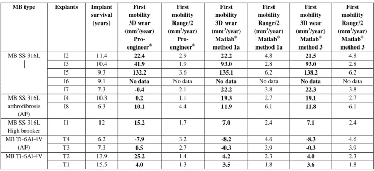
Table 3: Results of annual wear given by Pro/Engineer® and the two Matlab®’s methods for the first mobility of series of twelve explants.
Figure 7: Comparison of the results of first mobility annual wear for the three methods.
First of all the results given by methods 1a and 3 are not significantly different, they could be considered as similar. Compared to the results from Pro/Engineer®, they are significantly different in five cases I3, I7, I4, I1 and T2, approximately half of samples.
About the second mobility, convex side, the method 1a is adapted to calculate the annual wear for the second mobility, the method 3 is not handy to use in that case so it is adapted only twice to confirm the results obtained from method 1a. The results are presented in Table 4 and Figure 8.
Table 4: Results of annual wear given by Pro/Engineer® and the two Matlab®’s methods for the second mobility of a series of twelve explants.
Figure 8: Comparison of the results of second mobility annual wear for two methods and few results from method 3.
Once again the methods 1a and 3 are not significantly different. The comparison with the wear volumes from Pro/Engineer® showed a significant difference in two cases I4 and I1.
3.2 Surface roughness measurement
ANOVA, analysis of variance, enables to compare means of two or more series of samples given their distribution is normal, their variance equal and they are independent and random. These last two requirements were fulfilled since the five measures are taken by turning the cup randomly with an approximate angle of 40° and 80° for the worn and no-worn zones respectively. Besides the ANOVA test is known to be robust regarding the two other assumptions, all the more as the number of measures were equal for all series.
Comparison between optical and mechanical profilometers
The global comparison of the two techniques resulted in only one significant difference which is for the parameter Sdr and for the worn zone. This is the only case the statistical tests concluded the two profilometers gave significantly different results.
Worn/no-worn zone comparison
Other ANOVA tests are performed to know in what cases the mechanical and the optical profilometers are able to distinguish wear. We might think that if two techniques distinguished worn zones the explant would be considered worn. Otherwise we could not be surewear is significant. Obviously it is of great interest to know if a zone of an explant is worn or not. The comparison of the results from the two profilometers and the mean comparison tests can give this kind of answer. The results are presented in Table 5.
Table 5: Results of ANOVA tests (p=0.05) between the worn and no-worn zones to know in what cases the two profilometers distinguish wear.
The mechanical profilometer distinguished wear for three cups I3, I5 and I6 for most parameters. The optical profilometer distinguished wear for I5 only four times for both I3 and I5 for three parameters. The results are very similar except that the optical profilometer seemed to detect wear less often. We saw similar results for Sa, St, Sdr and Srk and they are less interesting for the two other parameters so one decided to focus on the most relevant parameters Sa and Sdr. Indeed Sa gives general information and it is the most commonly used parameter, Sdr is the most differential parameter in the related study and, unlike Sa, it enables to differentiate a peaked surface from a plane one.
Cups comparison
The last series of ANOVA tests enabled to compare the cups one by one to see if the value of each parameter is significantly different from the others. That is performed for the mechanical and the optical measurements separately. The aim is to adjust the ranking made on the means since one did not know for sure if a cup placed after another one in the ranking is significantly different or could be considered identical. There are a total of twelve rankings but one focused on Sa, Figures 9 and 10 and Tables 6 and 7.
Figure 9: Sa values for every cup and both techniques (mechanical and optical profilometer) on the no-worn zone ranked according to the mechanical technique.
The ANOVA test with the Bonferroni’s correction resulted in no significant difference between any of the thirteen cups for the optical profilometer. So it could be concluded that no ranking could be established for the optical technique which made the comparison of techniques impossible. However it is worth noticing that none cup is significantly different from the blank cup for both methods which is reassuring since they are not supposed to be worn in the no-worn zone.
The Figure 10 and the tables 6 and 7 present the results for the Sa parameter in the worn zone.
Figure 10: Sa values for every cup and both techniques on the worn zone ranked according to the mechanical technique.
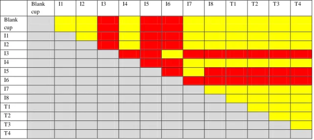
Table 6: ANOVA results (p=0.05) for the mechanical profilometer on the worn zone for the parameter Sa, yellow indicates no significant difference, red indicates a significant difference.
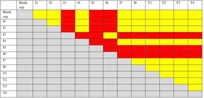
Table 7: ANOVA results (p=0.05) for the optical profilometer on the worn zone for the parameter Sa, yellow indicates no significant difference, red indicates a significant difference.
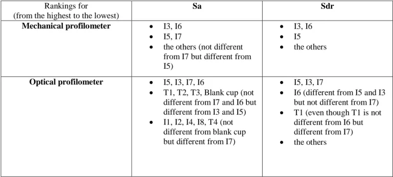
Firstly the cups ranking (from the highest Sa values to the lowest) is never exactly the same between the mechanical and the optical techniques. However the same trends are observed. Generally the highest values measured with the mechanical profilometer corresponded to the highest values measured with the optical one except for a few cases like I2. But the error is so high that it could be said as different for sure. This is the reason why statistical test, One-way ANOVA test, is used; it is of interest to know with a high confidence which cups are different from the others. Then, based on these tables from the ANOVA tests it is possible to make a new ranking. For the mechanical technique this ranking would be:
-I3, I6 // I5, I7 // the others (not different from I7 but different from I5). For the optical technique it would be:
-I5, I3, I7, I6 // T1, T2, T3, Blank cup (not different from I7 and I6 but different from I3 and I5) // I1, I2, I4, I8, T4 (not different from blank cup but different from I7).
These two rankings are quite similar.
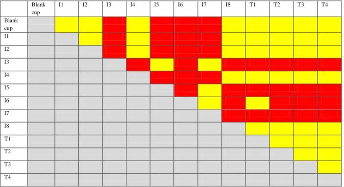
The second parameter one focused on in that study is Sdr. It is the most significant parameter when the mechanical profilometer is used. The same conclusion as for Sa could be made for the no-worn zone. For the worn zone, figure 11 presents the ranking of the Sdr average values according to the mechanical technique and the tables 8 and 9 show the ANOVA results about the cups comparison for each method.
Figure 11: Sdr values for every cup and both techniques on the worn zone ranked according to the mechanical technique.
Table 8: ANOVA results (p=0.05) for the mechanical profilometer on the worn zone for the parameter Sdr, yellow indicates no significant difference, red indicates a significant difference.
Table 9: ANOVA results (p=0.05) for the optical profilometer on the worn zone for the parameter Sdr, yellow indicates no significant difference, red indicates a significant difference.
The new ranking for the mechanical profilometer is the following: -I3, I6 // I5 // the others
The ANOVA tests also enable to adjust the ranking for the optical profilometer, it becomes:
-I5, I3, I7 // I6 (different from I5 and I3 but not different from I7) // T1 (even though T1 is not different from I6 but different from I7) // the others
Again profilometers look similar about the cups comparison. All the rankings are presented in the following table 10.
4. Discussion
4.1 Wear calculation by CMM
First of all the comparison of the relative errors showed that methods 1a and 3 are the most appropriate to calculate worn volumes since they gave the closest volumes compared to Pro/Engineer®. It appeared also that the original number of points from CMM was sufficient to get satisfying results regarding that measured zone. Besides the worn volumes from Pro/Engineer®, and methods 1a and 3 are quite similar since the largest relative errors are respectively 0.64% and 0.85%. However the average annual wear calculated with these methods gave sometimes results significantly different from the results given by Pro/Engineer®. It is thought to be due to the tolerances, the fact that one had to take them into account to calculate the theoretical volumes added an inaccuracy. Indeed when an explant is chosen it had already been manufactured so the actual diameter could be known, the error about the tolerances had already been taken into account. A difference between the theoretical volumes is noticed which resulted from three different methods used to calculate it. It raises the question of using a different method to calculate the theoretical volume and the palpated one. However it might be more consistent to use the same to calculate both. Therefore a difference in the theoretical volumes added to the even slight difference in palpated volumes can entail large difference in wear volumes since the scale is much smaller for wear volumes (the maximum order of magnitude is 1,000 mm3 compared to about 7,000 mm3 for the palpated volumes), all the more as if the two differences are not in the same direction. Therefore it is not sufficient to have the tolerances to calculate accurately the wear volume since these tolerances introduce a quite large error in the results. The ideal situation would be to know the exact volume before implantation in order to be able to calculate wear without taking into account the manufacturing tolerances but only the errors introduced by the CMM. Unfortunately it is not achievable since these measurements should be made after manufacturing and should be kept in the implant file. Blunt et al. preferred another solution. They considered the unworn zone as the reference, i.e. the implant before implantation. They reconstructed the whole unworn volume by interpolating the points measured in the unworn zone with a non-uniform rational B-splines NURB [1]. They obtained wear scar maps showing the deviations from the worn surface in good agreement with observations.
As the methods arehave been validated, the three results could be considered as valid, hence all of them had to be taken into account to give volumetric wear range. As a result it could be quite large, for instance for the first mobility of the explant named I3, the average annual wear is between 40.0 mm3/year and 95.8 mm3/year. Nevertheless the values found are in agreement with the ones from the literature, for example 21.5 ± 3.2 mm3/Mc (Mc means million of cycles and one Mc corresponds to about a year of gait) for a dual mobility prosthesis in a hip simulator [25], or 21.5 mm3/Mc for a simple mobility implant under smooth conditions in a hip simulator as well simulating normal walking [6]. Moreover Affatato et al. compared the wear performance of UHMWPE and cross-linked polyethylene (XLPE), they measured wear by a gravimetric method. Three acetabular cups of each are run in a simulator during three millions cycles and six control cups are used to correct the soak effect. They calculated a wear rate of 37 mm3/Mc for UHMWPE [26]. It is worth noting that tests with hip walking simulator do not take into account the microseparation and the movement with high angles. Other studies performed explants wear analysis. For instance Hall et al. presented wear measurements of 129 explanted Charnley prosthesis comprised of a stainless steel femoral ball and a UHMWPE socket. The diameter of the head is 22.25 mm and the thickness of the socket is 10 mm. They used a shadowgraph technique to assess wear. They found a wear rate of 55 (SE=5) mm3/year [10]. It is
similar to the values we found. Besides, Jasty et al. studied the volumetric wear for 128 acetabular components in polyethylene retrieved after autopsy or after revision. They used a fluid-displacement method found to be accurate to within 10%. They found values between 8 and 284 mm3/year [11]. Therefore the results of the present study are in agreement with the values in the literature even though the methods used could be very different. Some techniques are not used anymore and yet they gave similar results. Actually the results range found for a same technique even a same study is so broad that it is difficult to compare the techniques.
The fact that the results from method 1a and 3 are similar may mean that the approximation of a spherical segment is not too rough since method 3 did not use this approximation at all. Besides the largest asymmetrical wear is noticed for the explant I3 and the relative errors are respectively 0.18% and 0.67% for method 1a and 3. Therefore this approximation might be considered valid even in critical cases but it would require more tests on critical cases to be sure it is always valid.
Limitation remains since the mechanical stylus of the CMM could not palpate the whole surface. Wu et al. already highlighted the probe accessibility difficulty linked to its actual size [27]. A new CMM device should be available for measuring wear volume in the concave side. Small head of the CMM and a moving plateau with fixed cup should be useful for measuring the entire wear volume on the concave total face.
There is an improvement of the CMM machine since an articulating arm is installed. It enables to palpate a larger surface. However, for weak grooves in the material, the mechanical stylus filters the exact heights of each measured point as it could penetrate the surface a little. Indeed such a thin tip in diamond is likely to dig into polyethylene. Therefore the calculated wear is a minimum limit. The true wear is likely to be higher, all the more as the bottom of the insert could not be accessed by the stylus. This assessment could be confirmed by [28]. Plastic behavior of asperities could occur under stresses
4.2 Surface roughness measurement Global technique comparison
The fact that the ANOVA test performed for each zone taking the series of thirteen cups resulted in only one difference showed that the two methods, mechanical and optical profilometers, give similar results. Indeed Sdr is the parameter the most inclined to be different since it exacerbates the errors the most. Besides the worn zone is the most irregular so this difference could be due to the measurement locations instead of the profilometers themselves. Therefore, this only difference allowed concluding that they gave similar results in most cases.
Worn/no-worn zone comparison
First of all, one could conclude from the comparison of worn and no-worn zones: the I3 and I5 cups are worn for sure since both techniques had detected it. Then it appeared that both techniques could distinguish wear for the same cups, I3 and I5. However the optical profilometer failed to distinguish wear for I6 but it may be due to a digging effect of the stylus from the mechanical method. Consequently the roughness detected was likely to be a bit exaggerated and it might have considered that there was slight wear whereas the optical profilometer did not detect this error. Or, it could come from the optical profilometer that could see the holes but could not detect them if the slope of patterns was too high, upper than 40°. Therefore in that particular case the mechanical profilometer, initially
thought as less accurate due to the mechanical stylus; it should not be neglected for profilometry analyses related to wear.
The two cups for which both techniques distinguished wear had the stainless steel metal-back. It is not surprising not to detect wear for the cups with the Ti-6Al-4V metal-back since it just slightly rubbed, wear did not occur like the others. Moreover there are four cases of fibrosis (I4, I8, T3, T4) the hip mobility was highly limited which explained wear is not detected [9]. The remaining cases which are thought to wear normally and yet the profilometers did not distinguish it are I1 and I2. However I2 is suspected to have an intermediary state of fibrosis and I1 worn only slightly as observed in Table 3 compared to the other explants with a stainless steel, 316L, metal-back. Consequently the results were in agreement with the explants characteristics.
Cups comparison
The ranking and the cups comparison for Sa and Sdr parameters showed that for the no-worn zone the ranking given by both techniques could be the same since there is no significant difference between any of the values measured by the optical technique. Besides the zone called no-worn zone seemed to be indeed no-worn since the twelve results given by both techniques are not significantly different from the blank cup.
Several conclusions could be made for Sa in the worn zone. First the cups different from the blank cup are the cups for which the corresponding method is said to distinguish wear. The rankings of the cups according to their Sa values after ANOVA tests for both techniques are very similar so again both techniques could be seen as equivalent. Besides I3, I5, I6 and I7 are on the left of the blank cup in the ordered ranking, thus they must be more striated than the blank cup which would correspond to a wear domain after polishing i.e. after about 9 years of implantation. Indeed I3, I5 and I6 had a survival time equal or higher than 9 years. Note that it is different for I7 since it is not significantly different from I3, I5 and I6 but not different from the blank cup neither. Hence its roughness must be lower, so must be its survival time. The others are more polished than the blank cup, which corresponded to a wear domain between 0 and 9 years. Other authors noticed a well-polished zone on worn implants [11]. It is the case except for I2, I4, T1 and T2. However T4 had fibrosis, I2 is suspected to have it too and the metal-backs in Ti-6Al-4V follow a particular wear process. Ssk is said to be a parameter of interest for describing the wear process since we know if there are more valleys or more peaks. However the ANOVA tests highlighted the fact Ssk is not able to detect significant difference between the worn and no-worn zone or between the cups. It could be concluded that due to the too high uncertainty errors Ssk cannot allowed to draw any conclusion about the methods comparison or the wear mechanisms in this case.
The Sdr parameter is interesting for a comparison purpose since it exacerbated the differences. At first the results given by the mechanical and the optical methods seemed very different. It is possible to explain the general tendency that the mechanical results are lower than the optical ones. Indeed the stylus used in the mechanical machine is thought to squash the surface, moreover the asperities could be unseen and the developed area is smaller than reality.
As expected the results are similar to the ones from the Sa analysis. In the worn zone the cups for which the methods distinguished wear are significantly different from the blank cup so it is relevant. Again the rankings are very similar and allowed to separate the cups between the most altered (I3, I5, I6) and the cups more polished than the blank cup since the developed area is equal or lower. The optical profilometer seemed to differ from the mechanical one for I6 and I7; it described I6 as less worn and I7 as more worn. It is confirmed by the fact that the mechanical profilometer gave a higher
Ssk value for I6 (0.67 against 0.02). The Ssk value for the I7 cup on the worn zone is more similar (0.28 and 0.20) so one could not be sure about the location of I7 in the wear process.
Therefore, generally for the cups thought to have worn normally (i.e. without fibrosis and with a stainless steel metal-back) the roughness parameters seemed to indicate an abrasive process which is in agreement with literature. Indeed Jasty et al. observed some highly polished area in the worn zone separated from the less worn zone by a ridge and some multidirectional scratching. They concluded to abrasive and adhesive wear. However they did not separate wear mechanisms of explants according to the implantation time ranging from 1 to 21 years [11].
Some differences remained between both techniques but they could be explained by the fact that the mechanical method is a contact method unlike the optical one. Besides, the samples could have been deteriorated a little since the mechanical measurements. It cannot be due to the sampling that is good enough in this analysis. The optical profilometer took more points since it had a better resolution which would make it the best method. However it is limited by the slope inclination of the holes and by the fact that the UHMWPE material absorbed a little which altered the reflection. Therefore first of all it can be concluded that one method is not always better than the other but one must choose the more adapted to its issue. Secondly both techniques are proved to give similar results in this kind of explants analysis. Finally in this type of analysis the mechanical profilometer was not less accurate than the optical profilometer, it is of great interest to use the results from both and the ANOVA tests to draw conclusions about the explants wear.
Some limitations can be evoked. First the measures are not made at the exact same locations and we are not assured to avoid a very particular zone with a very different roughness affecting the results. However, performing five measures all around the cup is a mean to avoid this kind of problem. Another limitation is the fact that the surface roughness measurements are not carried out on the inner surface. Therefore we could not draw conclusion for the techniques comparison in the particular case of dual mobility but we had to be more general. Nevertheless this limitation came from the set-up not adapted to the inner measurements. Therefore further measurements will have to be performed using another set-up to complete the study.
Conclusion
Wear analysis is crucial in numbers of applications like the orthopedic implants field. Indeed wear is a major cause for implants failure, so the wear process must be studied to increase the prostheses longevity. The right instrument to use depends a lot on the applications. The purpose of this paper is to compare some methods in the particular application of Metal-on-Polymer (MoPpolymer is UHMWPE) dedicated to dual mobility explants analysis. Indeed they are likely to differ from simple mobility implants in the wear performance.
It could be concluded from the present study that CMM together with a software like Pro/Engineer® or Matlab® can be used to calculate wear. Depending on the software used, the range would be different but in agreement with the order of magnitude found in other studies. Besides if several softwares are used the range was broader but it was also closer to reality. The relevant point was ranking wear of dual mobility cups thanks to wear volumes from CMM data. CMM has already been proven to be efficient for wear analysis, our study proved that this efficiency does not depend on the post treatment since using two different techniques gave similar results. It is already said in other studies that CMM could be adapted for the explants wear analysis; the current study makes the same conclusion in the
particular case of dual mobility. It is of interest to confirm it is applicable to that particular type of implants since they are used more and more. Besides it is not deducible from the studies on simple mobility since in the case of dual mobility there are inner and outer surfaces of UHMWPE that wear. Moreover it is seen that the results are in the same range as in the literature for dual or simple mobility. Consequently with present designs the benefits of less dislocation seem not to be counterbalanced by a higher wear which is encouraging for further development of this dual mobility concept. Nevertheless the volumetric wear ranges are so broad that it is difficult to conclude to a similar wear for sure.
Moreover in addition to quantitative information, qualitative information can be obtained from profiling techniques. Basically there are contact and non-contact techniques but the most suitable method depends on the application. In the application mentioned in that paper it has been seen that the mechanical profilometer should not be neglected as it did not give less accurate results. Even though the accuracy of z-axis measurements is better for the non-contact profilometer, i.e. optical, the mechanical one allows providing better measurements especially in the worn zones. Besides it seems that the same abrasive mechanisms than for simple mobility are involved. Nevertheless further studies will have to be performed on the inner surface to be sure it is the same for both friction surfaces even if the surface area is different. It suggests that development of new design can pursue the same goals as for simple mobility. Moreover the same analysis should be investigated for testing in-vitro, firstly, and in-vivo, secondly, of new material as cross-linked and/or melted UHMWPE, for example. Methods which are presented in this work, should allow improving these new materials.
With the technological progress more and more advanced techniques have been developed, they enable to give more accurate results on a smaller scale because of a better resolution. One might suggest the Atomic Force Microscopy, AFM, investigations could be relevant for qualitative analyses. The key issue seems to be the simultaneous rotating plate that is supporting the cup. For optical and mechanical profilometers or AFM, it should be a good way of development.
These new techniques should be used in the particular application of explants analysis to see if they enable to get more information about the wear mechanisms. The final aim is to measure the wear volume of UHMWPE cup as close as possible to the actual value. Thus the study of new materials, cross-linked and/or remelting UHMWPE, for decreasing wear should be relevant for better lifetime of hip prosthesis, especially the couple Metal on Polymer, MoP.
Acknowledgments
The authors acknowledge Mr. Eric Laisne for technical help about the optical profilometry. They are grateful the Region Rhône-Alpes for supporting the stay at Penn State University, State College PA USA.
References
[1] L. Blunt, P. Bills, X. Jiang, C. Hardaker, G. Chakrabarty, The role of tribology and metrology in the latest development of bio-materials, Wear 266 (2009) 424-431.
[2] S.L. Bevill, G.R. Bevill, J.R. Penmetsa, A.J. Petrella, P.J. Rullkoetter, Finite element simulation of early creep and wear in total hip arthroplasty, J. Biomech. 38 (2005) 2365-2374.
[3] S.H. Teoh, W.H. Chan, R. Thampuran, An elasto-plastic finite element model for polyethylene wear in total hip arthroplasty, J. Biomech. 35 (2002) 323-330.
[4] J.S.S. Wu, J.P. Hung, C.S. Shu, J.H. Chen, The computer simulation of wear behavior appearing in total hip prosthesis, Comput. Meth. Prog. Bio. 70 (2003) 81-91.
[5] T.A. Maxian, T.D. Brown, D.R. Pedersen, J.J. Callaghan, A sliding-distance-coupled finite element formulation for polyethylene wear in total hip arthroplasty, J. Biomech 29 (1996) 687-692.
[6] J.G. Bowsher, J.C. Shelton, A hip simulator study of the influence of patient activity level on the wear of crosslinked polyethylene under smooth and roughened femoral conditions, Wear 250 (2001) 167–179.
[7] V.A. González-Mora, M. Hoffmann, R. Stroosnijder, F.J. Gil, Wear tests in a hip joint simulator of different CoCrMo counterfaces on UHMWPE, Mat. Sci. Eng. C 29 (2009) 153–158.
[8] S. Affatato , M. Spinelli, M. Zavalloni, C. Mazzega-Fabbro, M. Viceconti, Tribology and total hip joint replacement: Current concepts in mechanical simulation, Med. Eng. Phys. 30 (2008) 1305–1317.
[9] J. Geringer, B. Boyer, F. Farizon, Understanding the Dual mobility concept for total hip arthroplasty. Investigations on a multiscale analysis, Wear 271 (2011) 2379-2385.
[10] R.M. Hall, A. Unsworth, P. Siney, B.M. Wroblewski, Wear in retrieved Charnley acetabular sockets, Proc Instn Mech Engrs 210 (1996) 197-207.
[11] M. Jasty, D.D. Goetz, C.R. Bradgon, K.R. Lee, A.E. Hanson, J.R. Elder, W.H. Harris, Wear of polyethylene acetabular components in total hip arthroplasty, The Journal of Bone and Joint Surgery 79-A (1997) 349-358.
[12] B. Morris, L. Zou, M. Royle, D. Simpson, J.C. Shelton, Quantifying the wear of acetabular cups using coordinate metrology, Wear 271 (2011) 1086-1092.
[13] M. Tuke, A. Taylor, A. Roques, C. Maul, 3D linear and volumetric wear measurement on artificial hip joints-Validation of a new methodology. Precis. Eng. 34 (2010) 777-783.
[14] H.C. Kandpal, D.S. Mehta, J.S. Vaishya, Simple method for measurement of surface roughness using spectral interferometry, Opt. Laser. Eng. 34 (2000) 139-148.
[15] B. Dhanasekar, B. Ramamoorthy, Digital speckle interferometry for assessment of surface roughness, Opt. Laser. Eng. 46 (2008) 272-280.
[16] U.P. Kumar, B. Bhaduri, M.P. Kothiyal, N.K. Mohan, Two-wavelength micro-interferometry for 3-D surface profiling, Opt. Laser. Eng. 47 (2009) 223-229.
[17] K.J. Stout, L. Blunt, Nanometers to micrometers: three-dimensional surface measurement in bio-engineering, Surf. Coat. Tech. 71 (1995) 69-81.
[18] C.Y. Poon, B. Bhushan, Comparison of surface roughness measurements by stylus profiler, AFM and non-contact optical profiler, Wear 190 (1995) 76-88.
[19] J-P. Yun, S-P. Chang, T-B. Xie, L-L. Zhang, G-Y. Hu, A novel contact and non-contact hybrid profilometer, Precis. Eng. 33 (2009) 202-208.
[20] A. Taguchi, T. Miyoshi, Y. Takaya, S. Takahashi, Optical 3D profilometer for in-process measurement of microsurface based on phase retrieval technique, Precis. Eng. 28 (2004) 152-163.
[21] V.G. Badami, S.T. Smith, J. Raja, R.J. Hocken, A portable three-dimensional stylus profile measuring instrument, Precis. Eng. 18 (1996) 147-156.
[22] D. Najjar, M. Bigerelle, H. Migaud, A. Iost, About the relevance of roughness parameters used for characterizing worn femoral heads, Tribology International 39 (2006) 1527–1537.
[23] A.M. Brown, A new software for carrying out one-way ANOVA post hoc tests, Comput. Meth. Prog. Bio. 79 (2005) 89-95.
[24] F. Curtin, P. Schulz, Techniques and Methods Multiple Correlations and Bonferroni’s Correction, Biol. Psychiat. 44 (1998) 775–777.
[25] V. Saikko, M. Shen, Wear comparison between a dual mobility total hip prosthesis and a typical modular design using a hip joint simulator, Wear 268 (2010) 617–621.
[26] S. Affatato, G. Bersaglia, M. Rocchi, P. Taddei, C. Fagnano, A. Toni, Wear behavior of cross-linked polyethylene assessed in vitro under severe conditions, Biomaterials 26 (2005) 3259-3267.
[27] Y. Wu, S. Liu, G. Zhang, Improvement of coordinate measuring machine probing accessibility. Precis. Eng. 28 (2004) 89-94.
List of figures
Figure 1: Schematic of a dual mobility implant; * is related to the first mobility between head and cup; ** corresponds to the second mobility between cup and metal back. Two motions are possible.
Figure 2: Algorithm for the palpated volumes and annual wear calculations. The methods are selected and validating for the inner part of the insert.
Figure 3: Spherical segment (colored), its height is H. Two spherical caps of height h1 and h2 complete the sphere of radius R. Its center is approximated to be (0,0,Cz).
Figure 4: Spherical segment (colored) of height h=h1+h2.
Figure 5: The volume is calculated by addition of each cylinder (circle area multiplied by the height, example in orange where we use the above half height plus the below half height).
Figure 6: Comparison of first mobility palpated volumes for Pro/Engineer® and the two methods selected. Figure 7: Comparison of the results of first mobility annual wear for the three methods.
Figure 8: Comparison of the results of second mobility annual wear for two methods and few results from method 5.
Figure 9: Sa values for every cup and both techniques on the no-worn zone ranked according to the mechanical technique.
Figure 10: Sa values for every cup and both techniques on the worn zone ranked according to the mechanical technique.
Figure 11: Sdr values for every cup and both techniques on the worn zone ranked according to the mechanical technique.
List of tables
Table 1: Table of the measurements performed on each implant.
Table 2: Relative errors of the worn volume (in %) for the five methods compared to Pro/Engineer®’s results; bold characters are related to the smallest errors; I6 is not palpated by CMM.
Table 3: Results of annual wear given by Pro/Engineer® and the two Matlab®’s methods for the first mobility of series of twelve explants.
Table 4: Results of annual wear given by Pro/Engineer® and the two Matlab®’s methods for the second mobility of a series of twelve explants.
Table 5: Results of ANOVA tests (p=0.05) between the worn and no-worn zones to know in what cases the two profilometers distinguish wear.
Table 6: ANOVA results (p=0.05) for the mechanical profilometer on the worn zone for the parameter Sa, yellow indicates no significant difference, red indicates a significant difference.
Table 7: ANOVA results (p=0.05) for the optical profilometer on the worn zone for the parameter Sa, yellow indicates no significant difference, red indicates a significant difference.
Table 8: ANOVA results (p=0.05) for the mechanical profilometer on the worn zone for the parameter Sdr, yellow indicates no significant difference, red indicates a significant difference.
Table 9: ANOVA results (p=0.05) for the optical profilometer on the worn zone for the parameter Sdr, yellow indicates no significant difference, red indicates a significant difference.
120407 JET 1207.
Reviewing process.
Comments from authors related to questions of reviewers. Italic is dedicated to show Reviewer #1: Introduction:
Generally please re-write this to add clarity for the reader - for example, extend the detail relating to each methodology discussed and provide some critical evaluation of the references cited (e.g. the Blunt study)
‘Unfortunately it is not achievable since these measurements should be made after manufacturing and should be kept in the implant file. Blunt et al. preferred another solution. They considered the unworn zone as the reference, i.e the implant before implantation. They reconstructed the whole unworn volume by interpolating the points measured in the unworn zone with non-uniform rational B-splines NURB [1]. They obtained wear scar maps showing the deviations from the worn surface in good agreement with observations.’ It is the part of the text for discussion about the Blunt’s Study.
Please check reference 1 as this does not correspond with the statements regarding aseptic loosening and wear.
Page 2: “The most common cause of premature failure of implanted joints is aseptic loosening, accounting for 75% of revision operations. Aseptic loosening can be attributed to macrophage (immune system) response to particulate debris generated by wear of the components, and bone resorption due to stress shielding after prosthesis implantation”
Please add further detail regarding the rationale of the study and the expected outcomes.
These sentences were added at the end of the paragraph: “One might expect finding wear volume with better accuracy. Moreover, the investigations about 3D profilometry should allow improving the best method dedicated to understand the wear mechanism.”
Please add further information/definition of the dual mobility hip concept.
Figure and the paragraph ‘The dual mobility concept was invented in the 1970s by Professor Gilles Bousquet. The dual mobility implant consists in a small metallic head moving within an acetabular cup in Ultra High Molecular Weight Polyethylene (UHMWPE). This latter is moving within a metal-back (fig.1). It is of interest to measure the wear performance of this kind of implants to compare them to simple mobility implants. In a previous study [9] the wear of the acetabular cup was assessed quantitatively and qualitatively using a CMM and profilometers. In this study we compared wear measurement methods from the CMM data and we compared the mechanical and optical profilometers.’ were added in order to better understand the dual mobility concept.
Methods:
The materials section is not easy to read, nor to refer back to whilst reading the rest of the document, could the authors create a table to aid the clarity of this section?
The table 1 was added for clarifying this section. *Revision Notes - list of changes and response to referees
2.1 Wear Calculation
Could the authors consider re-defining the methods as 1 (a-c) and then 2, 3 as there is no significant difference in the first 3 methods, and it would assist the reader if the second method defined is method 2.
The table 2 has been changed according to your advice. 2.2 Surface roughness measurement
Please consider adding an image to assist the reader with the identification of the measurement locations
A schematic of the zones location can be found in the reference [9]. If not sufficient, authors might add the figure related to [9].
Please summarise paragraph 2 and add to the introduction
The paragraph 2 is adapted in introduction. According to your advice, the paragraph was shortened. Please add a figure to support the definition of the surface parameters paragraph 4 –
Authors suggest that definitions of roughness parameters are presented in some references [22] and [9]. The authors hope this paragraph is useful for better defining the roughness parameters: ‘In the already mentioned related study the most relevant parameters for differentiating the worn zones from the no-worn zones were identified as Sa, Sq, Ssk, St, Srk, Sdr [9]. [9] and [22] help understand the meaning of these parameters. Sa, Sq and Ssk are amplitude parameters, St is a spatial parameter, Srk is an Abbott-Firestone parameter and Sdr is a hybrid parameter. Ssk is the skewness that is the degree of asymmetry of a surface height distribution about a mean plane. It is interesting for wear measurements since a positive Ssk indicates the preponderance of peaks and a negative Ssk the preponderance of valleys. A peak is defined as a point above its eight nearest neighbors and a valley is defined as a point below its eight nearest neighbors. St is the sum of the largest peaks height and the largest valleys depth, therefore it is more sensitive to the surface than Sa or Sq. Srk (or Sk) is the depth of the working part of the surface that is the main flat part. Sdr is the developed interfacial area ratio, it is a percentage defining the additional surface area due to the texture compared to the plane surface of the same size. Even though the difference in Sa is small, the difference in Sdr can be large so this parameter enables to differentiate surfaces with similar mean roughness but a difference in texture as Sdr increases with the number of peaks and valleys.’
please could the authors clarify how they will be comparing the profiling methods when it appears the measurements have not been conducted in the same location?
For sure we could not measure at the same location, exactly, for mechanical and optical profilometry. We should imagine a kind of Laser disposal for finding the same position in the space on each cup. For CMM this kind of device is available according to our knowledge but it was not possible to use this kind of apparatus on different profilometers. It is the reason why we concentrated our attention on specific zones related to wear. We can conclude that measurements were performed by zone.
Results
Please could the authors provide the rationale for comparing the present methods with the ProEngineer method by relative error - has the ProEngineer method been shown to be correct, or is this comparing an error with a non-absolute value?
Pro Engineer® is considered as the ‘gold standard’, i.e. the reference. From results issued from this
method, all others are compared as following:
Could the authors add some context to both the wear and surface measurements, by comparing with typically reported clinical data where possible?
It is of interest to measure wear. The Pro-e® in designing implants is nowadays to reduce wear [1,
ref Blunt].
It is of interest to measure the surface roughness and topology to be able to understand the wear mechanisms, the main ones seem to be abrasive and adhesive wear [11, ref Jasty; 26, ref Affatato] Cups comparison: Could the authors re-write the paragraph commencing 'At first sight' as it is presently confusing - perhaps a table could assist the ranking.
Table 10 was added in order to assist the ranking Discussion:
Please add further comparison with other studies in terms of wear and surface measurement techniques, in addition to the wear data presented.
We added comparisons with studies that used CMM but it is too complicated to do the same for the surface roughness measurements. Indeed it depends too much on the machine, the protocol… therefore it is not consistent to compare the roughness parameters values. Nevertheless we can compare our conclusions with theirs regarding the methods comparison.
In addition, could the authors comment on the measurement techniques employed to assess wear in these studies compared with the present study.
The authors added the following part about wear measurements, comparison between this study and other ones: ‘As the methods were validating, the three results could be considered as valid, hence all of them had to be taken into account to give volumetric wear range. As a result it could be quite large, for instance for the first mobility of the explant named I3, the average annual wear was between 40.0 mm3/year and 95.8 mm3/year. Nevertheless the values found were in agreement with the ones
from the literature, for example 21.5 ± 3.2 mm3/Mc (Mc means million of cycles and one Mc
corresponds to about a year of gait) for a dual mobility prosthesis in a hip simulator [25], or 21.5 mm3/Mc for a simple mobility implant under smooth conditions in a hip simulator as well simulating
normal walking [6]. Moreover Affatato et al. compared the wear performance of UHMWPE and cross-linked polyethylene (XLPE), they measured wear by a gravimetric method. Three acetabular cups of
each were run in a simulator during three millions cycles and six control cups were used to correct the soak effect. They calculated a wear rate of 37 mm3/Mc for UHMWPE [26]. It is worth noting that tests
with hip walking simulator do not take into account the microseparation and the movement with high angles. Other studies performed explants wear analysis. For instance Hall et al. presented wear measurements of 129 explanted Charnley prosthesis comprised of a stainless steel femoral ball and a UHMWPE socket. The diameter of the head was 22.25 mm and the thickness of the socket was 10 mm. They used a shadowgraph technique to assess wear. They found a wear rate of 55 (SE=5) mm3/year
[10]. It is similar to the values we found. Besides, Jasty et al. studied the volumetric wear for 128 acetabular components in polyethylene retrieved after autopsy or after revision. They used a fluid-displacement method found to be accurate to within 10%. They found values between 8 and 284 mm3/year [11].
Therefore the results of the present study are in agreement with the values in the literature even though the methods used could be very different. Some techniques are not used anymore and yet they gave similar results. Actually the results range found for a same technique even a same study is so broad that it is difficult to compare the techniques.’
Could the authors also comment on potential refinements or developments that might improve the accuracy of the assessed wear of the explant?
Measurements of wear volume should involve potential refinements, as you mentioned. The authors discussed about this point in two rearranged paragraphs.
‘Global technique comparison
The fact that the ANOVA test performed for each zone taking the series of thirteen cups resulted in only one difference showed that the two methods, mechanical and optical profilometers, give similar results. Indeed Sdr is the parameter the most inclined to be different since it exacerbates the errors the most. Besides the worn zone is the most irregular so this difference could be due to the locations of the measure instead of the profilometers themselves. Therefore, this only difference allowed concluding that they gave similar results in most cases.
Worn/no-worn zone comparison
First of all, one could conclude from the comparison of worn and no-worn zones: the I3 and I5 cups were worn for sure since both techniques had detected it. Then it appeared that both techniques could distinguish wear for the same cups, I3 and I5. However the optical profilometer failed to distinguish wear for I6 but it may be thought to be due to a digging effect of the stylus from the mechanical method. Consequently the roughness detected is likely to be a bit exaggerated and it might consider that there is slight wear whereas the optical profilometer does not detect this error. Or, it could come from the optical profilometer that can see the holes but cannot detect them if the slope of patterns is too high, upper than 40°. Therefore in that particular case the mechanical profilometer, initially thought as less accurate due to the mechanical stylus; it should not be neglected for profilometry analyses related to wear.’