Assessing strategies for reducing carbon emissions associated with wood products transportation

(1)

ASSESSING STRATEGIES FOR REDUCING CARBON

EMISSIONS ASSOCIATED WITH WOOD PRODUCTS

TRANSPORTATION

Mé moire

Mingqian Zhang

Maîtrise en génie mé canique

Maître è s sciences (M.Sc.)

Qué bec, Canada

(2)

ASSESSING STRATEGIES FOR REDUCING CARBON

EMISSIONS ASSOCIATED WITH WOOD PRODUCTS

TRANSPORTATION

Mé moire

Mingqian Zhang

Sous la direction de :

(3)

RÉSUMÉ

Suite à la ratification par le Canada de traités de réduction des émissions de gaz à effets de serre (GES), différents paliers de gouvernement ont mis en œuvre des politiques visant la réduction des émissions industrielles et liées au transport. Depuis 2013, le Québec, conjointement avec la Californie et l’Ontario, ont mis en place un marché du carbone pour encourager les entreprises à réduire leurs émissions. L’industrie forestière, s’appuyant sur le transport de marchandises, pourrait bénéficier de ce régime en termes de prise de décision sur la planification du transport.

Cette étude vise à analyser le potentiel des stratégies de réduction des émissions de carbone et à proposer des suggestions appropriées sur la prise de décision en matière de la planification du transport. Quatre stratégies sont principalement envisagées : la réduction de la vitesse, la conduite écologique, le transport intermodal et les modes de chargement. Combinant les stratégies, des modèles d'optimisation dont l'objectif est de minimiser des coûts sont développés sous les contraintes des émissions. Ces modèles impliquent la planification de la distribution de la gestion de la chaîne d'approvisionnement et des problèmes de tournées de véhicules. Microsoft Excel, OpenSolver, Gurobi et LocalSolver sont principalement utilisés pour la modélisation et l’optimisation. Un front de Pareto est par la suite utilisé pour illustrer la relation entre le coût de transport et les émissions de carbone.

Pour démontrer les méthodologies, une étude de cas est présentée en utilisant des données réelles. Il est constaté que l'éco-conduite présente un potentiel de réduction des émissions intéressant dans une gamme réaliste d'augmentation des prix. Le choix des stratégies varie selon les préférences du décideur et la difficulté de mise en œuvre des stratégies.

(4)

ABSTRACT

With the ratification of greenhouse gas (GHG) reduction agreements by Canada, various levels of government implemented policies to reduce transport-related and other industrial emissions. Since 2013, Québec, together with California and Ontario, has established a carbon market to encourage firms to reduce their emissions. The forest industry could benefit from this scheme in terms of improving efficiency and lessening the environmental impact of wood product transport.

This study aims to assess the potential of carbon emission reduction strategies and to provide recommendations on improving the logistics of transporting wood-based materials. There are four main strategies considered in this paper; namely low-speed driving, eco-driving, intermodal transportation, and optimizing loading pattern. By combining these strategies, optimization models are developed with the objective of cost minimization under the constraints of emissions. These models involve the distribution planning of supply chain management and routing problems. Microsoft Excel, OpenSolver, Gurobi, and LocalSolver are mainly used for modeling and optimization. Pareto Front is also used to illustrate the relationship between transportation cost and carbon emission.

To demonstrate the methodologies, a case study is exhibited using real world data. It is found that eco-driving has considerable potential in reducing emissions under a feasible range of price increases. The selection of strategies is based on the decision makers’ preferences and the difficulty of strategy implementation.

(5)

LIST OF TABLES

Table 2.1 Recent studies on fuel economy and carbon emission reduction resulting from speed decrease and eco-driving ... 19 Table 4.1 The dimensions of lumbers in foot and maximum number of packs loaded in a 53-foot truck trailer ... 44 Table 4.2 Transportation cost and emission of routes on speed of 105 km/h on road

... 45 Table 4.3 Transportation cost and emission of routes on speed of 95 km/h on road 46 Table 4.4 Transportation cost and emission of routes with eco-driving ... 47 Table 4.5 Transportation cost and emission of routes on intermodal transportation48 Table 4.6 Percentage of trips with each transportation mean for set #1 ... 53 Table 4.7 Percentage of trips with each transportation mean for set #2 ... 54 Table 4.8 Percentage of trips with each transportation mean for set #3 ... 54

(8)

LIST OF FIGURES

Figure 1.1 Canada’s GHG Emissions by Economic Sector in 2013 (Environment

Canada, 2015) ... 2

Figure 1.2 Quebec’s GHG Emissions by Economic Sector in 2013 (MDDELCC, 2016) ... 3

Figure 1.3 The Québec cap and trade scheme for emission allowance (Government of Quebec, 2016) ... 5

Figure 3.1 Methodology with the broad types of data coming into the steps ... 26

Figure 3.2 Rear-end view of a 53-ft truck trailer ... 30

Figure 3.3 Display of a Carbon RoadMap layer (Vallerant, 2013) ... 32

Figure 3.4 Example of Combination of lumbers in groups ... 39

Figure 4.1 Pareto Front of transportation cost and emission of model #1 ... 53

Figure 4.2 Pareto Front of heuristic model #3 using multi-product loading patterns with full shipment of data set #1 ... 56

Figure 4.3 Pareto Front of simplified model #4 with multi-product loading patterns with full shipment ... 57

Figure 4.4 Comparison of Pareto Front of model #1 and simplified model #4 using multi-product loading patterns ... 58

Figure 4.5 Comparison of simplified and heuristic models using multi-product loading patterns ... 59

(9)

ACKNOWLEDGEMENTS

I would like to express my appreciation to the people who have invested their time in my research and have accompanied me throughout this academic journey.

First and foremost, I would like to thank my supervisor, Dr. Marc-André Carle, whose enlightening instruction, impressive kindness and patience helped guide me through my thesis and my graduate student life.

Secondly, I wish to express my special thanks to Professor Jonathan Gaudreault. He provided me with a great opportunity to experience studying and conducting research at Laval University and to work with great people at the research consortium FORAC. I am truly indebted to FORAC for its unwavering confidence in my abilities and for the resources made available to me, which have made my studies in Canada financially possible.

In addition, I shall extend my gratitude to Dr. Achille-Benjamin Laurent, whose direction was critical in the completion of this research paper. I would also like to extend my deep appreciation to my friend, Alexander Lee, who spent precious time proofreading the thesis.

Furthermore, I am also very grateful for my friends in Canada for making this time unforgettable: Ahsan Alam, Xiao Tong Guo, Vanessa Simard, Blandine Carel, Sabreena Anowar, Duo Zhang, Xiaowei Wang, Yutai Liu, Kanyi Huang and Ruixi Liu.

Finally, I would like to thank my boyfriend Junshi Xu, my parents, who love me and have supported me unconditionally during my time at Laval University.

(10)

CHAPTER 1. INTRODUCTION

1.1 Context and background

1.1.1 Greenhouse gas (GHG) and carbon emissions

The greenhouse effect is caused by greenhouse gas. Gases like carbon dioxide can absorb thermal energy and prevent solar radiation from reflecting off the atmosphere, resulting in increased temperatures on the earth’s surface and lower atmosphere. Without this effect, the average temperature of earth’s surface would decrease below the freezing point of water. On the contrary, if the greenhouse effect were to be more pronounced, global temperature would continue to increase year by year. Ultimately, it would worsen the ecological environment and change global climate by causing climate anomalies, sea-level rise, and an increase of arid land (Intergovernmental Panel on Climate Change, 2013).

The greenhouse gases (GHGs) are mainly composed of water vapour (H2O), carbon

dioxide (CO2), methane (CH4), and ozone (O3), which contribute to roughly 36-70%,

9-26%, 4-9% and 3-7% of the greenhouse effect respectively on the earth’s surface (Ram, 2014). In addition, there are some other secondary GHGs such as nitrous oxide (NOx),

sulfur hexafluoride (SF6), hydrofluorocarbons (HFCs), perfluorocarbons (PFC), and

chlorofluorocarbons (CFCs) that also play a role in influencing the greenhouse effect, Although the global-warming potential (an indicator to represent the capacity of gases to contribute to the greenhouse effect) of these aforementioned gases is higher than that of carbon dioxide, their concentrations in atmosphere are not considerable. While H2O is one

key component of GHGs, its unique properties allow it to convert to different states in atmospheric circulation, and thus the content of water vapour in the atmosphere keeps balanced stability. However, CO2, along with concentrations of other GHGs, are heavily

(11)

is therefore imperative to reduce the quantity of carbon emissions for mitigating greenhouse effect by adapting human activities (Solomon, Qin, & Manning, 2007). For this reason, the concentration of CO2 is set as the standard unit for measurement of the overall

greenhouse effect, which is called carbon dioxide equivalent (CO2 eq.).

From 1990 to 2011, the global GHG emissions increased by 42%. In the year of 2012, Canada’s gross emissions, having risen by 25.5% compared to those in 1990, accounted for 1.6% of the global GHG emissions (U.S. EPA, 2006). According to statistics in 2013, when analyzing emissions by economic sector, it was found that transportation was the second largest contributor to Canada’s GHG emissions, which accounted for 23% of total emissions. The other key segments were oil and gas (25%), electricity (12%), buildings (12%), emissions-intensive and trade-exposed industries (11%), agriculture (10%), as well as waste and others (7%) (See Figure 1.1) (Environment Canada, 2015).

Figure 1.1 Canada’s GHG Emissions by Economic Sector in 2013 (Environment Canada, 2015)

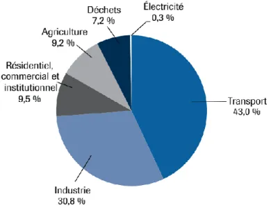
Correspondingly, transportation made up 43% of total GHG emissions in the province of Quebec in 2013. Moreover, industry (30.8%), residential, commercial and institutional

(12)

emissions (9.5%), agriculture (9.2%), waste (7.2%) and electricity (0.3%) were also key contributors to GHG emissions (see Figure 1.2) (MDDELCC, 2016).

Figure 1.2 Quebec’s GHG Emissions by Economic Sector in 2013 (MDDELCC, 2016)

1.1.2 GHG Protocol and carbon trading

In 1997, the Kyoto Protocol was signed as the supplementary provision of United Nations Framework Convention on Climate Change (UNFCCC) in Kyoto, Japan. This protocol aimed to stabilize the concentration of GHGs in the atmosphere at an appropriate level in order to prevent dramatic climate change. Having signed the Kyoto Protocol, Canada pledged to cut down on its GHG emissions to 94% of 1990 levels (461 Megatons) between 2008 and 2012. Although Canada declared to withdraw from this protocol in 2011, it indicated a significant attempt for Canada to reduce GHG emissions. Furthermore, in Quebec, the government promised that it would achieve the goal of curtailing GHG emissions by 20% by and 30% by 2030 compared to the level of GHG emissions in 1990 (MDDELCC, 2015).

(13)

A new type of market for trading allowances of carbon emissions has recently been put in place by governments known to many as the carbon market. The cap and trade allowance scheme is an environmental policy instrument aimed to conserve energy and reduce emissions. It aims to encourage firms or individuals to reduce business carbon emissions and to invest and innovate in clean technologies for achieving environmental protection goals (Groenenberg & Blok, 2002). When a cap and trade system is implemented, the government sets a binding limit (called a “cap”) each year and distributes an emission allowance for each market participant in the system, meaning that a certain amount of free carbon credits is allocated to participants. Moreover, emission allowances could be collected from offset credits of unregulated emissions and early reductions credits. In order to reduce overall emissions, the allocated allowance of each participant is reduced each year by a certain percentage (Grubb, 2012).

In 2012, Quebec’s cap and trade system was published, which was formally linked with California’s system on 1st_{January 2014, becoming the largest carbon market in North}

America. In the cap and trade system, market participants that emit 25,000 tons or more of CO2 eq. per year are regulated. For the first compliance period (2013-2014), only the

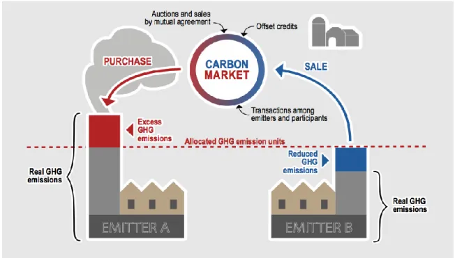
industrial and electricity sectors are subject to the system. Fossil fuel distributors are also included in the system during the second and third compliance period (2015-2017 and 2018-2020). As of today, 132 entities or qualified bidders have joined in this cap and trade system. Overall, GHG emissions by sector include stationary combustion, transport, industrial processed solvent and other product use, and agriculture and waste (International Carbon Action Partnership, 2017a). At the end of each compliance period, all covered emitters should have enough allowance to cover their reported or audited GHG emissions. As shown in Figure 1.3, if the quantity of carbon emitted by the participant exceeds its allowance, the emitter ought to pay for the exceeded emissions by auctioning from governments or by purchasing from other companies. On the contrary, it can sell its surplus

(14)

carbon emissions credits to other participants in the carbon market (Gouvernement du Quebec, 2014). Therefore, covered emitters should make trade-offs between the cost of purchasing their extra carbon emissions and the cost of improvement of production and transportation processes for reducing their carbon emissions (Flachsland, Marschinski, & Edenhofer, 2009).

Figure 1.3 The Québec cap and trade scheme for emission allowance (Government of Quebec, 2016)

To establish this system, carbon emissions should be calculated based on a unified standard such as GHG protocol. GHG Protocol was established in 1998 and published in 2001 by World Resources Institutes and World Business Council for Sustainable Development, aiming to provide standards of counting and reporting GHG emissions for business so that firms or countries could use this protocol to set a target of GHG reduction (Schmitz et al., 2004).

(15)

When calculating GHG emissions, the firm must also take into consideration its operational boundaries. It should choose scopes for identifying emissions with its operations in order to avoid double counting. These scopes are classified by direct GHG emissions (Scope 1), electricity indirect emissions (Scope 2) and other indirect GHG emissions (Scope 3). Direct GHG emissions refer to GHG emitted by operations owned or controlled directly by the firm, such as fuel combustion on transportation (i.e. company-controlled vehicle fleet) and production procedures on equipment. Scope 2 refers to indirect emissions from purchased or consumed electricity. These two scopes must be counted and reported by companies. Scope 3 refers to other indirect GHG emissions such as extraction and transportation of raw materials. This scope enables GHG emissions generated upstream and downstream to be accounted for. Furthermore, it provides firms with standards to assess and choose supply chain partners, as firms could reasonably distribute limited sources by a better understanding of indirect emissions to effectively achieve emission reduction targets and maximize returns on investment.

For participants of cap and trade system in Quebec and California, Scope 1 and Scope 2 are used to calculate carbon emissions in order to summarize the quantity of carbon trade. A firm should first identify sources of GHG emissions within Scope 1, such as stationary combustion, mobile combustion, process emissions and fugitive emissions. For the forest industries, process emissions primarily indicate emissions from the production of pulp and paper. If they own or operate vehicle fleets, emissions from mobile combustion should be reported and paid. Then the firm should identify sources of indirect emissions from the consumption of purchased electricity, heat, and steam, which are covered by Scope 2. Finally, these emissions are estimated by selected calculation approaches indicated in GHG Protocol and summed up and reported to cooperate level (Schmitz et al., 2004). In terms of fuel consumption in cap and trade system, fuel suppliers who sell more than 200 litres of fuel per year are not given allowances free of charge and need to purchase them at

(16)

auction or from the carbon market, while fuel consumers such as carriers can calculate their GHG emissions covered by Scope 2 and offset or trade them in the market (Government of Quebec, 2016).

1.1.3 Impacts of freight transportation

As mentioned earlier in the paper, the transportation sector, as the second largest contributor behind the oil and gas sector, comprised 23% of total GHG emissions in Canada in 2013 (Environment Canada, 2015). This category encompasses both passenger and freight transportation. Freight transportation can be further subdivided into five sectors: on-road heavy trucking, off-road, marine, rail, and intermodal. In 2008, the first four segments contributed 70%, 11%, 11% and 8% respectively to GHG emissions within the freight transportation sector in Canada (Sustainable Development Technology Canada, 2009). The report also indicates that GHG emissions increased by 12.6% in industrial freight transportation from 2002 to 2006, with heavy trucks being a principal cause of the increase (ibid.). Furthermore, statistical records for 2006 showed that industrial transportation accounted for 12.1% of total end-use energy in Canada (ibid.). For Canada to meet its commitments toward emissions reductions, a thorough investigation on reducing GHG emissions in the context of freight transportation remains of utmost significance.

1.1.4 Forest industry

In 2013, 12% of Canada's manufacturing GDP was attributed to the forest products industry (Eds, 2015). There is great potential in reducing the future carbon footprint of the forest industry due to the rapidly expanding market of wood products, especially for construction materials. Compared to cement or concrete, wooden materials are more environmental friendly, as the production and operation of wood products emit less carbon (Börjesson &

(17)

Gustavsson, 2000; Gustavsson, Pingoud, & Sathre, 2006). Moreover, the wooden buildings can be recyclable and less energy intensive (Gao, Ariyama, Ojima, & Meier, 2001).

In addition, the regional shipping of forest products is reliant on heavy-duty truck and rail transport. Research has shown that the forest products industry is one of the largest freight rail users along with coal, mining and chemical industries, and the forest industry alone accounts for about 20% of total annual revenue generated by the Canadian National Railway Company (CN) and 5% revenue for the Canadian Pacific Railway (CP) (Forest Products Association of CANADA, 2010). The forest products industry is proven to be one of the most significant industrial users of the surface transportation system in Canada (ibid.).

Given primary resource industries’ dependence on freight transportation, coupled with the new policy of carbon trade in Québec, it is crucial for companies within the Québec forest products industry to consider the adverse ecological impacts associated with freight transportation, which should be calculated and classified under the aforementioned Scope 2 or Scope 3 (provided that the company does not use its owned vehicle fleets but rather subcontracts to other carriers) based on the GHG Protocol. The forest industry sector’s largest emitters, pulp and paper mills, are covered in the cap and trade system as they own their sawmills, and thus there is an opportunity to conduct enterprise-wide reduction (Gouvernement du Quebec, 2014).

1.2 Research purpose

Environmental problems are emerging with the development of global industries and market economy, as well as concerns regarding current regulations of carbon emissions in mitigating the greenhouse effect. The carbon-trading scheme implemented in Quebec from

(18)

2013 onwards has proven to be one of the most effective ways in the province’s mitigation efforts. The forest products industry contributes a substantial quantity of carbon emission, both directly and indirectly through its use of freight transportation services. As a result, we must examine the potential for GHG emissions reductions through improving freight transportation services, which in turn would benefit firms according to the carbon trading allowance scheme.

This study concentrates on the analysis of potential strategies for carbon emissions reduction by conducting transportation cost optimization under the implementation of the cap and trade system for GHG emissions in the value chain of the Quebec forest products industry. It aims at proposing feasible methods of reducing carbon emissions associated with supply chain and transportation activities and allowing firms to benefit from Quebec’s cap and trade scheme to the fullest extent. There are various reduction methods in regards to freight transportation activities having been proposed and elaborated in the existing literature. Four appropriate and potential methods to decrease carbon emissions in the logistics chain of the forest products industry, specifically pertaining to transportation, are discussed in this study. A case study is explored in this study by implementing optimization models for supply routes around Lac Saint-Jean in Quebec. Potential emission reductions are then calculated and compared. The methods are evaluated based on the cost of implementation and the potential carbon reduction.

1.3 Structure of thesis content

This document consists of five parts. Chapter 1 is designed to provide some context to the application of the cap and trade scheme in forest industry companies regarding transportation planning. Chapter 2 provides a summary of recent studies in green freight transportation and related methods of emissions reduction in supply chains, and will also

(19)

delve into various tools and models to assess GHG emissions. Chapter 3 will follow by investigating approaches for developing optimization models to provide a transportation plan taking into account the new carbon trade rules. Chapter 4 presents a case study to explain and discuss potential emission reduction strategies. Finally, the thesis concludes with Chapter 5, summarizing major findings as well as limitations that would benefit from future research.

(20)

CHAPTER 2. LITERATURE REVIEW

With unprecedented growth in international trade and commerce in recent years, demand in freight transport has been noticeably increasing. However, the environmental ramifications of choosing freight cannot be neglected. A number of studies have taken green freight transportation into consideration, which aims to minimize emissions to the greatest extent while making transportation cost-effective. It is worth noting that as the predominant component of GHG, CO2 is in direct proportion to fuel consumption, thus

fuel-saving issues are pertinent when creating solutions to reduce emissions (ICF Consulting, 2006). The following literature review is focused solely on three aspects: the transportation planning framework within the logistics chain; methods or strategies for fuel efficiency improvement in addition to carbon emission reduction; and models and approaches to estimating the emission reduction.

2.1 Transportation and Distribution Planning

Transportation plays a crucial role in the logistics chain, facilitating the movement of materials from the supplier to the client (Tseng, Yue, & Taylor, 2005). The distribution and transportation process identifies how products are distributed and transported from supplier to customer (Lee & Kim, 2002). Transportation planning can be organized hierarchically through strategic, tactical and operational levels. Strategic planning represents the tip of the hierarchy and refers to a firm’s long-term planning of transportation policy. This level primarily determines the introduction of policies or the establishment of infrastructure such as determining optimal facility location. Tactical decision-making concerns the allocation of existing resources and design of service networks, including transportation route choice, work allocation among terminals, and operation of service. Operational planning is often considered to be the most dynamic level. This level refers to details such as quantities of

(21)

deliverable goods to be shipped, the use of service, the logistics of dispatching vehicle fleets among other items. This hierarchical system ensures effective inter-communication between different decision-making levels, where operational planning policies are conducted by terms dictated by the higher levels. Moreover, the lower level can use specific models addressing specific problems and provide system performance feedback and recommendations to the higher level to assist in future decision-making processes, thereby increasing the flexibility of the decision-making system as a whole (Crainic & Laporte, 1997). Furthermore, the transportation planning model combines a variety of factors under certain constraints in order to achieve specific objectives, particularly that of cost minimization. In this study, distribution and transportation problems are tied to issues related to the tactical level.

The Vehicle Routing Problem (VRP) is one of the more prevalent transportation planning problems, which refers to issues in finding optimal routes with the shortest traveled distance in order to ship products to customers under side constraints. Bektaş and Laporte (2011) proposed an extension of the VRP called Pollution Routing Problem (PRP). The purpose of the PRP does not only focus on economic costs, but also on environmental effects and social impacts (Bektaş & Laporte, 2011). There is a trend that green freight transportation has been considered in the process of decision making. Economic costs and environmental effects are considered as bi-objective in this study when the transportation planning model is built.

2.2 Strategies for carbon emission reduction on logistics chain

Green freight transportation has become a trending issue across the globe in recent years. In Europe, a project named SuperGreen has been completed successfully in 2013. The United States has also begun implementing innovative ideas and moving towards a

(22)

progressively eco-friendly direction, with the United States Environmental Protection Agency (EPA) having collaborated with the freight sector to run a program called SmartWay Transport. In addition, the Global Green Freight Action Plan, which is under the Climate and Clean Air Coalition (CCAC) to reduce short-lived climate pollutants, has been developed by the United Nations Environment Program and various countries including Canada. A presentation at the 2013 conference of the Transportation Association of Canada (TAC) introduced and compared five green trucking programs across different regions of Canada, namely The Green Fleets (Enviro-truck) Program, Trucks of Tomorrow, The GrEEEn Trucking Program, Ontario Green Commercial Vehicle Program (OGCVP), and FleetWiser (Greening the Fleet Rebate Program). These projects and programs not only focus on the improvement of freight transportation efficiency but also take into account the reduction of adverse effects on the environment and on society as a whole from the perspective of governments and commercial institutions.

The European Chemical Industry Council and the Association Européenne du Transport de Produits Chimiques (Cefic-ETCA) introduced several potential areas of improvement aimed at reducing carbon emissions (Cefic-ECTA, 2011) related to freight transportation. The study identified six points: modal shift, supply chain management, increase of vehicle utilization by decreasing the proportion of empty running, increase of vehicle utilization by increasing the payloads, the fuel efficiency of vehicles, and carbon intensity of fuel. There are subdivided methods under these listed aspects, such as avoiding unnecessary routes, shifting road transportation to greener rail transportation, and improving vehicle design and operation could all be of concern.

A previous study proposes more than 50 potential best practices for decreasing GHG emissions in freight transportation, among which some can also be examined in this paper (H. Frey & Kuo, 2007). These practices are organized in terms of transportation modes

(23)

involving truck, rail, air, water, and pipeline transport. In addition, they indicate that methods in mitigating GHG emissions can be further sub-classified through reducing energy use and altering fuels. Out of total 59 identified practices, the costs of 13 cost-effective methods were assessed by collecting information from published reports and studies (ibid.). Five of these thirteen methods are related to road transportation, which is directly relevant to the supply chain of the forest products industry. These practices include off-board truck stop electrification, auxiliary power units, direct-fired heaters, hybrid trucks, and B2 biodiesel for trucks. This paper also points out that it is possible to achieve emission reductions on the order of 85% if the long-haul truck is replaced with a combination of rail and truck transport (ibid.).

Many studies focused on factors influencing carbon emissions from freight transportation have proposed key recommendations to decrease emissions. The Canadian government published a number of resources outlining fuel-efficient driving techniques to achieve a greener and more sustainable future in 2011 (Urban Environmental Programs, 2011). The Physics of MPG presented a series of methods of fuel economy on diesel engines, which also noted that shape character of the truck trailer can influence fuel consumption (The Physics of MPG, 2007).

One significant publication has summarized a number of factors that influence fuel consumption and presents a variety of fuel consumption models (E. Demir, Bektaş, & Laporte, 2014). These factors are mainly divided into five essential categories, including vehicle, environment, traffic, driver, and operations. Some of the factors related to mechanical improvement, environmental conditions and infrastructure include the features of engines, the shape of vehicles, altitude, and pavement types. The influences of driving speed and driver behaviour on GHG emissions in the freight transportation are also examined in this thesis.

(24)

In conclusion, there are various approaches that can be examined in this study. Four highlighted strategies are chosen: intermodal transportation, low-speed driving, eco-driving, and optimizing loading patterns. They will be discussed separately in the following sections.

2.2.1 Intermodal transportation

Intermodal freight transportation, which is defined as providing transportation services using more than one mode of transportation, has developed into a significant component to support trade globalization in transportation systems. It has been used to improve the efficiency and lower costs of distribution but it can also be used to reduce the emissions associated with transportation (Emrah Demir, Bektas, & Laporte, 2011).

In general, the levels of emissions from rail and water transportation are reported in the literature to be lower than those from road transport (Husdal, Jensen, Sorkina, & Port, 2012). The capacity of rail and water transportation is also more sizeable than that of road transport. The Iowa Department of Transportation (IowaDot), responsible for the construction, maintenance, and organization of the highway system in the U.S. state of Iowa, compares the cargo capacity of different transportation modes: the capacity of one barge is equal to that of 16 rail cars or that of 70 large truck trailers (Iowa Department of Transportation, 2016). However, road transport has an advantage in terms of time efficiency, especially in situations where long-distance shipping is required. Because of the specific requirements of rail or water infrastructure which are not accessible or connected with mills and customers in most instances, the rigidness in terms of flexibility provided by rail and sea transportation is inferior to that of road transport (K. M. R. Hoen, Tan, Fransoo, & Houtum, 2013).

(25)

By combining the benefits of each mode, intermodal transportation enables the system to be more efficient, cost-effective and sustainable (Mulligan & Lombardo, 2006). With the increasing exchanges of commodities, railways and short sea shipping (SSS) have been prioritized in the European Union’s transportation policy as supplements to road transport, which presents numerous negative externalities in environmental terms and through traffic-related issues such as congestion, accidents, and noise. (López-Navarro, 2014). In Canada, the use of intermodal traffic rose by 32.6% from 2005 to 2014 (Railway Association of Canada, 2015).

Moreover, there is also research conducted to quantify environmental aspects and incorporate them into the decision-making processes in studies on intermodal transportation. A study assessing impacts of intermodal transportation on the environment concluded that it was substantially more environmentally friendly to use intermodal freight transportation rather than unimodal road transport when only considering energy use and emissions (Kreutzberger, Macharis, Vereecken, & Woxenius, 2003). In another study, environmental impact was considered in network optimization models of intermodal freight (Winebrake et al., 2008). Other research proposed to introduce environmental costs into transportation planning models with the objective of minimizing time and emissions (Bauer, Bektaş, & Crainic, 2010).

As mentioned in the introduction, the shipping of forest products primarily depends on heavy duty truck and rail in the region of North America. In this thesis, intermodal transportation refers to a combination of road and rail transportation.

(26)

2.2.2 Low-speed driving

Apart from intermodal transportation, there are some other potential methods of reducing fuel consumption. The most significant method is vehicle speed reduction as it is highly correlated to inertia, rolling resistance and air resistance, which influence the instantaneous engine load (Emrah Demir, Bektaş, & Laporte, 2014). A number of academic research have emphasized the potential of improving fuel economy by reducing driving speeds. A previous study in Belgium on the external costs of interurban freight traffic was based on a relationship between emissions and average speed of trucks for calculating the emissions of light duty and heavy trucks (Beuthe, 2002). In addition, a study in Netherlands focusing on modeling full cost of an intermodal and road freight transport network took advantage of the same average speed of each vehicle making a round trip of approximately the same length (Janic, 2007). Furthermore, another study regarding the emissions resulted from vehicle routing and scheduling also highlighted the significance of the speed over distance traveled (E. Demir et al., 2014).

The relationship between emission rates and travel speed has been demonstrated in the literature to be non-linear (Figliozzi, 2011). More specifically, fuel consumption and the emission rate of CO2 per mile traveled decreased with the increase of vehicle speed

operating up to optimal speed, before starting to increase again (Hong, 2014). In real driving conditions, there was a rapid non-linear growth in emissions and consumption as travel speeds dropped below 48 km/h (Barth & Boriboonsomsin, 2008). CO2 emission per

mile doubled when the speed decreased from 48 km/h to 20 km/h or when the speed decreased from 20 km/ to 8 km/h (Figliozzi, 2011). Over 48 km/h, the change of CO2

emission was not evident until speeds reached 80km/h, with CO2 emission per mile

(27)

2.2.3 Eco-driving

In the context of real-world transportation networks, congestion significantly influences CO2 emissions and fuel efficiency. This is due to the fact that congestion is associated with

idling and low-speed driving, which result in a rise in emissions. As fuel consumption is a function of not only speed but also acceleration rates, frequent changes in speed will increase emission rates (H. C. Frey, Rouphail, & Zhai, 2008).

A number of studies have investigated strategies on improving the efficiency of fuel consumptions. Some researchers have carried out experiments and concluded that if companies would be able to achieve approximately a 15% reduction in emissions if they developed better routing operations to avoid stop-and-go traffic situations (Baumgartner, Léonardi, & Krusch, 2008; Suzuki, 2011).

In addition to limiting acceleration practice and route choice, improving driving practice is one of the most cost-effective and eco-driving methods for reducing fuel consumption. It can have a positive impact on fuel economy regardless of technological issues associated with the vehicle (Ang-Olson & Schroeer, 2002). An effective driving program should take into account monitoring driver performance after the practice based on the data from electronic engine monitors to analyze detailed performance over time. Meanwhile, it is worth considering providing drivers with incentives to reduce fuel consumption, such as salary or vacation bonuses. If appropriately designed and implemented, driver training is found to be a very effective and efficient tool in improving driving behaviour. A number of studies have shown that driver training programs could improve fuel economy and result in fuel savings ranging from 5% to 20% (Liimatainen, 2008; Porter et al., 2013; Rakotonirainy, Haworth, Saint-Pierre, & Delhomme, 2011).

(28)

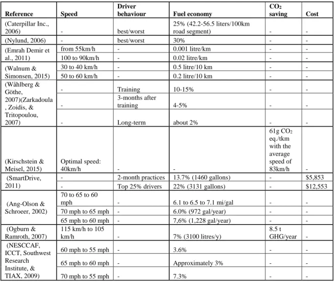
Table 2.1 summarizes the findings from previous studies on fuel economy and carbon emission reduction resulting from vehicle speed decreases and eco-driving. It provides the corresponding information and achievement in terms of fuel economy, CO2 emission

reduction, and cost-saving.

Table 2.1 Recent studies on fuel economy and carbon emission reduction resulting from speed decrease and eco-driving

Reference Speed

Driver

behaviour Fuel economy

CO2 saving Cost (Caterpillar Inc., 2006) - best/worst 25% (42.2-56.5 liters/100km road segment) - - (Nylund, 2006) - best/worst 30% - - (Emrah Demir et al., 2011) from 55km/h - 0.001 litre/km - - 100 to 90km/h - 0.02 litre/km - - (Walnum & Simonsen, 2015) 30 to 40 km/h - 0.5 litre/10 km - - 50 to 60 km/h - 0.2 litre/10 km - - (Wåhlberg & Göthe, 2007)(Zarkadoula , Zoidis, & Tritopoulou, 2007) - Training 10-15% - - - 3-months after training 4-5% - - - Long-term about 2% - - (Kirschstein & Meisel, 2015) Optimal speed: 40km/h - - 61g CO2 eq./tkm with the average speed of 83km/h - (SmartDrive, 2011)

- 2-month practices 13.7% (1460 gallons) - $5,853

- Top 25% drivers 22% (3131 gallons) - $12,553

(Ang-Olson & Schroeer, 2002) 70 to 65 to 60 mph - 6.1 to 6.5 to 7.1 mi/gal - - 70 mph to 65 mph - 6.0% (972 gal/year) - - 65 mph to 60 mph - 7,6% (1,228 gal/year) - - (Ogburn & Ramroth, 2007) 115 km/h to 105 km/h - 7% (3100 litres/y) 8.5 t GHG/year - (NESCCAF, ICCT, Southwest Research Institute, & TIAX, 2009) 60 mph to 55 mph - 3.6% - - 65 mph to 60 mph - Approximately 3% - - 70 mph to 55 mph - 7.3% - -

A previous study indicated that 40 km/h was regarded as a steady and optimal speed for keeping the heavy truck running in the lowest fuel consumption. Moreover, it also suggested that the vehicle emitted 61 g CO2 eq. /t km with an average speed of 83 km/h.

(29)

Another study illustrates that a medium freight vehicle could increase 0.001 litres of fuel per km/h from 55 km/h under the condition of null load, acceleration and road gradient. From 90 to 100 km/h, this increase peaked up to 0.02 litre per km/h (Emrah Demir et al., 2011). In addition, various other research determined that a reduction of speed from 115 km/h to 105 km/h could bring 7% saving of fuel consumption - equal to 3100 litres of fuel or 8.5 tons of GHG emissions saving per year (Ogburn & Ramroth, 2007). It also mentions that 460 million litres of fuel consumption could be saved and 1.2 million metric tons of GHG emissions reduced per year once half of Canada’s Class-8 fleet reduced their running speed to adhere to the above recommendation. Furthermore, it illustrates that fuel savings of 7.6% could be achieved if the vehicle speed is reduced from 65 mph to 60 mph (approximately from 105 km/h to 95 km/h). It is also reported that the difference in fuel consumption between the best and the worst driver regarding eco-driving ranged from 25% to 30% (Caterpillar Inc., 2006). SmartDrive Fuel Efficiency Study demonstrates that a two-month training program could reduce fuel consumption by 13.7%, and the top 25% of 695 tested heavy-duty vehicle drivers could save as much as 22% in fuel. These statistics translate to $12,553 saved if drivers were to conduct the test with 115,538 km in average annual driving distance recorded for 2011 (SmartDrive, 2011).

2.2.4 Optimizing loading pattern

There is an increasing recognition that organizations must address the issue of sustainability in their operations. Considering the comprehensive nature of the supply chain process, ranging from initial processing of raw materials to delivery to the customers, a focus on effective green supply chain management (GSCM) is a step towards maximizing energy efficiency and resource allocation (Ghatari, Hamid, Hosseini, & Shekari, 2012). GSCM is a concept derived from the traditional supply chain, which includes a firm’s internal and external actions throughout the supply chain (Fortes, 2009).

(30)

One of the key elements in the success of GSCM is the process of making optimal transportation plans (Saridogan, 2012). A previous study focused on assessing the role of logistics and transportation in GSCM reveals that technological integration with primary suppliers and with major customers was positively linked to environmental monitoring and environmental collaboration (Saridogan, 2012). Another recent study investigating the effect of reducing energy consumption in green supply chain indicates that suitable assignment of the existing transportation fleet with specified capacity could cause a reduction in energy consumption by optimizing transportation in a green supply chain (Aziziankohan, 2017).

Truckload (TL) transportation is also common in practice and supply chain agents should consider TL transportation costs and emissions in controlling their inventory and transpiration operations (Emrah Demir, Bektaş, & Laporte, 2012). There are many studies which account for basic truck characteristics such as truck capacity and truck emissions in the context of environmentally sensitive logistics operations which also focus on vehicle routing problems (Bektaş & Laporte, 2011; Jabali, Van Woensel, & De Kok, 2012; Suzuki, 2011). For instance, a study in the U.S. has included an explicit transportation model with inventory control decisions to capture per truck costs and per truck capacities. It proposed a heuristic search method to consider emission characteristics of various trucks that could be used for inbound transpiration (Konur, 2014). Another study implemented a tabu search algorithm for considering a combination of capacitated vehicle routing and three-dimensional loading (Gendreau, Iori, Laporte, & Martello, 2006).

(31)

2.3 Appropriate models to evaluate reduction methods

In the view of life cycle assessment, the processes of freight transportation can be classified into four different cycles: manufacture, maintenance, operation and disposal at the end of life (Mötzl, 2009). In this paper, GHG emissions from freight transportation primarily refer to those from the operation of freight train or truck. Almost all GHG emissions from freight transportation are caused by fuel combustion (McKinnon & Piecyk, 2010). Furthermore, carbon emission is directly proportional to fuel consumption and thus can be accurately estimated using fuel consumption figures (Kirby, Hutton, McQuaid, Raeside, & Zhang, 2000). There are two common ways to convert fuel consumption to GHG emissions - energy-based approach and activity-based approach (Cefic-ECTA, 2011).

A previous study investigated a number of fuel consumption models on road transportation, which can be used to estimate carbon emissions (Demir et al., 2014). These models can be divided into two main parts: macroscopic models and microscopic models. Microscopic models focus on the instantaneous fuel consumption and emission rates, whereas macroscopic models use average aggregate parameters to estimate network-wide emission rates. In this study, the macroscopic model is considered.

Several types of macroscopic models have been investigated in the literature. For instance, models such as Network for transport and environment (NTM) and Ecological transport information tool (ECOTRANSIT) provide friendly web engines with route distance and truckload to roughly estimate carbon emissions (K. Hoen & Tan, 2010). Other models such as COPERT (computer program to calculate emissions from road transportation) and IVE (international vehicle emissions model) provide a mechanism to get exact estimations of carbon emissions, though more detailed information such as truck engine types and fuel

(32)

types are required (ISSRC, 2008; Kouridis, Gkatzoflias, Kioutsioukis, & Ntziachristos, 2009).

Rail is treated as one of the most significant ways to ship forest products since sawmills are usually built in remote regions in proximity to forests, and where transportation infrastructure development is scarce. The capacity of a rail freight car is four or five times more than that of the freight truck. Moreover, it requires less manual labour than the truck. The crucial aspect of rail freight transportation is that it emits fewer emissions than the truck if shipping the same quantity of goods. CN company, which provides supply chain services with its rail facilities, puts forward a tool based on GHG Protocol to calculate and compare the quantities of carbon emissions from truck, rail and marine vessel. This model estimates emissions based on traveled distance at a macroscopic level. The fundamental emissions factors are distance, total freight weight, and freight weight per railcar/truck. Estimated results of total emissions could then be displayed online.

As previously mentioned, GHG Protocol offers a standard to classify and gather carbon emissions. It also provides tools to calculate GHG emissions (National Council for Air and Stream Improvement Inc. (NCASI), 2005) according to various sectors or sources, including GHG emissions models from transport or mobile sources. The level of required data is modest; for road freight transportation, information related vehicle type, traveled distance and total weight of freight would be required. These methods of estimation are similar to the method of calculating the emissions of intermodal transportation in this study, which are introduced in the next chapter.

The above research has contributed in important ways to the understanding of strategies for reducing carbon emissions in freight transportation. However, they have not considered

(33)

transportation planning in response to the concerns of reducing carbon emissions associated with freight transportation on logistic chains. This study investigates four strategies of emission reduction including intermodal transportation, low-speed driving, eco-driving, and optimizing loading pattern together for a transportation plan taking into account the new carbon trade rules at a tactical level.

(34)

CHAPTER 3. METHODOLOGY

This chapter covers the methodology of the decision-making on transportation planning in consideration of the rules of the carbon trade scheme. As mentioned in the previous chapter, the hierarchical decision-making focused in this study is at the tactical level. The objective of tactical planning is to achieve the goals of the strategic plan using the allocated resources derived from the strategical level. At this level, distribution and transportation problems typically come about due to route choice, transportation mode choice, use of terminals, delivery schedule generation, use of supply facilities, and space allocation among other factors. An integrated model involving all of these requirements listed is established. Additionally, the emission level is an essential factor concerned in this study, and thus the carbon budget is added in the transportation planning.

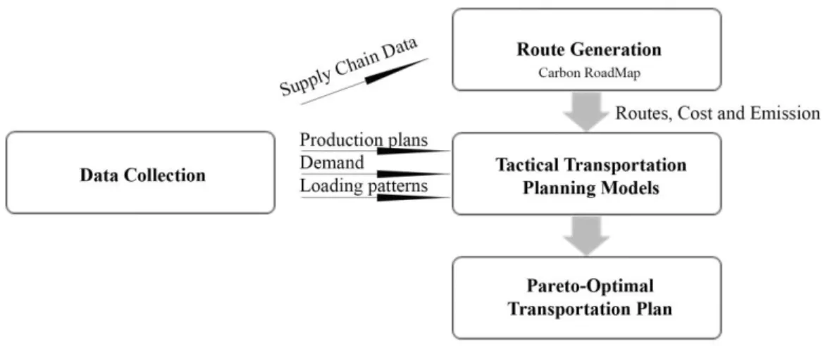
In Section 3.1, the research problem is elaborated. Section 3.2 is dedicated to the collection of required data. The next section emphasizes on Carbon RoadMap, by which appropriate delivery routes were generated. The tactical transportation planning models are then discussed in Section 3.4. Section 3.5 presents the mathematical programming solvers which were applied to solve the optimization models in this study. In the last section, Pareto Front is introduced to assess the trade-off solutions between cost and emission, with approaches to drawing Pareto Front also demonstrated. Figure 3.1 illustrates the methodology with the broad types of data coming into the steps.

(35)

Figure 3.1 Methodology with the broad types of data coming into the steps

3.1 Research problem

This study focuses on a firm producing wood products in mills, which then supplies the products to its customers. The purpose is to minimize the total cost in consideration of the carbon emission reduction. It is assumed that the demand from customers is consistent with the historical demand, and mills are able to produce wood products to meet the demand. The firm needs a transportation plan to ship wood products from mills using the appropriate transportation means to satisfy the demand (in the form of a set of customer orders, consisting of a certain quantity of different products) during one planning horizon, which typically covers several weeks.

The transportation means involved in this study are considered as methods to reduce carbon emissions, which consists of normal road freight transport, low-speed driving, eco-driving, intermodal transportation (rail and road), and multi-product loading pattern strategies for all above methods. The route choices for road and intermodal are also determined.

(36)

Moreover, space allocation for storage is also regulated so that the stock cannot exceed the demand in the following period in order to control the inventory cost.

3.2 Data collection

Firstly, customer demand is generated according to a based off of the real-world wood products market. Since demand is a function of accepted orders by the firm, it is assumed that the mills have an appropriate ability of production to satisfy the demand. In this case, the orders from customers exceeding the mills’ capacity to meet the demand would have been rejected.

Aside from the generation of demand and production plans, the data collection can be regarded as two-part corresponding to the strategies: cost and emission. As mentioned in the literature review, only cost and emissions from the operation process aspect of rail or truck are taken into consideration in this study. In addition, since fixed components such as the purchasing of trucks and office supplies are applied in all strategies involved in this study, they are not considered here as they can be offset. Moreover, GHG protocol provides the calculation tools and methods to develop comprehensive and reliable inventories of GHG emissions, not only by sectors like pulp and paper, but also for the transportation and mobile emissions in specific industries, given the quantity of fuel used, fuel combustion efficiency and the fleet size. This research followed the GHG protocol recommendations and methods to calculate emissions.

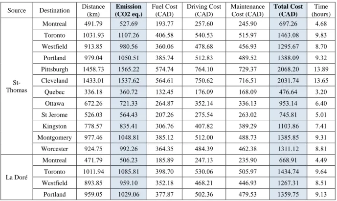
Excluding the rail portion of intermodal freight transport, the normal road freight shipping, the road component of intermodal transportation, and other transportation means take the distance, unit costs, and emissions into consideration in the model. In addition, cost consists of three additional parts: fuel cost, driving cost and maintenance cost – all of which are

(37)

proportional to traveled distance (W. Ford Torrey & Murray, 2015). The fuel cost and driving cost are also dependent on average driving speed. The driving cost involves elements such as driver wages, the use of trailers, and consumption of tires. In addition, driving cost is determined by drivers’ overall skill. The abovementioned values are for the most part collected from previous academic studies, technical reports, government announcements, and research organizations. They are specified according to the strategies in the following subsections. In the next section, Carbon RoadMap is introduced as it generates traveled distances and freight routes for each transportation mean.

3.2.1 Intermodal transportation and logistics

The intermodal routes and the terminals for transferring wood products between rail and road are generated from Carbon RoadMap. In general, the railroad offers a variety of equipment to meet different transportation requirements for all kinds of forest products. However, in order to simplify the problem, it is assumed that products are packed in a 53-foot container or beam car, which can be directly disassembled and attached to the tractor or the locomotive. Therefore, it is not necessary to repack the products during the transfer. In this study, the price and emission between rail terminals are obtained from price documents provided by railroads and price calculator on the CN website based on detailed information including origin, destination, carrier, and commodity (Canadian National Railway Company, 2010, 2017). In addition, the carrier in Canada is CN railroad, while the carrier in the United States is selected based on the region or the available service.

3.2.2 Low-speed driving

The previous literature review section summarizes recent research and reports on environmental and economic benefits from slower vehicle speeds and eco-driving. Some of the data is adopted in this study. It is worth mentioning that the data in European studies

(38)

is reported in L per 100 km for fuel consumption and km per hour for vehicle speed, while in the American studies, fuel consumption is calculated in gallons per mile and vehicle speeds in miles per hour (mph), and consequently a unit conversion is applied in the following calculation. It also needs to be mentioned that the driving speed limit is set while taking into account safety considerations. The freight vehicle is regulated to run under 105 km/h in Quebec and Ontario in Canada, and thus a speed reduction of 7.6% from 105 km/h to 95 km/h can be considered in this study.

3.2.3 Eco-driving

Driver behaviour is one of the greatest potential factors influencing fuel efficiency and carbon emissions (E. Demir et al., 2014). It affects nearly all the factors related to the operation, including the maintaining of vehicle speed, idling times, and gear selection. According to a study evaluating truck eco-driving, fuel consumption and emissions data from SmartDrive (2011) are applied in this study since it includes a reliable sample size based on the use of individualized coaching in conjunction with an in-vehicle real-time feedback system rather than simulation (Boriboonsomsin, 2015). In this study, it is assumed that eco-driving can save 13.7% of fuel consumption or reduce approximately 13.7% of carbon emissions.

3.2.4 Multi-product loading patterns

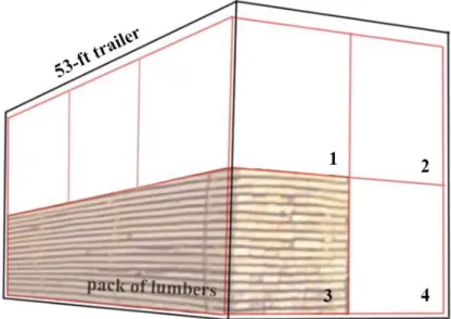
A 53-foot trailer, which is a popular choice of vehicle for freight transportation in North America, is applied in this study. Although the most common unit of measure for wood products in North America is board-foot (fbm), it is important to note that lumbers are typically assembled in packs for delivery, and customer orders always consist of a quantity equivalent to an (integer) number of packs of each product. Hence, the number of packs that can be put on a railcar depends on the length of products. It is assumed that a car trailer

(39)

can only contain four packs of wood products (two on the top and two on the bottom) in the view from one end, regardless of the product length, as shown in Figure 3.2.

Figure 3.2 Rear-end view of a 53-ft truck trailer

3.3 Route generation using Carbon RoadMap

The traveled distance of shipped wood products is directly related to transportation cost. When environmental effects or carbon emissions are considered in distribution planning, both transportation costs and delays will be influenced. Generally, costs and delays increase with the reduction of carbon emissions, as transportation means with lower emissions generally have a lower speed. It is therefore necessary for decision makers to take three criteria (cost, delay, and emission) into account so that the shipping deadlines outlined in the demands of customers are met, while transport costs and environmental impacts are reduced to the greatest extent possible.

Carbon RoadMap, a web-based decision support system, aims to find a trade-off route to transport wood products from a single source to a set of one or more destinations based on the multi-criteria decision (transportation cost, carbon emission and delivery time)

(40)

(Vallerant, 2013). This tool is mainly developed for the shipment of wood products in the North American transportation network. It uses an optimization algorithm based on the Dikjstra algorithm, which finds a set of non-dominated routes. The results are presented through an interface. Three transportation modes are considered in this system: road, rail, and ship. Routes using any combination of these transportation modes can be obtained.

Aside from the visualized routes on an actual map, the values of cost, time and emissions are presented by Carbon RoadMap for each generated route. Its manual introduces the calculation of these three criteria for a route segment, which can be expressed by one general equation (Vallerant, 2013):

c = 𝑓_𝑥+ 𝑓_𝑣 ∗ 𝑑 (3-1)

where c signifies the value of criteria, d represents the traveled distance, and fixed factor and variable factor are denoted as fx and fv respectively.

The fixed factor represents the cost, delay or emission generated during transition from one transportation mode to another if it is applied. Moreover, the variable factor is the unit value of criteria, which can be adjusted as needed. Likewise, the generation of routes requires coordinates of origin and destination or they can be directly selected on the interface. Figure 3.3 is an example displaying a Carbon RoadMap layer. The routes are visually shown in colours representing the transportation mode, and the corresponding value of the criteria is also given.

(41)

Figure 3.3 Display of a Carbon RoadMap layer (Vallerant, 2013)

Although it is impossible to guarantee that the network is complete in the Carbon RoadMap system, especially for the routes between transitions of intermodal (as waystations and intermodal facilities as additional transportation arcs are constantly added to the North American transportation network) the missing segments of routes were updated and created in this study based on data from Google Earth and using information regarding terminal positions provided by CN.

In the equation (3-1), the key variable is the distance traveled from origin to destination. For different transportation methods, corresponding fixed and variable factors are applied. In order to simplify the calculation of cost and emissions, Carbon RoadMap is used in this study to generate routes and acquire corresponding distances. It simply needs to set all variable factors as one and set fixed factors as zero in the database to examine the generated results. Two appropriate routes between an origin to a destination respectively for road and

(42)

intermodal transportation are then chosen. Finally, the values of cost and emissions are calculated for different strategies using equation (3-1) based on the corresponding distances of these routes.

Road freight transportation is the principal way of delivering wood products, while rail and ship may be used as optimizing means to reduce environmental impacts (Winebrake, Green, Comer, Corbett, & Froman, 2012). These three transportation modes are considered when Carbon RoadMap conducts the set of non-dominated routes. Generally, the ship, albeit the least efficient in terms of time, is the most economic and the eco-friendliest mode compared with other modes on the basis of ton per km. It is thus unrealistic to make use of a ship to deliver wood products if forest companies need to ship customers’ demand within a timeframe of two weeks. When hundreds of routes are generated in Carbon RoadMap, the shortest route is chosen for both road transportation and intermodal transportation. The rail acts as the main part of the route for the intermodal transportation.

3.4 Tactical Transportation Planning Models

In this section, tactical transportation planning models are introduced. Firstly, a model considers a scenario where only one product type is being transported on a trip. This model integrates the following transportation means: normal road freight transport, low-speed driving, eco-driving and intermodal transportation. The model is then modified to apply various sizes of wood products on one route trip, in order to assess the optimizing loading pattern strategy. The abovementioned transportation means are also designed in the new models, which consider a trailer containing various types of products. Two approaches are presented to solve this problem, namely a heuristic model and a simplified model.

(43)

3.4.1 General description

The optimization model of the transportation plan is described as following. A set of mills is defined as I, and J as a set of customers. Each mill i∈I produces a set of products that is defined as P. The product p∈P is planned to be shipped by mean m∈M where M = {0, 1, 2, 3}. 0∈M signifies delivering at a speed of 105km/h by road, and 1∈M denotes delivery via intermodal transportation (intermodal transportation generally combines road and rail in this research), 2 and 3 represent speed reduction (driving at speed of 95km/h) and eco-driving on the road route. The planning horizon is denoted by T.

Each customer i has a non-negative demand dpit of product p in period t∈T, and the

production quantity of product p in mill i in period t is denoted by bpjt. The units for these

two parameters are in packs since the wood products are generally sold in packs. Furthermore, cijmt is the transport cost of mean m from mill i to customer j in $ per full

truckload (FTL). As the total cost and emissions of optimization results are calculated based on the routes of each transportation mean, FTL is applied as the shipment unit in this study instead of one pack. In this case, the numbers of variables can be reduced so that the calculation is simplified, while allocation of products to trailers is not considered. As the unit is FTL, it needs to denote the number of packs of product p in a full shipment of route m as vpm. Finally, eijm represents emissions (in kilograms) associated to full shipment of

mean m and 𝐶_𝑡 stands for the upper bound of emission constraints.

Decision variables are then defined as follows: Xpijmt signifies the quantity of product p in

packs shipped from mill i to customer j by transportation mean m in period t; Lpijmt is a

non-negative integer variable denoting the number of routes of mean m used between mill i to customer j to ship product p in period t; Ipit and Ipjt respectively represent the

(44)

that the unit cost of inventory of each product is $1 per piece, so Ipit and Ipjt could directly

represent the inventory cost. I0 is denoted as the initial inventory.

3.4.2 Model #1 using single-product loading pattern The cost minimization objective of model #1 is given by

𝑀𝑖𝑛𝑖𝑚𝑖𝑧𝑒 ∑ ∑ ∑ ∑ ∑ 𝑐𝑝 𝑖 𝑗 𝑚 𝑡 ijmt𝐿𝑝𝑖𝑗𝑚𝑡+ ∑ ∑ ∑ 𝐼𝑝 𝑖 𝑡 𝑝𝑖𝑡+ ∑ ∑ ∑ 𝐼𝑝 𝑗 𝑡 𝑝𝑗𝑡 (3-2)

This objective calculates the total cost, which consists of transportation cost and total inventory cost.

The constraints of the optimization model are shown as follows:

𝐼𝑝𝑗(𝑡−1)− 𝑑𝑝𝑗𝑡+ ∑ ∑ 𝑋𝑖 𝑚 pijmt− 𝐼𝑝𝑗𝑡= 0 ∀𝑝, 𝑗, 𝑡 (3-3)

𝐼𝑝𝑗𝑡 ≤ 𝑑𝑝𝑗(𝑡+1) ∀𝑝, 𝑗, 𝑡 (3-4)

𝐼_{𝑝𝑖(𝑡−1)}+ 𝑏_𝑝𝑖𝑡− ∑ ∑ 𝑋_𝑗 _𝑚 _pijmt− 𝐼_𝑝𝑖𝑡 = 0 ∀𝑝, 𝑖, 𝑡 (3-5) 𝑋𝑝𝑖𝑗𝑚𝑡 ≤ 𝑣𝑝𝑚𝐿𝑝𝑖𝑗𝑚𝑡 ∀𝑝, 𝑖, 𝑗, 𝑚, 𝑡 (3-6)

∑ ∑ ∑ ∑ ∑ 𝑒𝑝 𝑖 𝑗 𝑚 𝑡 𝑖𝑗𝑚𝐿𝑝𝑖𝑗𝑚𝑡 ≤ 𝐶𝑡 (3-7)

Constraints (3-3) and (3-5) state that the input flow must be equal to the output flow respectively at customers and at mills. It is then assumed that the customers would not stock more wood products than the demand in the following week would allow since it would be less economical in the view of inventory planning. Constraints (3-4) define this maximum inventory at customers. Constraints (3-6) ensure that a sufficient amount of FTLs is planned in order to ship all the products for each origin- destination pair. Constraints (3-7) enforce the emissions restriction.