Agricultural spray measurement by high-speed shadow imagery

Agricultural spray measurement by high-speed shadow imagery

By N DE COCK, M MASSINON and F LEBEAU

University of Liège (ULg), Gembloux Agro-Bio Tech (GxABT)

Corresponding Author Email: nicolas.decock@student.ulg.ac.be

Summary

Spray characteristics determine treatment performance and environmental contamination. Shadowgraphy associated with high-speed imaging presents an attractive option for measuring drop velocity and size simultaneously. This study presents an overview of the contrast problems occurring when using backlighted images and proposes appropriate solutions for reliable and quality measurements. Drop diameter measurement is based on the area inside the sub-pixel contour assuming a circular shape. Drop velocity is determined by tracking a drop on two successive images taking into account the drop size, speed limits and the general flow direction. Then, the drop size distribution is corrected taking in account the sampling rate of each drop. Finally, a comparison between PDA and shadowgraphy measurements realized simultaneously on the same spray location is presented.

Key words: Agricultural spray, drop size distribution, shadowgraphy, image

analysis.

Introduction

The size and the velocity of the drops constituting agricultural sprays directly affect the treatment application efficiency. Therefore, consequent efforts have been done to classify nozzles with respect to the drop size distribution of their sprays. Most of the non-intrusive techniques used for spray characterisation are optic based, i.e., Phase Doppler Anemometry (PDA), laser diffraction spectrometry (LDS), Particle/Drop Image Analysis (PDIA). PDA measures particle size and velocity from light scattered by a particle moving through the measurement volume, created by the interferences of crossing laser beams. PDA measurement requires liquid optical properties (refractive index) and is limited to quasi spherical particle (Hirleman & Bachalo, 1990). LDS measures diffraction pattern formed by the particles inside the probe volume. Drop size distribution is found by using the complete Mie theory or the Fraunhofer approximation of the Mie theory on the recorded diffraction pattern (ISO 13320:2009). This method provides spatial measurement of particle size distribution without information on particle velocities. PDA measurement and diffraction methods require coherent light source from laser and dedicated electronics and optics, which induce a high cost. PDIA, usually performed in backlighted arrangement, is often referred as shadowgraphy. Particles significantly bigger than light wavelength located in probe volume, defined by the camera field of view and depth of field, intercept the light and cast their shadows on the camera sensor. Particle size and centroid coordinates are determined by digital analysis of its shadow. Velocity measurement requires a tracking algorithm that identifies the same particle on two successive frames. This set up provides spatial and temporal measurement of particles. This arrangement offers relatively low influence of particle shape and liquid optical properties on

particle size and velocity measurement (Lecuona et al., 2000) and requires no delicate optic alignment.

The rapid development of imaging equipment and image processing capabilities during the last decade makes shadowgraphy an ever easier and cheaper alternative to scatter or diffraction based measurement methods for low density spray. A number of manufacturers propose off-the shelf systems using proprietary software. A digital PIV-camera combined with standard optics and pulsed Light Emitting Diodes (LED) arrays as light source provide a relatively low cost acquisition system. This equipment can also be used for qualitative observations such as liquid sheet break-up (Cousin

et al., 2012) or agricultural spray impact retention (Massinon & Lebeau, 2012), that results in a very

versatile tool for laboratories involved in spray application processes. The objective of this paper is to gather recent technical developments in shadow image processing in order to develop an accurate, versatile and low-cost tool to characterise agricultural nozzle spray quality. The technique is evaluated by processing images from a high-speed PIV camera combined with a pulsed LED array backlight source using a general technical computing language. Measurements are performed at the same position simultaneously with the proposed shadowgraphy algorithm and a commercial PDA to assess the capabilities of this low-cost alternative.

Materials and Methods

Image acquisition set up

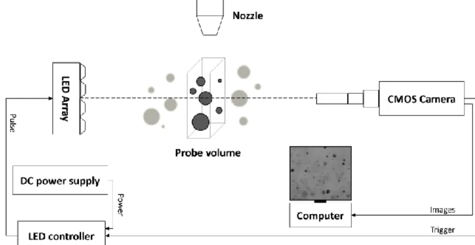
Shadowgraphy involves a backlighted arrangement for image acquisition (Fig. 1). A 8 bit PIV camera (X-Stream™ XS-3, IDT) coupled with high magnification optics provides a working distance of 130 mm. A custom made 72 W LED array (24 Luxeon III Star White LEDs) was placed 500 mm from camera. A LED-controller (PP600F, Gardasoft Vision) provides repeatable intensity control of LED lighting. Shortest pulse duration by illumination system is 1µs. The controller is synchronised using the camera external trigger.

Fig. 1. Backlighted image acquisition set up.

Image Processing Method

Image acquisition

Digital images are 1024 × 1280 with pixel values ranging from 0 to 255 according to the local light intensity. Drops appear on images as a darker region on a brighter background.

Two consecutive images are acquired within a very short time thanks to the double exposure mode of the PIV camera. Image exposure time and delay between the two images are determined by the width and delay of the light pulses respectively. The delay between the two images determines the dynamic range for drop velocity measurement. The image acquisition is followed by the image processing which has the objective to determine the size and the velocity of the drops (Fig. 2).

Drop sizing algorithm

Drop tracking principle

Fig. 2. Flow chart of the drop sizing algorithm (left). Drop tracking principle using a search area based on a priori knowledge of the flow direction in order to retrieve the same drop on two successive frames (right).

Background correction

Spatial illumination heterogeneity correction consists of subtracting the background from each image. Background can be acquired by two means: record an image without any drop on the field of view or recompose it from few acquired images. In this last case, the application of a rank order filter on a set of recorded images provides a good background approximation. The composite background is then generated from the 80 percentile of each pixel intensity on a set of 50 images. Finally, in order to maximize the image contrast independently from the conditions of acquisition, the grey level is rescaled such that 1% of pixels are saturated (i.e. equal to 0 or 255).

Drop localisation

As drops shadow present variable grey level depending on drop size, degree of focus and local illumination, there is no unique threshold adapted for an accurate segmentation of all objects. Therefore, each drop is analysed individually in order to take into account local image context. The first localization of the drops is achieved by computing the light intensity gradient on whole image. Drops smaller than 5 pixels or truncated by the edge of the image are rejected because of the weak measurement accuracy. Centroid coordinates are computed for the retained objects, which are isolated in sub-images for the subsequent individual sizing.

Drop sizing

Segmentation of sub-images is realised by the Canny edge detector (Canny, 1986). This method finds object edges from the local gradient maxima. It provides a 1 pixel thin continuous response

corresponding to highest values of local gradient. Making the hypothesis that this response corresponds to drop shadow boundaries, drop size is determined by computing the inner area defined by the edge.

Out of focus drops rejection

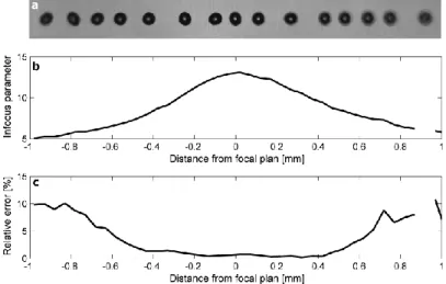
Rejection of out of focus drops is essential for an accurate drop sizing. Drop degree of focus is related to the drop distance to the focal plan. Selection of drops with a minimal degree of focus determines the depth of field measurement and, consequently, the measuring sampling volume. A well-focused drop exhibits a sharp transition with the background at its boundaries (Fig. 3a), while the degree of focus decreases as a drop moves away from the focal plan and a larger grey halo appears around the object (Fig. 3b and c).

Fig. 3. Gradient distribution for a transect across three synthetic drop shadows with decreasing levels of sharpness (a: sharp, c: blurred).

Fig. 4. Oblique shoot of 350 µm drops stream (a). In-focus parameter (b) and relative error on the measurement (c) in respect with the distance from focal plan.

Gradient intensities at drop boundaries increase with drop degree of focus. According to this observation, a focus parameter adapted from the in-focus parameter of Lecuona is proposed:

. . back object bound I I grad parameter Focus  

where gradbound is the mean intensity gradient value at the drop boundaries, Iobject and Iback are grey levels of the drop and the background, respectively.

To avoid the effect of noise or of the bright spot caused by light scattering, Iobject and Iback are computed with a rank order filter such as the median value. This parameter is robust to local illumination variations since it is based on the contrast between the object and the local background.

Thresholds for focused drop selection were determined by studying the evolution of the focus parameter and the error on drop size measurement from images containing drops of known size at various distance of the focal plane (Fig. 4 a). This is achieved using a custom-made drop generator that produces a chain of equally spaced and monosized drops by stimulation of Rayleigh-Plateau break-up (Sirignano & Mehring, 2000). The drop chain is shot with angle of 75° with respect to the optical axis. Focus parameter thresholds were then chosen to result in an error lower than 5% on measured diameters (Fig. 4b and c). The measurement error estimation uses a reference diameter computed from the following relationship:

3 6 f Q d  

where d is the droplet diameter [m], Q is the flow rate measured by bucket method [m³/s] and f droplet generation frequency [Hz] which is known from the mono-sized generator method.

Particle Tracking Velocimetry (PTV)

Drops are tracked between image pairs for velocity computing. Several criteria are required to identify the same drop on two successive frames with a high level of confidence. The most evident criterion is the conservation of drop diameter. The second criterion is the displacement expected between two frames. In an agricultural spray the mean drop direction is known, providing a hypothetic localisation of a drop on the second exposure. In this algorithm, the search area on the second frame was defined as a circular sector oriented along the mean flow direction (Fig. 2b). The opening angle θ is defined as the maximum angle between the main flow direction and a particle displacement, depending on turbulence intensity. Maximal displacement of a particle between two frames is determined according to the delay between the two exposures and a maximal velocity assumption for the spray:

t v

d_max  _max

where dmax is the maximal displacement [m], vmax is the maximal velocity [m.s-1] and Δt is the delay between the two exposures [s].

An adapted definition of the search area is essential for the proper functioning of the PTV algorithm. Indeed, a too big search area will lead to possible mismatches of drops and finally in an error on the computed velocity. Inversely, too restrictive criteria will limit the drop pair matching to slow drops and result to a biased measurement of the drop size distribution due to the non-detection of faster drop.

Drop size distribution correction

All the drops do not have an equal sampling probability because of the sampling method. Sampling probability is governed both by the size of the probe volume and the residence time of drops into this volume, which depends on drops velocity and size. A slow drop remains in the probe volume for a longer time, therefore has more probability to be recorded in the subsequent frame than a faster one (Fig. 5).

Fig. 5. Corrected field of view (FOVCOR, doted box) depending on the drop size and velocity. A drop cannot be cropped by the image edge and has to appear on the second image. The corrected field of view is defined as the area on the first image wherein the drop must appear to be measured.

The larger the drop is, the higher the probability to touch the image edges and to be rejected. Drop size distribution is then established by weighting the volumetric contribution of accepted drop by a correcting factor (CF), which is defined as follow for drops crossing the image lengthwise:



_







v

FOV

DOF

CF

where v is the drop velocity [m.s-1], DOF is the camera depth of field depending on drop diameter [m] and FOVCOR is the corrected camera field of view [m²], which is the image area in which a drop must be in the first acquisition to be measured (Fig. 7) and is determined as follow:



 











FOV_COR      

where L and w are the length and the width of the image respectively [m], D is the drop diameter [m] and Δt is the delay between two exposures [s]. This parameter is computed making the assumption that the drop velocity is mostly vertical, which means that the algorithm does not take into account the possible exit of a drop from the side of the image.

Image processing implementation

Matlab R2011a with image processing toolbox was chosen as technical computing language to implement the above image processing and analysis. The Matlab routines are available at the permanent URL: http://hdl.handle.net/2268/150929.

Experiment conditions

Simultaneous measurements were performed in a tap water flat fan spray produced by a Teejet TP

11001 set at 4.5 bars. The probe volume of both a commercial 2-D PDA (TSI) and shadowgraphy

were localized 50cm below the nozzle in the centre of the spray.

Results and Discussion

Fig. 6 presents the relative cumulative volume curves using the two measurement methods. The curves are similar but present different slopes.

Table 1. Teejet 11001 Spray parameters measured with PDA and shadowgraphy at 50cm below the nozzle PDA Shadowgraphy Dv10 [µm] 91,5 73,8 Dv50 [µm] 132,4 124,3 Dv90 [µm] 178,0 202,1

Relative Span Factor 0,665 1,033

Number of drops 71 999 39 815

Table 1 presents spray parameters measured with the PDA and the shadowgraphy method. Dv10, Dv50 and Dv90 are the drop diameters in respect of which 10%, 50% or 90% of the spray volume are respectively smaller. Relative span factor that characterize the drop diameter dispersion is computed as (Dv90-Dv10)/Dv50. The Dv50 presents a 12 µm discrepancy between the two methods, a difference magnitude often observed when spray drop size measurement methods are compared. The shadowgraphy method presents a bigger span corresponding to a wider drop size distribution. However, the order of magnitude of the span of hydraulic nozzle is often close to one. This parameter is very sensitive to various parameters and associated corrections that are performed for the two measurement methods. The PDA is known to correct the relative proportion of smaller drops taking into account the theoretical smaller sampling volume on one side. On the other side, the shadowgraphy is corrected using the droplet speed measurements, what increases the proportion of bigger drops as they are faster to get an estimation of flux density. This last correction drastically increases the span factor.

Conclusions

A routine implemented in a general technical computing language was developed on the basis of established image processing techniques. This low-cost backlighted imaging technique was tested as an alternative to established optical techniques for characterizing agricultural spray quality. Shadowgraphy offers high contrasted images suited for drop edge detection. The use of local sub-images overcomes contrast heterogeneity issues and the focus parameter ensures accurate drop sizing and localization. The focus parameter threshold was calibrated using a drop generator producing an oblique monosized drop stream within the focal plane. A correction of drop size distribution was required since the technique is volumetric. This was achieved by weighting the volumetric contribution of accepted drops by a correcting factor mainly depending on drop diameter and velocity. The values of criteria used in the tracking algorithm were tuned to avoid drop mismatching leading to improbable measured drop velocities. Information about spray characteristic such as DV10, DV50, DV90 and relative span factor are extracted after a fully automated treatment of digital images.

Comparison of this technique to commercial PDA has been performed by simultaneous measurement at the same measurement point. The results showed good agreement between both techniques. Discrepancies are in the usual range observed amongst drop sizing methods. Given the absence of an absolute reference technique for drop size distribution, any true validation of the shadowgraphy technique is feasible. Therefore, further work will assess the technique capability to distinguish the nozzle BCPC categories by characterizing reference nozzles.

Acknowledgements

The authors would like to thanks Dr David Nuyttens and Donald Dekeyser from the Institute for Agricultural and Fisheries Research (ILVO), Merelbeke, Belgium for the PDA measurements.

References

Canny J. 1986. A computational approach to edge detection. IEEE Transactions on Pattern

Analysis and Machine Intelligence 8:679–698.

Cousin J, Berlemont A, Ménard T, Grout S. 2012. Primary breakup simulation of a liquid jet

discharged by a low-pressure compound nozzle. Computers and Fluids 63:165–173.

Hirleman D, Bachalo W, Felton P. 1990. Liquid Particle Size Measurement Techniques, 2nd

Edition, ASTM STP 1083, American Society for Testing and Materials, Philadelphia.

Lecuona A, Sosa P, Rodríguez P, Zequeira I. 2000. Volumetric characterization of dispersed

two-phase flows by digital image analysis. Measurement Science and Technology 11:1152–1161.

Massinon M, Lebeau F. 2012. Experimental method for the assessment of agricultural spray

retention based on high-speed imaging of drop impact on a synthetic superhydrophobic surface.

Biosystems Engineering 112:56–64.

Sirignano W, Mehring C. 2000. Review of theory of distortion and disintegration of liquid