Modeling multilayered wire strands, a strategy based on 3D finite element beam-to-beam contacts - Part I: Model formulation and validation

1

Modeling multilayered wire strands, a strategy based on 3D finite element

beam contacts - Part I: Model formulation and validation

3

Sébastien Lalondea, Raynald Guilbaultb, Frédéric Légeronc 4

a

Université de Sherbrooke, Faculty of Engineering, Department of Civil Engineering, Sherbrooke, Canada 5

b _{École de technologie supérieure, Department of Mechanical Engineering, Montreal, Canada} 6

c _{Parsons Corporation, Abu Dhabi, United Arab Emirates} 7

8

Abstract

9

This paper proposes a FE modeling strategy for multilayered strands subjected to multiaxial loads. The approach takes 10

advantage of beam elements and incorporates 3D inter-wire contacts. While reducing mesh sizes, it handles any strand 11

configuration. Comparisons with experimental results validate its precision. The analysis shows that friction forces control 12

the hysteresis and the bending stiffness. The paper develops a multi-level friction coefficient better representing the stick 13

and slip zones, and to account for indentation, the model incorporates a friction orthogonality concept; the axial direction is 14

controlled by adhesion, while the orthogonal direction is associated with adhesion and deformation contributions. 15

Keywords: Multilayered wire strands, Finite element modeling, Bending loads, Inter-wire contact, Beam-to-beam contact, Frictional contact 16

17

1. Introduction

18

Multilayered helical strands are key components in many engineering structures, such as suspension and cable-stayed 19

bridges, guyed towers, and power transmission lines. Mainly designed to support high axial static forces, strands are also 20

subjected to dynamic transverse loads (such as wind-induced vibrations) generating free cyclic bending. Near restrained 21

terminations, cyclic bending may induce critical fretting damage at inter-wire contact interfaces, consequently affecting cable 22

service life [1,2]. Characterizing and understanding the mechanical behavior of helical strands under multiaxial loading is thus 23

critical for the structural integrity assessment of engineering structures. This paper develops an efficient modeling strategy 24

for multilayered strands submitted to combined axial and bending loads. Although not restricted to, the proposed modeling 25

approach is oriented to the analysis of overhead conductors. 26

Due to contact interactions between wires, multilayered strands (Fig. 1a) exhibit a variable bending stiffness (EI); as the 27

strand curvature (κ) increases, the wires progressively start to slip on each other, resulting in a significant reduction of the 28

bending stiffness. Therefore, particularly as a result of the anti-symmetricity of the problem [3], formulating a mechanical 29

model of helical strands submitted to multiaxial loads, including bending moments, represents a difficult task. 30

Several models in the literature address the bending of helical strands. Based on the strand load/deformation 31

configuration in Fig. 1a, different theoretical approaches are proposed using various kinematic assumptions [3]. For example, 32

2 Raoof and Hobbs [4] idealized the strand as a series of concentric orthotropic cylinders, each associated with a specific layer 33

and its corresponding mechanical properties. Lanteigne [5] presented a modeling approach in which the strand response is 34

mainly defined from wire axial forces and independent wire bending. Leclair and Costello [6] applied the Love curved rod 35

equilibrium equations to each wire to derive a mechanical model. 36

The literature also proposes analytical models focusing on local wire aspects. For example, Argatov [7] analyzed the 37

influence of transverse modifications of the wire section associated with Poisson ratio effects and inter-wire contact 38

flattening. The study revealed that for larger lay angles the contact flattening effects dominate the influence of the Poisson 39

ratio. Later Frikha et al. [8] used an asymptotic expansion approach and exploited the translational invariance of single wires 40

to reduce the dimension of the elastic problem brought in by helical strands. They were therefore able to describe the micro 41

stresses resulting from macroscopic loadings. Although, the analytical models developed in these studies provide detailed 42

descriptions of strand response, the presented analyses remained limited to axial loads and neglected inter-wire friction 43

forces. 44

Some researchers introduced wire slippage by means of the Coulomb friction law, considering interlayer pressure and 45

axial tension difference in contacting wires at given strand curvatures. This procedure results in a stepwise variation of the 46

bending stiffness between two extremes: EImax (no slip, eq. (1.1)) and EImin (full slip, eq. (1.2)) [9]. In eqs. 1.1 and 1.2, Ej, Aj, γj

47

and Rj stand for wire j elastic modulus, cross-section area, angular position and corresponding layer radius, respectively,

48

while I0j is the wire moment of inertia (relative to its own axis):

49

 









The EImax assumption considers that all strand wires act together as a solid beam, while EImin supposes independent

52

responses of the wires. In other words EImin supposes that each wire bends about its own axis. Therefore, under this second

53

assumption, straight strands involving no inter-wire slip have a bending stiffness equivalent to that resulting from EImax. On

54

the other hand, with bending deformations, the strand curvature generates inter-wire slippage causing bending stiffness 55

reductions. The EImin condition is reached when the induced curvature produces slipping conditions at all wire contacts.

56

In the late ‘90s, Papailiou [10] presented a model in which the friction was also defined by the wire axial tension. The 57

model accounts for the distance from the strand neutral axis, thus leading to a smooth bending stiffness variation between 58

EImax and EImin. To incorporate EI variations along the strand under free bending conditions, the approach was implemented

3 into a finite element analysis. Comparisons with experimental measures showed good correlations [10]. Subsequently, Hong 60

et al. [11] reconsidered certain hypotheses related to pressure transmission between layers, while Paradis and Legeron [12] 61

extended the representation to include the effects of tangential compliance at contact interfaces. 62

Despite the good performances more recent models have shown in predicting strand-free bending response, their 63

analytical formulations involve significant simplifications [13]. For instance, contacts between adjacent wires on the same 64

layer are neglected, while contact points of superposed layers are replaced by contact lines. Moreover, under no-slip 65

conditions (EImax), strand cross-sections remain plane after bending (Euler-Bernouilli hypothesis) [11]. The wire torsional

66

stiffness is also neglected. These hypotheses are acceptable for global analyses of strand located far from restrained 67

terminations. However, they may induce significant deviations when evaluating wire stresses close to positions where fatigue 68

damage is a primary concern. Moreover, due to the inherent limitations of closed-form analytic models, considering the 69

effects of restraining fixtures (suspension clamps) and analyses beyond the material linear elastic limits are practically 70

impossible. 71

To overcome the limitations of analytical models, and mostly as a result of recent advances in numerical methods and 72

computer performance, several authors have proposed full 3D finite element modeling [14–17]. In these numerical studies, 73

each wire of the multilayered strand is discretized with 3D solid elements, where surface-to-surface contact elements 74

simulate all inter-wire contact types. In some cases, the model accounts for plastic deformations by means of nonlinear 75

hardening laws [14,15]. With the ability to characterize local wire stresses without losing the global strand kinematics, 3D FE 76

models appear to be very useful. However, the full 3D solid modelling approaches inevitably generate models leading to high 77

computational cost [14,18]. This in part explains why 3D FE strand models are almost exclusively limited to short-strand-78

length, and axi-symmetrical loads (axial tension and torsion). Although Zhang et al. [19] successfully analyzed strand bending 79

stiffness using a solid 3D FE model, their study was considering a single layer cable of one pitch length. 80

In reality, to minimize boundary effects, multilayered strand analysis under free bending conditions would require a 81

model capable of supporting long spans of few pitch length. Unfortunately, current FE models still appear to be inadequate 82

when it comes to efficiently analyzing the free bending of multilayered strands. 83

This paper develops an intermediate FE modeling approach. The objective is to obtain a precise model eliminating most 84

of the simplifying hypotheses of theoretical models, while remaining computationally affordable. The proposed approach 85

4 uses 3D one-dimensional elements known as beam elements, combined to a beam-to-beam contact algorithm to describe 86

wire geometry and contact interactions. 87

The beam elements strategy has recently been evaluated in some papers [20,21]. Zhou and Tian [21] used beam elements 88

to model a single-layered strand, where the wire contact interactions were managed through coupling equations between 89

correspondent nodes. Inter-wire slippages were therefore not considered, and even though the model was applied to 90

analyses of strands submitted to bending loads, this approach remains limited to single-layered strands under small 91

deflection. In Beleznai et al.’s [20] paper, each inter-wire contact is simulated by spring elements presenting a stiffness 92

derived from Hertz contact theory. Although the accuracy of the approach was demonstrated, the authors acknowledge that 93

it remains limited to one- or two-layered strands submitted to small displacements. 94

The present paper extends the beam modeling approach to multilayered strands undergoing large deformations and 95

displacements. Although the developed procedure is general and appropriate for any finite element (FE) software, this work 96

uses Ansys®. 97

98 99

2. Finite element modeling approach

100

2.1. Multilayered wire strand geometry 101

Generally, wire strands are composed of N helical layers wrapped around a straight central core. Adjacent layers are usually 102

wound in opposite directions to minimize internal moments due to winding effects (Fig. 1b). Each layer i is characterized by 103

the number of wires (ni), the wire diameter (dj), its lay angle (αi) and its layer radius (Ri) given by eq. (2.1):

104 k=i-1 core i i k k=1

d

d

R =

+ +

d

2

2



Since, in the proposed approach, the 3D beam element nodes are located on the wire axis, the whole strand geometry is 106

completely defined by the wire centerlines. For straight cable segments, the wire centerlines are helix curves (Fig. 1c). 107

Following an approach similar to Stanova et al. [16], the helix curve of wire j in a layer i is generated from parameterized 108

equations (eq. (2.2)):, 109

5









where t ϵ [0,1], L is the strand length, q determines the right hand (q = 1) or left hand (q = -1) lay direction, and θi is the total

112

rotation i given by θi = tan(i)L/Ri. Finally, γi is the wire starting angular position (Fig. 1b).

113 114

2.2. Geometry discretization 115

Each wire centerline is discretized using one-dimensional 3D beam elements (Fig. 1c). The BEAM189 elements in Ansys® 116

are composed of three nodes with 6 degrees of freedom (DOF), and use second-order shape functions. The beam element 117

stiffness matrices are defined in the linear elastic domain via the wire radius (r), the material Young modulus (E) and Poisson 118

ratio (υ). In reality, the present work does not integrate the υ effects on the transverse contractions of the wire sections; 119

indeed, Ghoreishi et al. [22] demonstrated that for lay angles (α) below 15° these deformations only have a negligible 120

influence on the global strand behavior. Kumar and Botsis [23] also concluded that υ induces no significant alteration of the 121

contact stress distributions in multilayered strands. 122

As illustrated in Fig. 1c, the beam elements reduce the mesh size by 2 orders as compared to 3D solid modeling. 123

Obviously, this approach cannot account for local form deviations. However, based on St-Venant principle, it may be 124

considered that these local effects should not affect the macroscopic behavior of the global wire strand. 125 126 T, ε Mt, φ Mb, κ ρ Ri i Core Layer i y x γi a) b) wire central helix curves 3 nodes beam element x y z c) 127

Fig. 1 – Wire strand load/deformation configuration (a), geometric configuration (b) and FE model using beam elements (c)

128 129

6 2.3. Inter-wire contact modeling

130

Interactions between wires represent one of the key aspects of wire strand characterization. Two types of contacts can 131

be found in a strand: 1- Lateral contacts (Fig. 2a) correspond to the interactions between wires of the same layer, while 2- 132

Radial contacts associate wires of adjacent layers (Fig. 2b). Contacts between the central core and adjacent layers belong to 133

the Lateral contact category. 134

αi

αi -1

Δx

radial contacts distribution strand axis b) αi+ αi -1 x2 x1 a) ri-1 ri l master elem. (elem. targe170) slave nodes (elem. conta176) n ri ri lj lk li master elem. (elem. targe170) slave nodes (elem. conta176) 135

Fig. 2 – (a) Lateral contact line and (b) radial contact point with 3D beam-to-beam contact configuration

136

A line-to-line contact approach using one-dimensional 3D master/slave element contact pairs, mapped onto beam elements 137

(Fig. 2) is employed for both inter-wire contact types. In Ansys®, contact elements CONTA176 and TARGE170 constitute the 138

slave and master elements, respectively. For radial contacts, CONTA176 elements are mapped onto beams of the inner layer, 139

while TARGE170 elements are associated with the elements of the second layer. The occurrence of contact between two 140

beam elements is determined using a gap function (gn) (eq. (2.3)); contact interactions are established when gn ≤ 0:

141





n i i+1

g = l - r +r (2.3)

142

In eq. (2.3), I represents the normal distance between the centerline of contacting beam elements (Fig. 2(a)). Moreover, 143

since the line-to-line contact algorithm integrated in the present solution neglects the wire flattening and radial contraction 144

contributions, the wire cross-sections are assumed to have constant radii ri and ri+1.

145

For parallel wires (Lateral contact), contact conditions (open or closed) are verified at each contact node, while for crossing 146

wires (Radial contact), the conditions are evaluated all along the length of the beam elements. In the present model, each 147

inter-wire contact is individually defined by a set of master/slave element pairs. For lateral contact, all the beam elements 148

associated with the considered wires are included in the contact pair. On the other hand, for radial contacts, only elements 149

near the contact point are examined. To select the proper beam elements, the location of each radial contact point 150

(illustrated in Fig. 2b) is estimated using the relation defined by eq. (2.4) [24]: 151

7

 





 



cos α

2πR

x

n

sin α +α

where Rct is the contact radius between layers i and i-1, given by Rct = Ri - di/2 = Ri-1 + di-1/2.

153

The proposed model also accounts for friction at inter-wire contacts. Based on Coulomb frictional law, when juxtaposing 154

normal (P) and tangential (Q) inter-wire contact forces obtained from the FE solution, the wires are assumed to be under 155

stick conditions when |Q| ≤ μP and to start slipping when |Q| reaches μP. Thus, under the sticking condition no relative 156

tangential wire displacement is allowed at the contact interface. On the other hand, under the sliding condition the 157

contacting wires slide on each other and |Q| is set to μP. 158

While various contact algorithms are available for modeling contact pairs, the penalty method is preferred because of the 159

large number of inter-wire contacts involved, and because it does not add any DOF to the equation system. The penalty 160

algorithm uses a normal (Kn) and tangential (Kt) contact stiffnesses in order to minimize the penetration (δn) and prevent

161

relative sliding (δt) in stick conditions at the contact and interface. Ansys® defines these parameters with the following

semi-162

empirical expressions (eq. (2.5) and eq. (2.6)): 163 n n K n

K = f

  

E d ξ

f

μ E d ξ

K =

h

  



where in eq.(2.5) fKn is a normal stiffness factor, d the beam element diameter, and ξn a multiplying factor whose default

166

value is set to 10. In eq. (2.6) fKt is a tangential stiffness factor, h the contact element size, and ξt a multiplying factor set to

167

3.75 by default. Values of 1.0 and 50.0 for fKn and fKt respectively, have proven to give results comparable to the Lagrangian

168

contact algorithm commonly considered as theoretically exact. 169

170

2.4. Boundary conditions and loading application 171

In order to prevent any wire unwinding displacement, the ends of the strand are considered as rigid planes. Thus, all 172

nodes located at one strand extremity are fully coupled to the node located at the central core by constraint equations. The 173

end boundary conditions (traction force, imposed extension or displacement constraints) are thus applied only at the central 174

core nodes. 175

8 2.5. Model solution

177

The wire strand model solution makes use of a direct sparse solver, combined to a Newton-Raphson algorithm to deal 178

with large displacements, contacts and material nonlinearities. Force and moment equilibrium are verified at each solving 179

iteration where convergence is assumed when the L2 norm residual is less than 0.5%. All simulations presented in this paper 180

were realized on a 2.9 GHz quad-core CPU with 12 GB of RAM. 181

182

3. Model validation

183

This section establishes the precision of the proposed approach. Results of published studies are compared to values 184

obtained from the present model. 185

3.1. Wire strand analysis under axial loading 186

Fig. 3 shows the first examined configuration, where the wire strand is submitted to an axial tension load T. 187

L T

188

Fig. 3 - Wire strand cable under axial loading

189

This first analysis considers the 7-wire single layer strand studied experimentally by Utting and Jones [25]. Table 1 presents 190

the geometric and mechanical properties of the strand. Judge et al. [14] recently modeled the same configuration using a full 191

3D FE model made of linear solid elements. The following comparison includes the results of both publications. 192

Table 1 - Properties of 7-wire strand

193

Layer ni di (mm) E (GPa) υ Et (GPa) σy (MPa) αi (⁰)

Core 1 3.94 188 0.3 24.6 1540 -

1 6 3.73 188 0.3 24.6 1540 11.8

194

In the present case, the strand is loaded beyond its elastic limit. The material plasticity is introduced with a bilinear 195

kinematic hardening law using the material yield point (σy) and tangent modulus (Et) given in Table 1. As proposed by Judge

196

et al. [14] the cable model integrates a strand length (L) of 200 mm. The constituent wires are discretized with beam 197

elements with an average length of 10 mm. Preparatory simulations not included here showed good convergence/CPU time 198

ratios with this mesh definition for the wire diameter (dj) ranging between 3 and 5 mm. This element size is thus used for all

199

following simulations. The 7-wire single layer strand mesh includes 168 beam elements, 288 contact pairs and 343 nodes. 200

9 Compared to the 147,000 solid elements and 163,212 nodes of the full 3D reference model [14], the proposed approach 201

offers an obvious mesh size reduction. Although not specified in the work of Utting and Jones [25], Judge et al. [14] applied a 202

friction coefficient μ of 0.115 to all contact points. The present simulation uses the same coefficient value. 203

The strand analysis integrates fixed and free end boundary conditions. The fixed end condition only admits axial 204

extensions, while the free end one also permits rotation about the strand axis. Fig. 4 compares the calculated axial 205

load/deformation results to the published experimental and numerical values. 206 207 0 30 60 90 120 150 0,000 0,003 0,006 0,009 0,012 0,015 A xi al lo ad (kN )

Strand axial strain

Exp. fixed end [25] Full 3D model fixed end [14] Present model fixed end Exp. free end [25] Full 3D model free end [14] Present model free end

208

Fig. 4 - Axial strain vs. axial load for the 7-wire strand

209

Fig. 4 shows the high correspondence between the results established with the proposed modeling strategy and those 210

published in the references. 211

The same case study was also modeled by Jiang and Henshall [26]. Exploiting the cyclic symmetry of the strand, the 212

authors developed a refined 3D FE model including only one wire and the contacting core sector. This approach produced 213

detailed information on the contact stresses. Table 2 compares the inter-wire contact forces per unit of length (p) extracted 214

from the present model to those presented by Jiang and Henshall [26]. The table indicates that the overall correspondence is 215

higher than 93%. 216

Table 2 – Core-wire contact force comparison

217 Axial Strain (ε) p (N/mm) Ref. [26] p (N/mm)

Present model Diff. (%)

0.002 40.3 43.0 6.6 0.004 80.8 85.9 6.2 0.006 120.8 127.9 5.9 0.008 160.4 169.9 5.9 0.010 178.7 185.3 3.7 0.012 184.7 189.9 2.8 218

In addition to the 7-wire strand, Judge et al. [14] also examined a 120-wire multilayered steel strand. Table 3 gives the 219

120-wire strand properties taken from the reference paper. The authors of the paper established the tangent modulus Et

220

from the wire axial stress/deformation chart [27]. 221

10 Fig. 5a shows the stress distribution established with the present model, while Fig. 5b compares the axial

222

load/deformation results to the values published by Judge et al. [14]. The graph in Fig. 5b also includes experimental data 223

measured on a 6m cable specimen [14]. The reference document [27] indicates that the model solution lasted 12 hours on a 224

desktop computer equipped with quad-core CPU and 32 GB of RAM. 225

Table 3 - Properties of 120-wire multilayered strand

226

Layer ni di (mm) E (GPa) υ Et (GPa) σy (MPa) αi (⁰)

Core 1 5.8 188 0.3 5.5 1540 - 1 7 4.3 188 0.3 5.5 1540 11.94 2 17 3.2 188 0.3 5.5 1540 14.75 3 14 5.3 188 0.3 5.5 1540 14.37 4 21 5.0 188 0.3 5.5 1540 15.23 5 27 5.0 188 0.3 5.5 1540 15.66 6 33 5.0 188 0.3 5.5 1540 15.95 227

The full 3D model required 2,520,000 solid elements and 2,797,920 nodes for a length L equal to 200 mm [14]. On the other 228

hand, the present approach led to a mesh size of 2640 beam elements, 5869 contact pairs, 5400 nodes and a 62-minute 229 solution. 230 231 1300 (MPa) 750 200 475 1025 a) 0 1 000 2 000 3 000 4 000 0,00 0,01 0,02 0,03 0,04 0,05 0,06 0,07 Ax ia l Lo a d ( kN )

Strand axial strain (εa)

b)

Nominal axial stiffness Exp. [14] Full 3D model [14] Present model

232

Fig. 5 - 120-wire strand partial view of Von Mises stress (σVM) distribution at (a) εa = 0.0056 and (b) axial strain (εa) vs. axial load

233 234

Although the numerical solutions significantly deviate from the experimental measures for the elastic domain part, Fig. 5b 235

shows that both models produce valuable and similar predictions of the theoretical cable stiffness. Judge et al. did not 236

explain the experimental/numerical differences. 237

These first results show that, while considerably reducing the mesh size, the proposed beam modeling strategy offers 238

descriptions of the global behavior of axially loaded strand cables with a precision equivalent to that provided by significantly 239

more sophisticated models, and even extends beyond the elastic limit. 240

241 242

11 3.2. Strand response under combined axial/bending loads

243 244

This second series of validation analyses combines bending forces and axial loadings. Fig. 6 illustrates the cable load 245

arrangement. This configuration corresponds to the experimental bending tests conducted by Papailiou [10,28], where a 246

transverse load V varying between 0 and Vmax is applied at the midspan position (z = 0 mm), while the wire strand is

247

maintained at a specified tension value T, using rigid clamps. These clamps virtually prevented any cable slippage at both 248 ends. 249 T T V L z y x 250

Fig. 6 - Wire strand cable under axial and bending loading

251

In his work, Papailiou [28] analyzed two multilayered strands: 1- a S32 steel cable (Table 4) and 2- a ACSR Cardinal electrical 252

conductor (Table 5). ACSR strands consist of a steel core and layers of aluminum wires. Both cable specimens were 1.0 m 253

long. 254

Table 4 - Properties of S32 cable

255

Layer Nb. Wire Nb. Wire dj (mm) E (GPa) υ α (⁰)

Core 1 3.72 200 0.3 - 1 6 3.54 180 0.3 14.22 2 12 3.54 180 0.3 13.69 3 18 3.54 180 0.3 13.99 4 24 3.54 180 0.3 13.97 256

Table 5 - Properties of Cardinal ACSR conductor

257

Layer Nb. Wire Nb. Wire dj (mm) E (GPa) υ α (⁰)

Core 1 3.34 210 0.3 - 1 6 3.34 180 0.3 6.06 2 12 3.32 65 0.33 11.99 3 18 3.32 65 0.33 11.80 4 24 3.32 65 0.33 13.10 258

The following section examines the S32 cable. The present analysis assumes a linear elastic behavior, and imposes a constant 259

coefficient of friction a equal to 0.3 for all inter-wire contacts. This value is derived from friction force measurements

260

published by Papailiou [28]. The DOF of both cable ends are constrained and only admit displacements in the axial direction. 261

In addition, to prevent any rigid body movement, one core node located at the cable midspan (z = 0 mm) is axially 262

constrained. The modeled cable length is L = 1000 mm. This length corresponds to the reference experimental test setup 263

[10]. 264

12 During the first load steps, the tension force T is applied in 20-load increments, and thereafter maintained for the rest of 265

the simulation. After that, the transversal load V is also incrementally applied. After reaching the Vmax value, the transversal

266

load is gradually brought back to 0 following the inverse 20-load steps. This load sequence was repeated for a few load 267

cycles, with T = 280 kN and Vmax = 40 kN.

268

The numerical tests indicated that, using this load configuration, the cable load/deflection hysteresis reaches a steady-269

state regime at the second load cycle. 270

Fig. 7a shows the strand deformation and corresponding von Mises stress distributions after two load cycles, while Fig. 7b 271

presents the resulting midspan load-deflection curve. The graph of Fig. 7b also includes Papailiou's experimental 272

measurements and the theoretical evaluations made with eq. (3.1), considering EImax and EImin.

273

In eq. 3.1, k = (EI/T)½ and s = L/4. Integrating the S32 cable properties given in Table 4 into eqs. 1.1 and 1.2 leads to 6357.8 274

Nm² and 82.7 Nm² for EImax and EImin, respectively.

275

The experimental and theoretical evaluations presented in Fig. 7 have been shifted to have their origins correspond to the 276

x-intercept of the steady-state hysteresis. 277 -L 2k max -L 2k Vk L 1- e y = -T 4k 1+ e       (3.1) 278

While the chart shows a good correlation between the model predictions and the experimental data, the large hysteresis 279

areas indicate that the simulations overestimate the friction losses. 280 0 8000 16000 24000 32000 40000 0 8 16 24 32 40 V ( N ) Deflection (mm) Exp. [28] Present Model EImin EImax b)

Deformed mesh at V = 0 after 2 load cycles Undeformed mesh

4750 (MPa) 2375

0 1188 3563

a)

Deformed mesh at V = Vmaxafter 2 load cycles

281

Fig. 7 - S32 cable (T = 280 kN and Vmax = 40 kN), Von Mises stress (σVM) distributions after (a) 2 load cycles and (b) 5 cycle load-deflection

282

hysteresis curve at the cable center (Z = 0 mm), V variation between 0 and Vmax

283 284

The following simulations consider four load configurations (T;Vmax) given in kN: Case 1 (40;5), Case 2 (80;10), Case 3

285

(140;20) and Case 4 (280;40). Fig. 8 compares the cable deflection over a 150 mm distance to the experimental results 286

13 presented by Papailiou for V = Vmax. The numerical deflection values are evaluated at the nodes defining the central core

287

wire. Moreover, in order to illustrate the wire slippage effect, the graph of Fig. 8 also includes the theoretical cable deflection 288

curves calculated with eq. 3.2 [29], considering the EImax and EImin assumptions.

289

 

y x = sinh - -tanh cosh - 1

2T k k k k            _{ }   _{ }  _{ }        (3.2) 290 291 0 1 2 3 4 0 30 60 90 120 150 D e fle ct io n (m m ) 0 1 2 3 4 0 30 60 90 120 150 D e fle ct io n (m m ) Exp. [28] Present Model a) b) EImax EImin EImax EImin 0 2 4 6 8 0 30 60 90 120 150 D e fle ct ion (m m ) Axial position (mm) 0 1 2 3 4 0 30 60 90 120 150 D e fle ct ion (m m ) c) d) EImax EImin EImax EImin 292

Fig. 8 - S32 cable deflection a) Case 1, b) Case 2, c) Case 3 and d) Case 4

293

The numerical solutions presented in Fig. 8 demonstrate a perfect correspondence with the experimental data. Fig. 8 also 294

illustrates the imprecision associated with the theoretical expression (eq. 3.2). The inaccuracy associated with eqs. 1.1 and 295

1.2 is also visible in Fig. 7b) with ymax.

296

The following analyses examine the ACSR Cardinal conductor described in Table 5. Compared to the previous simulation, 297

the friction coefficient is changed to μa = 0.5 to describe the aluminum-aluminum and steel-aluminum contacts, while μa =

298

0.3 remains at the steel-steel wire contacts. 299

The simulations only include one load case: T = 40 kN and Vmax = 4.3 kN. Fig. 9a) and b) present the cable deflection at

300

Vmax and the midspan (z = 0 mm) load-deflection response, respectively. For clarity, the simulation results established for the

301

first transversal load application have been removed from Fig. 9b), while the remaining part is moved to have its x-intercept 302

at x = 0. Both graphs also include the Papailiou experimental data and the theoretical curves established with EImax = 1800.4

303

Nm² and EImin = 28.3 Nm² (eqs. 1.1 and 1.2).

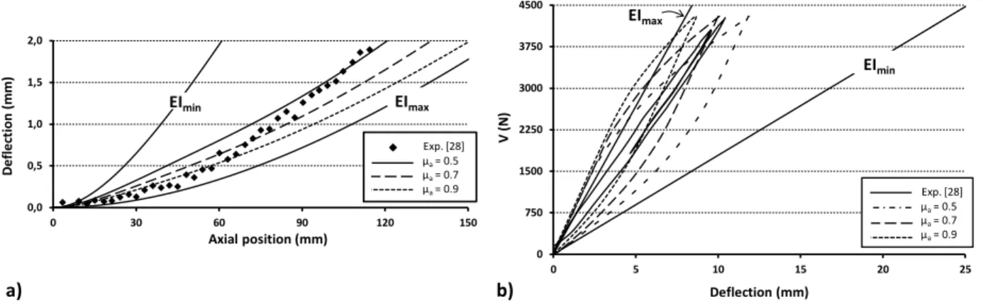
14 0,0 0,5 1,0 1,5 2,0 0 30 60 90 120 150 D ef lec ti o n (mm) Axial position (mm) EImax EImin Exp. [28] Present Model 0 750 1500 2250 3000 3750 4500 0 5 10 15 20 25 V (N ) Deflection (mm) Exp. [28] Present Model EImax EImin b) a) 305

Fig. 9 - ACSR cardinal (T = 40 kN and Vmax = 4.3 kN), (a) deflection and (b) load-deflection curve at the cable center (Z = 0 mm), V

306

variations between 0 and Vmax

307 308

The Vmax deflection comparison once again shows good agreement between the numerical results and the experimental

309

values (Fig. 9a), while the predicted hysteresis area remains larger than the measured response (Fig. 9b). 310

Despite the differences noted, the simulation results show that the proposed modeling approach is adapted to 311

multilayered strand simulation; the model accurately reproduces the nonlinear cable response, which is largely controlled by 312

friction forces at the inter-wire contacts. 313

314

4. Analysis of the wire strand under combined axial/bending loads

315

Although the model capacity to simulate strands submitted to complex loadings was confirmed in the previous section, 316

the differences revealed for the ACSR Cardinal case require additional attention. The following reconsiders the ACSR Cardinal 317

response, and presents a deeper analysis of the Section 3.2 simulation results. 318

319

4.1 Distribution of inter-layer contact interaction 320

Levesque et al. [30] conducted vibration tests on an ASCR Bersfort conductor clamped with fixtures similar to those 321

considered in Papailiou’s research. The tests were conducted with induced vibrations producing deflection amplitudes (Δy) of 322

0.3 mm at 89 mm (3.5 in) from the clamp edge. The authors reported contact point statuses from the first 250mm conductor 323

segment outside the clamp (-500 to -250mm) at layer interfaces 2-3 and 3-4 (see Fig. 12). They mapped the contact 324

conditions according to three statuses: A - Sticking, B – Sliding, and C - Slipping (partial relative displacements). Fig. 10 325

schematically reproduces the reference observations mapped onto the strand. 326

15 0 72 144 216 288 360 -500 -450 -400 -350 -300 -250 -200 -150 A ng ul ar po si ti on (° ) Axial position (mm) TOP BOTTOM NEUTRAL AXIS C A A A A A A A A C A A B B B B B b) 0 72 144 216 288 360 -500 -450 -400 -350 -300 -250 -200 -150 A n gu la r p o si ti o n (° ) TOP BOTTOM NEUTRAL AXIS A A A A A C C C B B B B a) Sticking Sliding Slipping A B C CLAMP EDGE CLAMP EDGE Axial position (mm) 327

Fig. 10 - ACSR Bersfort conductor, mapping of contact points status between (a) layers 2 and 3 and (b) between layers 3 and 4

328

(reproduced from Levesque et al. [30] )

329 330

To assess the validity of the inter-wire contact description obtained from the present model, Fig. 11 presents the model 331

predictions obtained for the ACSR Cardinal conductor defined in Table 5, using a similar mapping approach. In order to have 332

deflection amplitudes comparable to the Levesque et al. [30] test conditions, the tests were conducted with V = 0.4Vmax

333

(Vmax = 4.3 kN).

334

The reference results [30] also revealed slipping marks at the conductor/clamp interface from the clamp edge, up to 22 335

mm inside the clamped zone. In the present model, the node coupling at the conductor ends (equivalent to clamping edges) 336

prevents any relative motion, and can be considered as the limit point of contact slip observed in the reference [30]. Hence, 337

the contact point statuses predicted by the model are mapped in Fig. 11, considering the clamp edge positioned at -478mm 338

(22 mm from the restrained end). Finally, since the model formulation only detects sticking and sliding conditions, and 339

cannot directly describe partial slip, slipping condition occurrences are identified at contact points experiencing a contact 340

status change from sticking to sliding during the V loading process from 0 to 0.4.Vmax.

341 0 72 144 216 288 360 -478 -428 -378 -328 -278 -228 -178 -128 A n gu la r p o si ti o n (° ) Axial position (mm) TOP BOTTOM NEUTRAL AXIS b) 0 72 144 216 288 360 -478 -428 -378 -328 -278 -228 -178 -128 A n gu la r p o si ti o n (° ) Axial position (mm) Sticking Sliding Slipping TOP BOTTOM NEUTRAL AXIS a) CLAMP EDGE CLAMP EDGE 342

Fig. 11 - ACSR Cardinal at V = 0.4Vmax, mapping of contact points status (a) between layers 2 and 3 and (b) between layers 3 and 4

16 A comparison of the numerical results (Fig. 11) to the experimental measures (Fig. 10) shows close similarities, despite 344

the differences between the configurations. Indeed, as indicated in the reference descriptions, the predicted contact 345

mappings show that a majority of the points are under sliding conditions, while sticking and slipping zones tend to 346

concentrate close to the evaluation zone limit (axial position -250 mm) and the clamp edge (axial position -500 mm), 347

respectively. The model produces more slipping points at the layer 2-3 contact interface. However, considering the numerical 348

slipping criterion, some of these contact points would probably have been considered under sliding conditions in the 349

experimental description. Globally, the model establishes interlayer contact interactions which are representative of 350

published experimental observations. 351

352

4.2 - Wire axial force analysis 353

The simulation results presented in Fig. 9 (strand deflection and hysteresis) may also be interpreted through wire axial 354

force (F) distributions. Fig. 13 presents the axial force (F) calculated for the nodes of layers 2 to 4 when V = Vmax

355

(Vmax = 4.3 kN). Fig. 13 also includes the axial force variation (ΔF) established between V = 0 and V = Vmax. Moreover, for

356

clarity, the graphs only include the predictions made for the more descriptive nodes. These nodes are in the regions near the 357

vertical (top and bottom) and horizontal planes shown in Fig. 12. In addition, since the predictions are symmetrical with 358

respect to the central axial position (z = 0 in Fig. 6), the graph only includes the conductor half-length results. The charts also 359

incorporate the deflection curve established when V = Vmax. For all cases, T was fixed at 40 kN.

360 165° - 195° 345° - 15° 75° - 105° (top) 255° - 285° (bottom)

y

x

Fig. 12 – Analyzed conductor layers near vertical and horizontal planes (grayed zones)

17 -500 -400 -300 -200 -100 0 0 3 6 9 12 -500 -400 -300 -200 -100 0 De lf e cti o n (mm) 0 300 600 900 1200 -500 -400 -300 -200 -100 0 F (N ) 0 300 600 900 1200 -500 -400 -300 -200 -100 0 Δ F (N ) -500 -400 -300 -200 -100 0 0 3 6 9 12 -500 -400 -300 -200 -100 0 De lf e cti o n (mm)

Layer 2 Layer 3 Layer 4

a) 75 - 105° 255 - 285° Deflection 0 300 600 900 1200 -500 -400 -300 -200 -100 0 F (N ) -500 -400 -300 -200 -100 0 0 3 6 9 12 -500 -400 -300 -200 -100 0 De lf e cti o n (mm) 0 300 600 900 1200 -500 -400 -300 -200 -100 0 Δ F (N )

Axial position (mm) -500 -400Axial position (mm)-300 -200 -100 0

0 3 6 9 12 -500 -400 -300 -200 -100 0 De lf e cti o n (mm) Axial position (mm)

Layer 2 Layer 3 Layer 4

b)

165 - 195° 345 - 15° Deflection

363

Fig. 13 - Distributions of Fwhen V=Vmax and ΔF for wires of layers 2, 3 and 4 located near the (a) vertical and (b) horizontal planes

364 365

Fig. 13(a) shows that the wires close to the vertical plane experience their maximum F and ΔF values at the V load 366

application points (z = 0mm) and at the clamped end points (z = -500 mm). The charts also indicate that the inner layers 367

support the highest values. F and ΔF are at their minimum amplitude in the straight cable portion (between -150 and -350 368

mm). On the other hand, the wires close to the horizontal plane (Fig. 13b) mainly sustain the axial force peaks in areas 369

between 50 and 100 mm from the mid (z = 0mm) and end (z = 500mm) cable positions. However, the maximum force values 370

remain significantly lower than those close to the vertical plane. Regarding ΔF, the horizontal plane presents a more uniform 371

distribution, although the maximum variations of ΔF remain located at the positions of the force maxima. 372

Because of the strand structure (Fig. 1b), an axial tension provokes tightening displacements of the wires, increasing the 373

contact pressure transmitted to underlying layers. Therefore, the high values of F revealed in Fig. 13a explain in part the 374

sticking statuses observed in Fig. 11 close to the clamp edge location at the top and bottom angular positions (90 and 270 375

degrees). On the other hand, comparing the axial force distribution in the horizontal plane zone angular positions to the 376

contact mappings of Fig. 11 (0-360 and 180 degrees) shows that the highest F/ΔF values are also associated with sticking 377

conditions: between -400 and -128 mm for layer 2-3 contacts and between -328 and -128 mm for layer 3-4 contacts. 378

379

4.2 Inter-wire force analysis 380

The friction wear at a given contact position depends on the local normal force and on the associated sliding distance. 381

This section analyzes the normal force (P), the tangential force (Q) and the slip distance (δ) at selected contact points for the 382

1-2, 2-3 and 3-4 layer combinations. Fig. 14 presents the simulation results at the positions close to the vertical and 383

horizontal planes shown in Fig. 12. The plots of Fig. 14 also include  evaluations made between V = 0 and V = Vmax. Once

384

again, Vmax was 4.3 kN, while the axial tension was kept constant at T = 40 kN.

18 -500 -400 -300 -200 -100 0 0 3 6 9 12 -500 -400 -300 -200 -100 0 D e fle ct io n (m m ) 0 100 200 300 400 -500 -400 -300 -200 -100 0 Pma x (N) 0.00 0.12 0.24 0.36 0.48 -500 -400 -300 -200 -100 0 Δδ (m m ) Axial position (mm) 0.00 0.12 0.24 0.36 0.48 -500 -400 -300 -200 -100 0 δma x (m m ) -500 -400 -300 -200 -100 0 Layers 1-2 0 3 6 9 12 -500 -400 -300 -200 -100 0 D e fle ct io n (m m ) -500 -400 -300 -200 -100 0 Axial position (mm) 0 3 6 9 12 -500 -400 -300 -200 -100 0 D e fle ct io n (m m ) Axial position (mm) Layers 2-3 Layers 3-4 0 100 200 300 400 -500 -400 -300 -200 -100 0 Δ P (N) -500 -400 -300 -200 -100 0 0 3 6 9 12 -500 -400 -300 -200 -100 0 D e fle ct io n (m m ) 0 50 100 150 200 -500 -400 -300 -200 -100 0 Qma x (N) -500 -400 -300 -200 -100 0 0 3 6 9 12 -500 -400 -300 -200 -100 0 D e fle ct io n (m m ) 0 50 100 150 200 -500 -400 -300 -200 -100 0 Δ Q ( N) -500 -400 -300 -200 -100 0 0 3 6 9 12 -500 -400 -300 -200 -100 0 D e fle ct io n (m m ) 75 - 105° 255 - 285° Deflection

Layers 1-2 Layers 2-3 Layers 3-4

-500 -400 -300 -200 -100 0 0.00 0.12 0.24 0.36 0.48 -500 -400 -300 -200 -100 0 δma x (m m ) 0 3 6 9 12 -500 -400 -300 -200 -100 0 D e fle ction ( m m ) 0.00 0.12 0.24 0.36 0.48 -500 -400 -300 -200 -100 0 Δδ (m m ) Axial position (mm) -500 -400 -300 -200 -100 0 Axial position (mm) 0 3 6 9 12 -500 -400 -300 -200 -100 0 D e fle ct io n (m m ) Axial position (mm) 0 100 200 300 400 -500 -400 -300 -200 -100 0 Pma x (N) 0 3 6 9 12 -500 -400 -300 -200 -100 0 D e fle ct io n (m m ) -500 -400 -300 -200 -100 0 0 100 200 300 400 -500 -400 -300 -200 -100 0 Δ P (N) -500 -400 -300 -200 -100 0 0 3 6 9 12 -500 -400 -300 -200 -100 0 D e fle ct io n (m m ) 0 50 100 150 200 -500 -400 -300 -200 -100 0 Qm ax (N ) -500 -400 -300 -200 -100 0 0 3 6 9 12 -500 -400 -300 -200 -100 0 D e fle ct io n (m m ) 0 50 100 150 200 -500 -400 -300 -200 -100 0 Δ Q (N) -500 -400 -300 -200 -100 0 0 3 6 9 12 -500 -400 -300 -200 -100 0 D e fle ct io n (m m ) 165 - 195° 345 - 15° Deflection

a)

b)

Fig. 14 - Distributions of P when V=Vmax, ΔP, Q when V=Vmax, ΔQ, δ when V=Vmax and Δδ for contact points located near the vertical (a)

387

and horizontal (b) planes at layer interfaces 1-2, 2-3 and 3-4

388 389

Fig. 14a) and b) show that, regardless of the horizontal or vertical region considered, the normal (P, ΔP) and tangential (Q, 390

ΔQ) forces are higher at inter-layer 1-2 than at interlayer 2-3 or 3-4. 391

The normal/tangential force combinations generate almost inversely proportional slip displacement δ. For example, Fig. 392

14a shows, for all inter-layer combinations, that the δ predictions remain at low amplitudes for the first 100 mm from the V 393

application point (z = 0 mm) and from the clamp edge position (z = 500 mm). On the other hand, the maximum δ values 394

appear in the 100 to 400 mm portion of the strand; the external layer combination 3-4 show its maximum sliding 395

displacement at 250 mm, which correspond to an inflection point in the conductor deflection curve. 396

The displacement results presented in Fig. 14b for the horizontal plane region show that δ is also minimal at the clamped 397

end, but significant at the V load position. The maximum slip amplitudes are located in the 50-100 mm and 400-450 mm 398

regions, for all three analyzed inter-layers. Globally, compared to the Fig. 14a results, the δ evaluations presented in Fig. 14b 399

19 demonstrate practically inverse amplitude distributions along the strand. Based on the force F, P and Q evaluations, as well 400

as on the slip displacement δ predictions, it may logically be concluded that the wire bulk stress and contact conditions 401

present significant fluctuations along the strand, and that the internal layers are submitted to more severe loading 402

conditions. 403

In addition to the surface wear, the normal force P may also cause immediate plastic contact deformations, and influence 404

the coefficient of friction; normal force augmentation increases real contact areas and, consequently, the associated 405

adhesion coefficient of friction (μa) as well. The tangential force Q and the slip displacement δ also influence the real contact

406

areas and the adhesion coefficient of friction. Therefore, the significant P, Q and δ variations are good indications that the 407

coefficients of friction are not uniform and constant as assumed within the previous simulations. The next section further 408

investigates how the coefficient of friction influences the simulation results. 409

410

5. Friction coefficient influence evaluation

411

Following the previous observations, this section evaluates the effect of different friction modeling approaches. 412

413

5.1 Friction coefficient magnitude effect 414

The influence of μa is first analyzed considering three values for μa at the wire aluminum-aluminum contacts: 0.5, 0.7 and

415

0.9. These coefficients remain similar to the Wharton et al. [31] and Papailiou [10] observations made during experimental 416

fretting/friction tests on aluminum alloy specimens. The contacts involving steel wires remain unchanged and fixed to the 417

values indicated in Section 3.2: μa = 0.3 and 0.5 for the steel-steel and steel-aluminum contacts, respectively. Fig. 15

418

compares the results, and illustrates the influence of μa on the calculated bending deflection.

419

Fig. 15a) particularly shows that increasing μa reduces the deflection slope. Fig. 15b) shows that the high μa and low V

420

combinations lead to higher bending rigidities (EI) than the theoretical upper limit EImax. In reality, the same response may

421

have been produced with the introduction of a higher tangential stiffness (Kt). In other words, a change in the inter-layer

422

friction coefficient may generate a corresponding effect on the bending stiffness. 423

20 0,0 0,5 1,0 1,5 2,0 0 30 60 90 120 150 D e fle ct ion ( mm ) Axial position (mm) Exp. [28] μa= 0.5 μa= 0.7 μa= 0.9 EImax EImin 0 750 1500 2250 3000 3750 4500 0 5 10 15 20 25 V (N ) Deflection (mm) Exp. [28] μa= 0.5 μa= 0.7 μa= 0.9 EImax EImin b) a) 424

Fig. 15 - ACSR Cardinal (T = 40 kN and Vmax = 4.3 kN), (a) deflection and (b) load-deflection curve at the cable center (z = 0 mm) V

425

variations between 0 and Vmax with different values of μa

426 427

The experimental deflection curve shows that close to the V application point (z = 0 mm), the strand deformation 428

presents a lower gradient than at more distant points, suggesting therefore a reduction of the friction coefficient with an 429

augmentation of the distance from the V application point; for z between 0 and 60 mm, the response obtained with μa = 0.9

430

is closer to the measurements, whereas for the remaining part (z between 60 and 120 mm), μa = 0.5 offers a better

431

correspondence. Actually, the experimental result trend remains close to the theoretical approximation EImax up to a distance

432

of 45 mm from the V application point. On the other hand, at greater distances, the experimental deflection never reaches 433

the EImin prediction. In other words, the Papailiou results suggest that the friction behavior remains close to a no-slip

434

condition around the transversal load application point, and progresses toward sliding conditions, while never attaining a full 435

slip state. Since this behavior does dominate the response in the graphs of Fig. 8 (S32 steel cable), it may be assumed that it 436

is mainly controlled by a combination of elastic and plastic localized deformations of the aluminum wires. 437

The hysteresis curves in Fig. 15b indicate that higher values of μa lead to slightly reduced friction losses since more

438

contact points remain under stick conditions. This observation also advocates for high values of μa in the vicinity of the V

439

application. 440

Finally, this analysis indicates that the model should offer an improved precision with friction coefficients better reflecting 441

the variable inter-wire relative displacements along the strand axial position. 442

443

5.2 Variable adhesion friction coefficient effect 444

Considering the mechanical properties of ACSR aluminum wire, it may reasonably be assumed that the loads (P, Q) shown 445

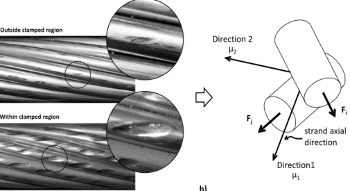
in Section 4 can generate wear and plastic deformations. Fig. 18a shows indentation marks observed on experimental 446

specimens of 19/54 ACSR Géant conductor, similar observations are reported by Azevedo et al. [32]. Altered wire surface 447

21 conditions have a direct effect on inter-wire contact. The influence of wire surface changes may be integrated into variable 448

friction coefficient values. However, predicting the complete distribution of μ along the strand remains an impractical 449

endeavor. The following section examines the response quality improvement resulting from a multi-level adhesion 450

coefficient of friction. 451

In order to force the quasi no-slip condition noted in the V load application point neighborhood and near the clamped 452

ends, a μa value of 0.7, equivalent to a static coefficient, is imposed at aluminum-aluminum and aluminum-steel radial

453

contacts over 100 mm (Lstick) from the V application point (z = 0 mm) and from the strand fixed extremities (z = 500 mm). On

454

the other hand, slip conditions are promoted with a value equivalent to a dynamic coefficient of friction μa = 0.3. This

455

coefficient is applied at the aluminum-aluminum and aluminum-steel radial contacts over four 50 mm strand segments (Lslip)

456

next to the no-slip zone. Fig. 16 shows the proposed μa variations zones. Unaffected strand zones maintain the original

457

coefficient of friction configuration (μa = 0.5 for aluminum-aluminum and aluminum-steel contacts). The steel-steel contact

458

coefficients of friction are fixed at μa = 0.3 throughout.

459 T T V L z y 2Lstick

Lslip Lslip Lslip Lstick

Lslip

Lstick

x

460

Fig. 16 - Two-level coefficient of friction model configuration

461 462

In addition, in order to extend the description of the multi-level coefficient concept, extreme values for μa of 0.9 and 0.1

463

are also evaluated in the stick and sliding zones of the aluminum-aluminum and aluminum-steel contacts. Fig. 17 reproduces 464

the result of Fig. 9 and adds the deflection and hysteresis predictions established for the two aforementioned configurations, 465 introducing variable μa. 466 b) 0,0 0,5 1,0 1,5 2,0 0 30 60 90 120 150 D ef le ct io n ( m m ) Axial position (mm) a) EImax EImin Exp. [28] μa= 0.5 μa= 0.5, μa,stick= 0.7, μa,slip= 0.3 μa= 0.5, μa,stick= 0.9, μa,slip= 0.1 0 750 1500 2250 3000 3750 4500 0 5 10 15 20 25 V ( N ) Deflection (mm) Exp. [28] μa= 0.5 μa= 0.5, μa,stick= 0.7, μa,slip= 0.3 μa= 0.5, μa,stick= 0.9, μa,slip= 0.1 EImax EImin 467

Fig. 17 - ACSR Cardinal (T = 40 kN and Vmax = 4.3 kN), (a) deflection and (b) load-deflection curve at the cable center (z = 0 mm) V

468

variation between 0 and Vmax considering multi-level μa

469 470

22 The curves in the chart of Fig. 17a) show some precision gains realized with the multi-level adhesion coefficient of 471

friction; the predicted deflection better represents experimental data. However, the approach does not significantly 472

influence the friction dissipation; even with the overemphasis brought in with the 0.9 and 0.1 coefficient values, the 473

numerical hysteresis curves presented in Fig. 17b) remain practically unchanged. Therefore, it must be concluded that the 474

multi-zone adhesion coefficient of friction shown in Fig. 16 is not sufficient to explain the experimental observations. 475

476

5.3 Orthogonal friction coefficient effect 477

The previous evaluations only considered the adhesion contribution to friction or μ = μa. The obtained results tend to

478

indicate that this approach is too simplistic, and that a more realistic formulation should incorporate the deformation 479

process. The coefficient of friction (μ) should hence be written as: μ = μa + μd, where μd represents the deformation

480

contribution. Fig. 18(a) shows typical local alterations of wire surfaces caused by contact loads. In addition to adhesion 481

phenomena described by μa, this type of plastic deformation may mechanically constrain the relative displacements of the

482

wires. However, since the proposed FE model does not account for wire cross-section alterations, the deformation 483

contribution cannot be directly integrated. On the other hand, the above μ formulation can easily compensate for this aspect 484

and embody this additional constraint via μd. In reality, the indentation marks generated at the contact points plausibly

485

promote inter-wire slip in a preferred direction. 486

The friction may be defined in orthogonal directions corresponding to the strand axial direction (Direction 1) and the 487

direction (Direction 2) resulting from the cross product between Direction 1 and the normal to the radial contact point (Fig. 488

18b). Direction 1 and Direction 2 do not aim at defining an exact representation of the local indentation mark orientation, 489

but rather, it is to provide a global representation of the strand assembly. The coefficients of friction μ1 and μ2 represent

490

Directions 1 and 2, respectively. These coefficients are expressed as μi = μai + μdi.

491

The expression of the coefficient of friction may be reduced to a unique function of μa: μi = μai(1+cdi), where the constant

492

cdi represents the deformation contribution. Moreover, considering μa2 = μa1, the relation between μ1 and μ2 may be defined

493

by the ratio μ2/μ1 = (1+cd2)/(1+cd1). As well, assuming that Direction 1 is controlled by adhesive bonds, cd1 may be set to zero.

494

The μ2/μ1 value is then reduced to (1 + cd2).

495

In the model, μ1 and μ2 are independent parameters. Hence, setting μ2 to zero would isolate the adhesion contribution,

496

whereas setting μ1 to zero would emphasize the friction caused by the deformations.

23 To illustrate the influence of the orthogonal friction concept, the following section re-evaluates the ACSR Cardinal

498

response when cd2 is set to 0, 4, 9 and 14, which leads to the corresponding μ2/μ1 ratios 1, 5, 10 and 15, respectively. Fig. 19

499

presents the simulation results established for these ratios when the aluminum-aluminum μa values are 0.5, 0.7 and 0.9. The

500

coefficients of friction at the steel-steel and steel-aluminum contacts were maintained at 0.3 and 0.5, respectively. 501 502 Fi Fj Direction 2 μ2 Direction1 μ1 strand axial direction Outside clamped region

a)

Within clamped region

b)

503

Fig. 18 - (a) Indentation marks at inter-wire contact interfaces between layers 3 and 4 of a 19/54 ACSR Géant after being submitted to an

504

axial tension of 20% RTS and (b) their interpretation with orthogonal friction coefficient concept

505 506

24 0 750 1500 2250 3000 3750 4500 0 5 10 15 20 25 V ( N ) Deflection (mm) 0,0 0,5 1,0 1,5 2,0 0 30 60 90 120 150 De fl e ct io n ( m m ) Axial position (mm) EImax EImin 0,0 0,5 1,0 1,5 2,0 0 30 60 90 120 150 D e fle ct io n (m m ) EImax EImin 0,0 0,5 1,0 1,5 2,0 0 30 60 90 120 150 D e fle ct io n (m m ) Exp. [28] μ2/μ1= 1 μ2/μ1= 5 μ2/μ1= 10 μ2/μ1= 15 EImax EImin 0 750 1500 2250 3000 3750 4500 0 5 10 15 20 25 V ( N) c) 0 750 1500 2250 3000 3750 4500 0 5 10 15 20 25 V ( N) Exp. [28] μ2/μ1= 5 μ2/μ1= 10 μ2/μ1= 15 a) b) EImin EImax EImin EImax EImin EImax 507

Fig. 19 - ACSR Cardinal (T = 40 kN and Vmax = 4.3kN), deflection (left) and load-deflection curves at the cable center (z = 0 mm) (right),

508

considering orthogonal friction coefficients with a) μa = 0.5, b) μa = 0.7 and c) μa = 0.9

509 510

The results shown in Fig. 19 indicate that the orthogonal concept influences the deflection behavior. Fig. 19b (μa = 0.7)

511

presents the best predictions. On the other hand, the hysteresis curves also given in Fig. 19 support the hypothesis of a 512

preferred inter-wire slip direction. Indeed, the introduction of an orthogonal friction model considerably reduces the 513

load/deflection hysteresis area, and the numerical results better compare with the reported experimental values. 514

The graphs in Fig. 19 show that the effects of the orthogonal model improve with μa augmentations: while Fig. 19(a) still

515

displays hysteresis areas larger and rigidities lower than measurements, Fig. 19(b) and (c) show responses closer to the 516

experimental data. 517

The results of Fig. 19 may be summarized as follows: 518

1. Increasing μa (or μ1) increases the Bending Stiffness (EI), and decreases the Hysteresis Area (HA);