1
Modeling multilayered wire strands, a strategy based on 3D finite element
beam-to-1beam contacts - Part II: Application to wind-induced vibration and fatigue analysis of
2overhead conductors
34
Sébastien Lalondea, Raynald Guilbaultb, Sébastien Langloisc 5
a, c
Université de Sherbrooke, Faculty of Engineering, Department of Civil Engineering, Sherbrooke, Canada 6
b École de technologie supérieure, Department of Mechanical Engineering, Montréal, Canada 7
8
Abstract
9
Wind-induced loads cause electrical transmission line fatigue. Evaluation procedures consider descriptors such as deflection 10
amplitude (Yb) and far-field vibration (fymax), which cannot relate endurance limits and wire loads. The investigation uses the
11
finite element (FE) strategy developed in part I to study Aluminum Conductor Steel Reinforced (ACSR) submitted to wind-12
induced loads. The analysis underlines the Yb and fymax discrepancies. A factorial design leads to a model relating them with a
13
precision of 92%. Comparisons with experimental ACSR data indicate that fatigue predictions from the Coffin-Manson 14
relation associated with the FE model provide realistic evaluations of service lives. 15
Keywords: Multilayered wire strands, Finite element modeling, Bending stiffness, Overhead ACSR conductor, Dynamic bending stress, Conductor fatigue 16
17
1. Introduction
18
Cyclic bending loads resulting from wind-induced vibrations near restraining fixtures may compromise the integrity of 19
cable-supported structures [1,2]. They also particularly affect overhead electrical transmission lines [3]. In fact, Aeolian 20
vibrations are among the main causes of conductor fatigue damage in transmission lines [4]. Hence, a careful evaluation of 21
their impacts on local stress distributions represents an essential exercise. However, predicting the load severity is a complex 22
endeavor as stranded assemblies involve multiple wire contact interactions [5]. 23
The present study exploits the finite element modeling strategy developed and validated in Part I of this two-paper series 24
[6] to analyze the response of wire strands submitted to cyclic bending loads. Although the study focuses on ACSR (Aluminum 25
Conductor Steel Reinforced) conductors, the proposed methodology applies to most wire strand bending problems. 26
In overhead conductor assemblies, severe cyclic bending loads occur near suspension clamps, vibration dampers and 27
spacer-damper arms. At these locations, bending loads generate fretting fatigue at contact interfaces [7], and consequently, 28
have detrimental effects on conductor service life. To estimate the dynamic load severity associated with specific vibration 29
levels, industry standards consider fatigue indicators such as the alternating bending stress (σa) evaluated at the topmost
2 outer layer wire [4,8]. The evaluated dynamic stress must be lower than the endurance limit of the conductor measured 31
during experimental vibration fatigue tests [4]. 32
Because the geometry of the conductor is complex, σa is very hard to encapsulate in an analytical formulation. Thus, σa is
33
still commonly estimated through a simplified model proposed by Poffenberger and Swart [9] [10]. This approach reduces 34
the conductor/clamp configuration to a simple cantilever beam undergoing cyclic reversed deflection at its free end while 35
being submitted to a tension load. This model neglects all internal friction effects, and considers that each wire bends 36
independently. The Poffenberger-Swart model therefore uses a minimal theoretical flexural stiffness (EImin) or a lower bound 37
of σa. This approach leads to significant underestimations of real dynamic stresses. This is especially true when vibration
38
amplitudes are small, since under small movements, the strand wires tend to act as a solid beam. 39
While the literature proposes several analytical and semi-analytical models [5,11], none of them has gained general 40
approbation from the field industry to date. This is due in part to the fact that each of the models is based on different 41
simplifying assumptions, which do not match all situations. For example, Giglio and Manes [12] made use of the analytical 42
thin-rod formulation proposed by Costello [13] and ignored inter-wire friction to predict the fatigue life of wire ropes 43
subjected to axial loads. In their study, Argatov et al. [14] addressed the bending over sheave fatigue wear of wire ropes 44
using a model based on Archard law in which the influence of strand kinematic on wire local stresses was simply omitted. 45
Modern computer capacities now allow the development of more efficient numerical tools for multilayered wire strand 46
analysis. Through a 3D discretization of each wire with beam elements, the modeling strategy put forward in Part I [6] avoids 47
most of the above common simplifying assumptions, and all types of inter-wire contact interactions are integrated via a line-48
to-line contact algorithm. 49
After a brief summary of the prevailing analytical formulations in Section 2, Section 3 of this second part of the paper 50
series compares predicted dynamic deflection values with published experimental results, and demonstrates the precision of 51
the modeling strategy in Part I. Next, Section 4 develops and validates a tool based on a factorial design establishing the 52
connection between the standard stress parameters used in practice to assess the load severity. Section 5 describes the 53
influence of the internal friction forces on alternating stress (σa). Finally, Section 6 integrates the σa FE model predictions into 54
a fatigue damage analysis to obtain a direct assessment of the bending load severity. 55
56
2. Theoretical approach
57
To facilitate comparison, the following briefly presents the analytical estimation approach of σa.
3 The σa formulation proposed by Poffenberger and Swart [9] considers a straight conductor with fixed ends, submitted to
59
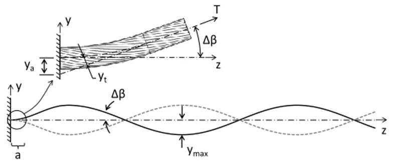
standing wave vibrations (Fig. 1). It also assumes that close to its fixed ends, the conductor deflection departs from the 60
assumed sine shape; the deflection curve asymptotically progresses from a horizontal line (at the clamped end) to a sine-61
shape loop section (Fig. 1). 62 y y ymax Δβ a z yt Δβ T z ya 63
Fig. 1 - Schematization of conductor standing wave vibrations (reproduced from EPRI (2006)) 64
65
Eq. (2.1) defines the strand curvature, while neglecting inertial forces. In this equation, the bending moment (M) results from 66
the multiplication of the axial tension (T) and the departure of the conductor deflection from the sine-shape loop (yt).
67 2 t t 2 d y M T = = y EI EI dz (2.1) 68
For large z values, yt tends to zero. The solution to eq.(2.1) thus becomes yt = Ae-√(T/EI)z, where A is a constant expressed as
69
- T EIz y(z) A =
e - 1+ T EIz[15]. On the other hand, at z = 0 the conductor slope (dyt/dz) is Δβ (Fig. 1). Therefore, assuming
70
small deflection angles, the deflection becomes y(z) = -ya + Δβz + yt [15]. Combining these relations into eq. (2.1) leads after
71
some simplifications to the expression given by eq. (2.2) [15]. 72
0 z A 2 t 2 d y = T EI dz (2.2) 73where y is the conductor deflection amplitude measured at a distance za (Fig. 1). The approach considers independent 74
wires i, and therefore uses a lower bound of the strand bending stiffness (EI) (eq. (2.3)). 75
i=nb wire i 0i i=1 EI = E I (2.3) 76Ei is the Young modulus of the wire i material, and I0i = πdi4/64 for round wires of diameter di. With the conductor curvature
77
defined by eq. (2.2), it is then possible to determine the bending stress level (σa) at the strand fixed end (z = 0).
78 79
4
2.1. Yb method
80
To standardize industry practice, an IEEE committee in 1966 proposed the establishment of a conductor vibration 81
intensity from peak-to-peak deflection (2y), measured at 89 mm (3.5 in) from the clamp exit (Fig. 2). This deflection measure 82
is identified as the Yb parameter.
83 T ±Δβ Yb 89 mm clamp exit 84
Fig. 2 - Standardized conductor dynamic bending amplitude measurement 85
Integrating Yb into eq.2.2 leads to eq. (2.4) also known as the Poffenberger-Swart Formula (PS) [9], where dc is the conductor
86
diameter and z = 89 mm. Eq. (2.4) establishes the alternating bending stress σa. The variable Ea represents the Young
87
modulus of the external layer wire material. 88 c a a - T EIz b T d E 4EI σ = Y e - 1+ T EIz (2.4) 89 2.2. fymax method 90
The bending stress σa may also be evaluated based on the vibration frequency f and the far-field amplitude ymax (Fig. 1),
91
leading to the fymax parameter.
92
At the position where the conductor deflection adopts the sine-shape loop (Fig. 1), the slope dyt/dx corresponds to Δβ, and
93
may be expressed as a fymax function (eq. (2.5)) [4],
94 max 2πfy Δβ = T m (2.5) 95
where m is the conductor mass per unit length. eq. (2.1) may be redefined in terms of fymax , eq. (2.6) [4].
96 2 t max 2 = 0 d y m = 2π fy EI dz z (2.6) 97
σa is then given by eq. (2.7).
98 a c a max m σ = πd E fy EI (2.7) 99
5
2.3. Theoretical endurance limits
100
Based on surveys of numerous experimental conductor fatigue tests, EPRI [4] established endurance limits (at 500 M 101
cycles) for several ACSR in terms of parameters Yb and fymax.
102
For fymax controlled fatigue tests, EPRI suggested endurance limits of 149 mm/s and 118 mm/s for single-layer and
103
multilayer ACSR, respectively. Integrated in eq. (2.7), these limits result in a stress endurance limit σa of 22 MPa for both
104
ACSR types. For fatigue tests performed with imposed Yb values, the EPRI survey defined endurance limits of 0.5 to 1.0 mm
105
for single-layer, and of 0.2 to 0.3 mm for multilayer, ACSR, respectively. Integrated in eq. (2.4), these evaluations lead to 106
stress endurance limits σa of 22.5 MPa and 8.5 MPa for single-layer and multilayer, ACSR, respectively.
107
A comparison of the obtained σa estimates shows that the values are coherent for the single-layer ACSR, whereas for
108
multilayer ACSR, an evident discrepancy appears between the Yb and fymax predictions. This may be attributed to the PS
109
model underlying assumptions which cannot account for wire strand kinematics. 110
In reality, the σa amplitudes derived from this idealized model should only be viewed as an indicator that is well
111
correlated with experimental measurements of conductor fatigue life [16]. Expressing the conductor fatigue performance in 112
terms of parameters Yb and fymax is nevertheless common practice [4]. 113
It is also worth mentioning that these evaluation approaches decouple the endurance limits from the stress causing 114
fretting damages, and therefore, prevent a clear definition of the relationship between wind-induced vibrations and 115
conductor fretting fatigue damages [15]. 116
A refined conductor modeling approach should therefore be useful for obtaining σa estimations which better reflect the
117
physics of the wire strand. 118
119
3. Finite element modeling approach
120
In the following subsection, FE modeling strategy developed in Part I is applied to the ACSR alternating bending stress 121 problem. 122 123 3.1. Model construction 124
The model considers the conductor as rigidly clamped at one end. The other end undergoes fully reversed angular 125
fluctuations of Δβ amplitude under a constant axial tension T (Fig. 3a). 126
6 Modeled portion of length L
T
z y2Δβ
T
y
x
Fixed end cross-sectionb)
a)
127Fig. 3 - FE model configuration (a) and Wire geometric configuration at fixed end (b) 128
129
The model includes a strand section of length L. To facilitate the numerical-analytical σa comparison, the FE models are
130
constructed such that at the fixed end, one of the wire cross-section centers of each strand layer is positioned on the y-axis 131
(Fig. 3b). 132
3.2. Boundary conditions and load configuration
133
The nodes at both end sections are fully coupled with the associated node located at the center core wire. All DOF are 134
constrained at the fixed end, whereas at the free end, only the x displacements and rotations about the z- and y-axes are 135
blocked. The axial load (T) is first applied in the horizontal direction. The Aeolian vibrations are then introduced through 136
reorientations of T at ±Δβ. Angular variations of Δβ are defined in terms of fymax using eq. (2.5). They are gradually induced by 137
increments of 0.1°. Finally, two deflection cycles are simulated in order to achieve a stabilized hysteresis loop (as defined in 138
Part I). 139
3.3 Modeled ACSR
140
The following analysis considers four ACSR strands. The general and stranding properties of the studied conductor are 141
given in Table 1 and Table 2, respectively [17]. In all simulations, the strand length L is fixed at 1000 mm. 142
143
Table 1 - ACSR general properties 144
Properties ACSR 1/0 Drake Crow Bersfort
RTS (kN) 19.5 140.1 117.2 180.1 m (kg/m) 0.216 1.628 1.369 2.370 Ealum. (GPa) 69 69 69 69 Esteel (GPa) 207 207 207 207 EImin (Nm²) 3.9 43.4 18.1 61.6 EImax (Nm²) 24.5 1495 1146 3827 145 146 147 148
7 Table 2 - ACSR stranding properties
149 Layer ni di (mm) E (GPa) αi (⁰) ACSR 1/0 Core 1 3.37 207 - 1 6 3.37 69 6 ACSR Drake Core 1 3.45 207 - 1 6 3.45 207 5.8 2 10 4.44 69 10.7 3 16 4.44 69 12.9 ACSR Crow Core 1 2.92 207 - 1 6 2.92 207 6.34 2 12 2.92 69 10.61 3 18 2.92 69 11.19 4 24 2.92 69 12.49 ACSR Bersfort Core 1 3.32 207 - 1 6 3.32 207 6.2 2 10 4.27 69 9.7 3 16 4.27 69 10.7 4 22 4.27 69 11.7 150
3.4 Inter-wire contact modeling
151
The investigation presented in Part I revealed that while a constant coefficient of friction distribution (μa) offers reliable 152
numerical results, a refined friction model considering the friction coefficient variability and orthotropicity improves the 153
numerical prediction fidelity to experimental measurements. However, in order to minimize the influence of particular 154
modeling adjustments on the results, and also because determining the exact coefficient of friction distributions for ACSR 155
strands submitted to wind-induced loads would be beyond the scope of the present study, the following analysis only 156
considers constant and isotropic friction coefficients. 157
Therefore, μa is set to 0.5 for aluminum-aluminum and aluminum-steel contacts, while a value of 0.3 is applied to
steel-158
steel contacts. 159
160
3.5. Numerical analysis of ACSR strand submitted to bending loads
161
This section presents and analyzes the simulation results obtained for the ACSR listed in Table 1. The study focuses on the 162
conductor deflection and dynamic stress variations predicted close to the clamped region (fixed end). 163
164
3.6. Validation of the modeling approach
165
The following compares the simulation results to the experimental measurements published by Lévesque et al. [18]. In 166
that reference paper, the authors tested three different ACSR types: Drake, Crow and Bersfort. The test bench is described in 167
[19]). The conductors were excited at various controlled modes and ymax amplitudes under axial tension (T) levels
8 corresponding to: 15%, 25% and 35% of the conductor RTS (Rated Tensile Strength). The conductor peak-to-peak deflection 169
amplitudes were measured at multiple locations: at 89 mm from the clamp edge (Yb position), as well as at 45 mm (Yb45), 178 170
mm (Yb178), and 267 mm (Yb267). 171
The experimental configurations were reproduced in the model. Fig. 3a shows the rigid fixed-end conditions integrated in 172
the model to reproduce the square-faced clamp of the experimental system. In addition , in order to obtain precise global 173
trends, the simulations were not limited to the tested fymax, but rather, twenty Δβ values, ranging from 0 to about 2.0°-2.5°, 174
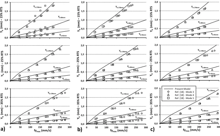
were evaluated for each tension level. Fig. 4 compares the numerical solutions to the Lévesque et al.’s [18] measurements. 175
The comparison graphs include the peak-to-peak deflection amplitudes evaluated at 45 mm (Yb45), 89 mm (Yb89), and 178 mm 176
(Yb178). 177
According to the experimental data shown in Fig. 4, the vibration mode-shape seems to have little influence on the 178
conductor deflection close to the clamp. This observation is in line with the theory presented in Section 2. 179 0,0 0,5 1,0 1,5 2,0 0 50 100 150 200 250 300 Yb (m m ) – 3 5 % R TS fymax(mm/s) 0,0 0,5 1,0 1,5 2,0 Yb (m m ) – 1 5 % R TS 0,0 0,5 1,0 1,5 2,0 Yb (m m ) – 2 5 % R TS 0,0 0,5 1,0 1,5 2,0 0 50 100 150 200 250 300 Yb (m m ) – 3 5 % R TS fymax(mm/s)
b)
Yb 178mm Yb 89mm Yb 45mm Yb 178mm Yb 89mm Yb 45mm Yb 45mm Yb 89mm Yb 178mm 0,0 0,5 1,0 1,5 2,0 Yb (m m ) – 2 5 % R TS 0,0 0,5 1,0 1,5 2,0 Yb (m m ) – 1 5 % RT S 0,0 0,5 1,0 1,5 2,0 0 50 100 150 200 250 300 Yb (m m ) – 3 5 % R TS fymax(mm/s)a)
Yb 178mm Yb 89mm Yb 45mm Yb 178mm Yb 89mm Yb 45mm Yb 45mm Yb 89mm Yb 178mm Present Model Ref. [18] - Mode 3 Ref. [18] - Mode 4 Ref. [18] - Mode 5 0,0 0,5 1,0 1,5 2,0 Yb (m m ) – 2 5 % R TS 0,0 0,5 1,0 1,5 2,0 Yb (m m ) – 1 5 % R TSc)
Yb 178mm Yb 89mm Yb 45mm Yb 178mm Yb 89mm Yb 45mm Yb 45mm Yb 89mm Yb 178mm 180Fig. 4 - fymax vs. Yb for ACSR Drake (a), Crow (b) and Bersfort (c) at T = 15% RTS, 25% RTS and 35% RTS 181
182
The very high correspondence levels displayed in these figures confirm the validity of the proposed modeling approach. 183
Globally, the FE model tends to slightly overestimate the conductor deflection. These differences may result from the 184
assumed friction coefficients. Moreover, despite the apparent linear relationship between fymax and Yb demonstrated by the
9 experimental measurements, the higher resolution obtained with the numerical simulations rather reveal a nonlinear 186
relation between these parameters. 187
188
4. Relation between fymax and Yb criterion
189
As previously mentioned, conductor fatigue performances are commonly defined in terms of fymax or Yb, since both
190
represent measurable parameters. Therefore, depending on laboratory preferences or available equipment, fatigue curves 191
may sometimes be defined with fymax for a certain conductor model, and with Yb for another. This often becomes
192
unmanageable. For example, for a given strand, it might be required to access the bending load severity for known fymax
193
values, while the endurance limit is only defined for Yb. Under such circumstances, EPRI [4] suggests experimentally
194
determining the fymax value that corresponds to the Yb endurance limit. This test should also be performed at the Yb
195
endurance limit amplitude, since, as noted in Section 3, the ratio Yb/fymax does not maintain a stable linear evolution.
196
The proposed modeling procedure offers an attractive alternative to experimental Yb-fymax evaluations. However, the FEA
197
model preparation and computational cost may quickly become prohibitive. It is therefore proposed to establish a Yb
198
predictive tool based on a factorial design approach and built on data generated with the present FE model. 199
The Yb prediction model incorporates the influence of the key factors T, fymax and μa. The role of the adhesive coefficient
200
of friction μa was indeed shown to be significant in Part I. Assuming quadratic variation effects of these parameters, the
201
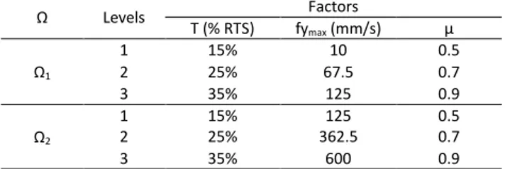
model is built from a three-level (33) factorial design. The selected factor T levels correspond to the usual fatigue data ranges 202
[4]. On the other hand, the μa levels refer to values examined in Part I. For optimal Aeolian vibration coverage, the fymax
203
range goes from 10 to 600 mm/s. Finally, to account for the Yb curvature changes shown in Fig. 4, the fymax interpolation
204
space is further subdivided into two sub-domains (Ω1, Ω2). This subdivision improves the precision of the prediction model. 205
Table 3 presents the factors and the corresponding levels for each Ωi. 206
207
Table 3 - Factors and levels for the interpolation domains (Ω) 208 Ω Levels Factors T (% RTS) fymax (mm/s) μ Ω1 1 15% 10 0.5 2 25% 67.5 0.7 3 35% 125 0.9 Ω2 1 15% 125 0.5 2 25% 362.5 0.7 3 35% 600 0.9 209
All factor combinations presented in Table 3 were simulated with the FE model described in Section 3. Considering each Yb
210
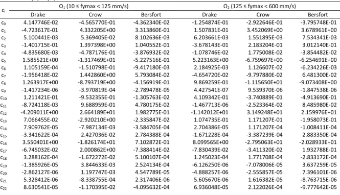
numerical solution as exact, the formulation of the prediction equation can be established based on Lagrange polynomial 211
10 shape functions, leading to eq. (4.1). Table 4 gives the eq. (4.1) coefficients ci for Ω1 and Ω2 including three ACSR: Drake, Crow 212
and Bersfort. Simulations conducted for the single-layer ACSR 1/0, demonstrated that the friction coefficient magnitude has 213
no effect on the conductor deflection (Yb). Fig. 5a presents the model prediction for μa = 0.5 and μa = 0.9. This plot shows that
214
the estimates are perfectly matching. In contrast, Fig. 5b shows the presence of interactions between T and fymax.
215 216 0.0 1.0 2.0 3.0 4.0 0 150 300 450 600 Yb (m m ) fymax(mm/s) T = 15%RTS, μ = 0.5 T = 25%RTS, μ = 0.5 T = 35%RTS, μ = 0.5 T = 15%RTS, μ = 0.9 T = 25%RTS, μ = 0.9 T = 35%RTS, μ = 0.9 0.0 1.0 2.0 3.0 4.0 15% 25% 35% Yb (m m ) T (% RTS) fymax = 10mm/s fymax = 125mm/s fymax = 600mm/s a) b) 217
Fig. 5 – Single-layer ACSR 1/0 Yb variation with (a) fymax and (b) T 218
219
Based on these observations, a two-factor factorial design (32) considering a single fymax interpolation space between 10 and
220
600 mm/s appears to be better adapted. Table 5 presents the factors and the associated levels. The Yb prediction equation
221
reduces to eq. (4.2). Finally, Table 6 gives the ci coefficients.
222
b max
2 2 2 2
0 1 2 max 3 4 max 5 6 max 7 max 8 9 max 10 11 max
2 2 2 2 2 2 2 2 2 2 2 2 2
12 13 max 14 max 15 max 16 17 max 18 max
2 2 19 max 20 max 21 T, fy , = Y c + c T + c fy + c + c Tfy + c T + c fy + c Tfy + c T + c fy + c + c T fy + c T + c T fy + c T fy + c T fy + c T + c T fy + c T fy + c Tfy + c fy + c f 2 2 2 2 2 2 2 2
max 22 max 23 max 24 25 max 26 max
y + c Tfy + c Tfy + c T + c fy + c Tfy
(4.1) 223
Table 4 – Eq. (4.1) ci coefficients 224
ci Ω1 (10 ≤ fymax < 125 mm/s) Ω2 (125 ≤ fymax < 600 mm/s)
Drake Crow Bersfort Drake Crow Bersfort
c0 4.147746E-02 -4.565770E-01 -4.362340E-02 -1.254874E-01 -2.922646E-01 -3.795748E-01
c1 -4.723617E-01 4.332205E+00 3.313860E-01 1.507831E-01 3.452069E+00 3.678961E+00
c2 5.100441E-03 5.369405E-02 8.102636E-03 6.203661E-03 1.551895E-03 7.534341E-03
c3 -1.401715E-01 1.397398E+00 1.040552E-01 -3.678143E-01 2.183204E-01 3.012140E-01
c4 -4.835680E-03 -4.787176E-01 -3.876932E-02 -1.078746E-02 1.775008E-02 -3.854482E-02
c5 1.585521E+00 -1.317469E+01 -5.227516E-01 5.223163E+00 -6.759697E+00 -6.254691E+00
c6 1.105159E-04 -1.510798E-01 -9.417180E-03 2.184925E-03 1.126607E-02 -6.234226E-03
c7 -1.956418E-02 1.442860E+00 5.793084E-02 -4.654720E-02 -9.797880E-02 6.481300E-02
c8 1.263917E+00 -8.793719E+00 -4.156919E-01 9.869259E-01 -1.115650E+01 -9.073408E+00
c9 -1.417234E-06 -3.970819E-04 -2.789478E-05 4.427541E-07 9.539370E-06 -1.847538E-06
c10 1.211421E-01 -9.532355E-01 -1.305763E-02 4.109342E-01 -3.740889E-01 -4.913690E-01
c11 -8.724118E-03 9.688959E-01 4.780175E-02 -1.467713E-06 -2.523364E-02 8.485980E-02
c12 -4.209011E+00 2.664189E+01 1.982775E-01 -1.142012E+01 3.149248E+01 2.159976E+01
c13 7.066455E-02 -2.920210E+00 -2.335847E-02 1.074735E-01 1.171207E-01 -1.958073E-01
c14 7.909762E-05 -7.987134E-03 -3.584705E-04 2.704386E-05 1.171207E-04 -1.008411E-04
c15 -3.341622E-04 2.427036E-02 2.784388E-04 -1.671228E-04 -3.387239E-04 2.883350E-04
c16 3.550401E+00 -1.826174E+01 7.102872E-01 8.099565E+00 -2.795063E+01 -2.028933E+01
c17 -6.745032E-02 2.000862E+00 -7.388414E-02 -7.830439E-02 -3.411320E-02 1.932788E-01
c18 3.288162E-04 -1.672272E-02 5.100107E-04 1.245023E-04 1.771708E-04 -2.833172E-04
c19 -1.385926E-05 3.844633E-03 2.524134E-04 -6.126250E-06 -7.078006E-05 3.637259E-05
c20 -2.862127E-06 1.197747E-03 4.547789E-05 -4.888257E-06 -2.555857E-05 7.396101E-06
c21 5.328412E-06 -8.338755E-04 2.317406E-06 5.605670E-06 1.616382E-05 -8.763715E-06
11
c23 2.153838E-02 -9.861089E-01 1.165334E-02 4.002149E-02 4.845359E-02 -7.321415E-02
c24 -1.355614E+00 9.007796E+00 -1.220868E-01 -4.250385E+00 7.742336E+00 7.448899E+00
c25 -1.187469E-03 1.038677E-01 1.113826E-03 -3.540463E-03 -7.020385E-03 6.325457E-03
c26 -9.738842E-05 8.071674E-03 -8.651218E-05 -5.998786E-05 -1.238360E-04 1.078847E-04
225
Table 5 - Factors and levels for the single-layer ACSR 1/0 case 226 Ω Levels Factors T (% RTS) fymax (mm/s) Ω1 1 15% 10 2 25% 305 3 35% 600 227
Table 6 - Eq. (4.2) ci coefficients for single layer (10 ≤ fymax < 600 mm/s)
228
ACSR 1/0 ci
c0 3.714370E-02 c3 -1.029715E-02 c6 7.059738E-03
c1 -3.401287E-01 c4 6.386957E-01 c7 -4.013036E-06
c2 7.276425E-03 c5 4.069943E-07 c8 9.033446E-06
229
2 2 2 2 2 2b max 0 1 2 max 3 max 4 5 max 6 max 7 max 8 max
Y T, fy
= c +c T +c fy
+c Tfy
+c T +c fy
+c T fy
+c Tfy
+c T fy
(4.2)230
In order to validate the precision of the Yb prediction equation (eqs. (4.1) and (4.2)), Table 7 and Table 8 present a
231
validation plan testing all mid-level factor combinations. 232
Table 7 - Validation plan (single layer ACSR) factor values 233
Mid levels Factors
T (% RTS) fymax (mm/s)
1 20% 157.5
2 30% 452.5
234
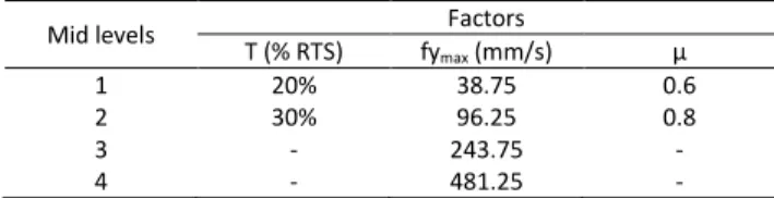
Table 8 - Validation plan (multilayer ACSR) factor values 235
Mid levels Factors
T (% RTS) fymax (mm/s) μ 1 20% 38.75 0.6 2 30% 96.25 0.8 3 - 243.75 - 4 - 481.25 - 236
These combinations were also simulated with the FE model defined in Section 3. Figures 6 and 7 compare the eqs. 4.1 and 237
4.2 Yb prediction values to the FE evaluations. The graphs also include the prediction error bars. 238 239 0.00 0.60 1.20 1.80 20% RTS 243.75 mm/s μ = 0.6 20% RTS 481.25 mm/s μ = 0.6 30% RTS 243.75 mm/s μ = 0.6 30% RTS 481.25 mm/s μ = 0.6 20% RTS 243.75 mm/s μ = 0.8 20% RTS 481.25 mm/s μ = 0.8 30% RTS 243.75 mm/s μ = 0.8 30% RTS 481.25 mm/s μ = 0.8 Yb -FE m o d e l ( m m
) Drake Crow Bersfort
0.00 0.15 0.30 0.45 20% RTS 38.75 mm/s μ = 0.6 20% RTS 96.25 mm/s μ = 0.6 30% RTS 38.75 mm/s μ = 0.6 30% RTS 96.25 mm/s μ = 0.6 20% RTS 38.75 mm/s μ = 0.8 20% RTS 96.25 mm/s μ = 0.8 30% RTS 38.75 mm/s μ = 0.8 30% RTS 96.25 mm/s μ = 0.8 Yb -FE m o d el (m m
) Drake Crow Bersfort
a) b)
240
Fig. 6 - Comparison of Yb values obtained from eq. (4.1) ( (a) Ω1 and (b) Ω2 to FE evaluations with error bars 241
12 0.00 1.00 2.00 3.00 20% RTS 157.5 mm/s 20% RTS 452.5 mm/s 30% RTS 157.5 mm/s 30% RTS 452.5 mm/s Yb -FE m o d e l ( m m ) ACSR 1/0 243
Fig. 7 - Comparison of Yb values obtained from eq. (4.2) (single-layer ACSR 1/0) to FE evaluations with error bars 244
245
Compared to the FE solutions, the prediction equations (eqs. 4.1 and 4.2) demonstrate a high level of correspondence. 246
For example, at T = 20% RTS and fymax = 452.5 mm/s, eq. (4.2) (single-layer ACSR 1/0) leads to practically null deviations; the
247
maximum error is 0.008 mm or 0.33%. On the other hand, compared to the Yb FE solution, the maximum absolute deviation
248
shown by eq. (4.1) (multilayer ACSR) is 0.034 mm (ACSR Bersfort at T = 20% RTS, fymax = 243.75 mm/s and μ = 0.8), while the
249
maximum relative deviation is -7.61% (ACSR Bersfort at T = 20% RTS, fymax = 38.75 mm/s and μ = 0.8).
250
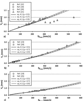
The available conductor endurance limits derived from Yb or fymax were predominantly evaluated for short radius or bell
251
mouth commercial metallic suspension clamps (Fig. 8). On the other hand, the prediction model does not integrate the 252
fixture shape in the simulations. Thus, the precision of the estimation obtained from eqs. 4.1 and 4.2 for practical conditions 253
remains to be evaluated. To that end, Fig. 9 compares the Yb prediction resulting from eq. (4.1) to experimental fymax/Yb
254
measurements extracted from published ACSR fatigue data: Drake [19–22], Crow [23,24] and Bersfort [19,25]. Additionally, 255
to render the friction coefficient effect on Yb estimation more visible, Fig. 9 includes the prediction curves generated when μa
256
= 0.5, 0.7 and 0.9 at the aluminum-aluminum and aluminum-steel contacts. The steel-steel contact coefficient of friction 257 remains fixed at 0.3. 258 LPC T ±Δβ Yb 89 mm Suspension clamp 259
Fig. 8 - Commercial suspension clamp Yb measurement 260
13 0.0 0.5 1.0 1.5 0 100 200 300 400 500 600 Yb (m m ) fymax(mm/s) a) b) c) Ref. [22] Ref. [19] Ref. [20] Ref. [21] eq. 4.1 (μ = 0.5) eq. 4.1 (μ = 0.7) eq. 4.1 (μ = 0.9) 0.0 1.0 2.0 3.0 0 150 300 450 600 750 900 Yb (m m ) fymax(mm/s) Ref. [23] Ref. [24] eq. 4.1 (μ = 0.5) eq. 4.1 (μ = 0.7) eq. 4.1 (μ = 0.9) 0.0 1.0 2.0 3.0 0 100 200 300 400 500 600 Yb (m m ) fymax(mm/s) Ref. [19] Ref. [25] eq. 4.1 (μ = 0.5) eq. 4.1 (μ = 0.7) eq. 4.1 (μ = 0.9) 261
Fig. 9 - Comparison of eq. (4.1) predictions with fatigue measurement of Yb for ACSR at the exit of short radius metallic suspension 262
clamps: (a) Drake, (b) Crow and (c) Bersfort tensioned at T = 25% RTS 263
264
The correlations shown in Fig. 9 are excellent for all three ACSR types. Even in Fig. 9b, where the prediction results from 265
extrapolations outside the limits of the factorial design (fymax > 600 mm/s), the estimations appear to be very close to the
266
measurements. Fig. 9 also reveals that the μa influence remains lower than the scattering of the experimental
267
measurements. Therefore, it is considered that the μa factor may be ignored and eliminated from the factorial design. This
268
simplification results in a unique prediction formulation given by eq. (4.2) for all ACSR types. Moreover, since the Yb
269
estimations made when μa is equal to 0.5 are slightly closer to the experimental measurements, μa is fixed at 0.5 at the
270
aluminum-aluminum and aluminum-steel contacts, while the steel-steel contact coefficient of friction remains unchanged at 271
0.3. Table 9 gives the final eq. (4.2) ci coefficients for the Drake, Crow and Bersfort ACSR.
272
Table 9 - Eq. (4.2) ci coefficients for Drake, Crow and Bersfort ACSR when μa = 0.5 273
ci Ω1 (10 ≤ fymax < 125 mm/s) Ω2 (125 ≤ fymax < 600 mm/s)
Drake Crow Bersfort Drake Crow Bersfort
c0 1.677219E-03 3.813032E-03 5.862408E-03 -2.066610E-01 -2.766266E-01 -3.529718E-01
c1 -1.850450E-02 -3.191341E-03 3.144200E-02 1.699768E+00 2.007805E+00 2.426234E+00
c2 4.858832E-03 4.121085E-03 3.656021E-03 6.411008E-03 5.429836E-03 6.009825E-03
c3 -9.233174E-03 -3.814655E-03 -6.707037E-03 -2.405569E-02 -1.912592E-02 -2.456169E-02
c4 4.701172E-02 -3.820740E-02 -1.194490E-01 -2.698244E+00 -2.397915E+00 -3.376851E+00
c5 -1.516194E-06 -6.677094E-06 -4.490862E-06 -5.999570E-07 8.010386E-07 -3.559112E-07
c6 9.745577E-03 9.006427E-03 1.720596E-02 3.415919E-02 2.479839E-02 3.557543E-02
c7 4.946343E-06 1.057589E-05 2.505030E-05 1.355703E-05 4.362259E-06 1.462084E-05
c8 -5.779415E-06 -3.263413E-05 -8.943414E-05 -2.539196E-05 -7.948543E-06 -2.791612E-05
14 Finally, considering the close agreement shown in Fig. 9 between the prediction and the experimental measurements 275
conjointly with the original numerical model definition, which does not account for the clamping fixture shape, it may be 276
concluded that the short clamp radius has virtually no influence on the bending response evaluated at 89 mm from the Last 277
Point of Contact (LPC). The prediction tool formulated by eq. (4.2) and Tables 7 and 10 may thus be considered as offering 278
reliable evaluations of the bending amplitude of conductors supported by commercial suspension clamps. This simple model 279
provides an instant description of Yb conditions produced by loads defined in terms of T and fymax.
280 281
5. Dynamic bending stress analysis (σa)
282
The FE model developed in Part I can also provide immediate calculations of the alternating stress amplitude (σa), and
283
thus, a direct assessment of the bending load severity via a fatigue damage analysis. 284
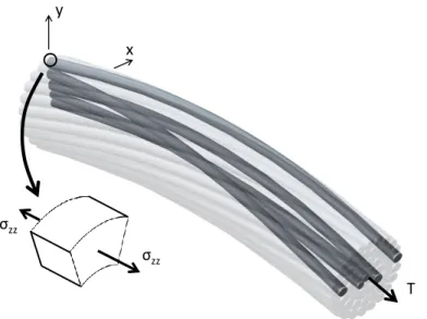
When only considering bulk stresses in configurations similar to that of Fig. 3 submitted to fatigue bending, the most 285
solicited region of each layer appears to be at the extreme fiber of the wires close to the clamped end, and aligned with the 286
y-axis (Fig. 10).
287
The following makes use of the FE model described in Section 3 to determine the σa variations when the four conductors
288
of Table 1 are submitted to fluctuating Yb amplitudes under T = 15%, 25% and 35% RTS. The σa evaluations describe the σzz
289
stress differences (Fig. 10) produced by T between the two-limit angular positions –Δβ and +Δβ. The evaluation is carried out 290
for each aluminum layer. 291
y
x
T
σ
zzσ
zz 292Fig. 10 - Strand orientation for dynamic bending stress (σa) evaluations 293
15 Fig. 11 to present the σa variations calculated for the Yb ranging from 0 to 1 mm. The graphs also include the analytical
295
evaluations produced with eq. (2.4), assuming EImin (eq. 2.3),and EImax. EImax is calculated with eq. (4.3) [26].
296
nb layer i i i i max i i i i c c i A E R cos EI n E I sin
E I
2 3 1 2 (4.3) 297In eq. (4.3), ni, Ai, αi and Ri correspond to the number of wires, the cross-section area, the lay angle, and the layer i radius,
298
respectively. Ec and Ic are the Young modulus and moment of inertia of the core wire. 299
A rapid inspection of the results shows that, on the one hand, the single-layer ACSR results in Fig. 11a demonstrate a 300
perfect match between the FE model and the analytical solution, considering the EImin assumption, which is in agreement
301
with the theory presented in Section 2. On the other hand, the multilayered configurations reveal responses completely 302
different: for all three ACSR (Drake, Crow and Bersfort), at low Yb amplitudes, the σa evaluations follow the EImax assumption,
303
and progressively adopt a trend closer to EImin theory as Yb increases. The stress response evolution systematically begins at
304
lower Yb amplitudes for the outer layer, and progresses toward the inner layers as Yb intensifies. This process corresponds to
305
a progressive interlayer partial deadhesion, which also generates a corresponding load transfer onto the inner layers (causing 306
larger σa). In other words, because of the interlayer sliding, the outer layer wires start bending about their own center fiber
307
instead of respecting a group deformation about the conductor central axis. 308
16 0.0 1.0 2.0 Yb(mm) 0.0 1.0 2.0 Yb(mm) 0 25 50 75 100 125 0.0 1.0 2.0 σa (M Pa ) Yb(mm)
a)
EImax EImax EImax
EImin EImin EImin Layer 1 0 25 50 75 100 125 0.0 0.5 1.0 σa (M Pa ) Yb(mm) 0.0 0.5 1.0 Yb(mm) 0.0 0.5 1.0 Yb(mm)
b)
EImin EImin EImin EImax EImax EImax Layer 2 Layer 3 0.0 0.5 1.0 Yb(mm) 0.0 0.5 1.0 Yb(mm) 0 25 50 75 100 125 0.0 0.5 1.0 σa (M Pa ) Yb(mm)c)
Layer 2 Layer 3 Layer 4 EImin EImax EImin EImax EImin EImax 0 25 50 75 100 125 0.0 0.5 1.0 σa (M Pa ) Yb(mm) 0.0 0.5 1.0 Yb(mm) 0.0 0.5 1.0 Yb(mm) EImin EImax EImin EImax EImin EImaxd)
Layer 2 Layer 3 Layer 4 T = 15% RTS T = 25% RTS T = 35% RTS T = 15% RTS T = 25% RTS T = 35% RTS T = 15% RTS T = 25% RTS T = 35% RTS T = 15% RTS T = 25% RTS T = 35% RTS 310Fig. 11 - Dynamic bending stress - ACSR 1/0 (a), ACSR Drake (b), ACSR Crow (c) and ACSR Bersfort (d) 311
312
For the three analyzed multilayered ACSR, obvious signs of outer layer slip appear around Yb amplitudes between 0.2 and
313
0.5 mm. Actually, a comparison of Fig. 11b) to d) shows that the exact Yb onset level closely depends on the conductor
314
tension (T). Higher axial tensions T engender greater normal forces at the interlayer contact points, and consequently 315
promote the internal conductor friction forces, thus favoring the wire adhesion. 316
317
5.1 Effects of coefficient of friction (μ)
318
Although the results of Section 4.2 revealed a negligible effect of μa on Yb, in view of the last descriptions, the situation
319
may be different for σa. To illustrate the influence of μa on σa, Fig. 12 presents the variation of σa calculated with different μa
320
values for the Drake ACSR over a Yb range of 0 to 2 mm.
17 0 30 60 90 120 150 0.0 0.5 1.0 1.5 2.0 σa (M Pa ) Yb(mm) Δσa (μ = 0.5) Δσa (μ = 0.7) Δσa (μ = 0.9) 0 30 60 90 120 150 0.0 0.5 1.0 1.5 2.0 σa (MPa ) Yb(mm) Δσa (μ = 0.5) Δσa (μ = 0.7) Δσa (μ = 0.9) a) b) EImin EImax EImin EImax 322
Fig. 12 - Variation of σa with Yb in (a) outer layer 3 and (b) inner layer 2 for a Drake ACSR at T = 25% RTS – influence of μa 323
324
As expected, since larger μa values retard inter-wire slippage, and favor a grouped response of the conductor wires, Fig. 12a
325
indicates that σa augments with μa increases. This graph also shows increasing effects of μa on σa with Yb intensifications. Fig.
326
12b displays a similar response for the inner layer. However, because of the larger contributions of the outer layer wires 327
conjointly provoked by μa and Yb, the difference between the prediction curves is of a lesser magnitude. Finally, Fig. 12
328
indicates that the μa influence on the outer layer stress becomes significant for Yb > 0.5 mm. Thus, the friction coefficient
329
effect may be less significant for smaller wind-induced conductor displacements associated with Aeolian vibrations. On the 330
other hand, the coefficient of friction role becomes more significant for galloping transmission lines. 331
332
6. Fatigue life estimation (Nf)
333
Because of the complexity of the problem, current practice usually estimates the conductor fatigue life based on 334
experimental data. In an attempt to establish a universal fatigue criterion for common conductors, the CIGRÉ study 335
committee #22 [27] proposed the σa Safe Border Line eq. (6.1). This semi-empirical expression relates the outer layer
336
alternate bending stress calculated with eq. (2.4) to the number of cycles to failure (Nf). Actually, the safe line described by
337
eq. (6.1) represents a conservative limit established from a collection of experimental measurements that were obtained 338
through standardized fatigue tests involving conductors supported by metallic suspension clamps. 339
-0.20 7 f f a -0.17 7 f f 450 N for N 1.56 ×10 σ = 263 N for N > 1.56 ×10 (6.1) 340The proposed FE model also offers a valuable alternative to estimate Nf. The number of cycles to failure may be
341
calculated from the wire bulk stresses of the outer layer extracted from the numerical simulations for given Yb values, and
18 integrated into any plain fatigue criterion. Obviously, this approach does not explicitly account for the fretting damage 343
contribution. 344
Adopting a basic stress-life approach, the well-known Basquin relation (eq. 6.2) may be selected as the fatigue criterion. 345
Parameters σf’ and b represent the material properties. Table 10 gives these properties for wires made of 1350-H19
346 aluminum [28]. 347
, b a f fσ = σ 2N
(6.2) 348Table 10 - 1350-H19 aluminum properties 349
σy (MPa) σu (MPa) σf’ (MPa) εf’ b c
167 187 204 0.274 -0.07 -0.5
350
The following fatigue life evaluations consider the wire stresses calculated at the critical location of the layers illustrated in 351
Fig. 10. Therefore, they produce fatigue life estimates Nf controlled by the failure of the first wire of the layers.
352
The life predictions generated with the proposed approach are compared below with several published experimental 353
fatigue results extracted from the literature for Drake and Crow ACSR. In all cases, the conductors were tensioned at 25% of 354
their RTS, and supported by fixed short radius metallic suspension clamps. 355
Fig. 13 compares the numerical/experimental fatigue life evaluations obtained for both conductors. To preserve the data 356
presentation form adopted in the references, the graphs display the results with Yb as the damage criterion. They include the
357
FE model-predicted fatigue curves for the two outermost aluminum layers, the experimental data, as well as the Safe Border 358
Line (eq. (6.1)). The reported experimental Nf correspond to cycle numbers at the first wire break. Therefore, for the sake of
359
clarity, the graphs also indicate the wire layer of the first experimental breakage. [29] 360 0.00 0.40 0.80 1.20 1.60 2.00
1.E+04 1.E+05 1.E+06 1.E+07 1.E+08 1.E+09
Yb (mm) Nf 3rdLayer (Ref. [22]) 2ndLayer (Ref. [22]) No break (Ref. [22]) 3rdLayer (Ref. [29]) 2ndLayer (Ref. [29]) 3rdLayer (Ref. [21]) 2ndLayer (Ref. [21])
3rdLayer predicted curve
2ndLayer predicted curve
CIGRÉ Safe border line
a) 0.00 0.75 1.50 2.25 3.00
1.E+03 1.E+04 1.E+05 1.E+06 1.E+07 1.E+08 1.E+09
Yb (m m ) Nf b) 4thLayer (Ref. [23]) 3rdLayer (Ref. [23])
4thLayer predicted curve
3rdLayer predicted curve
CIGRÉ Safe border line
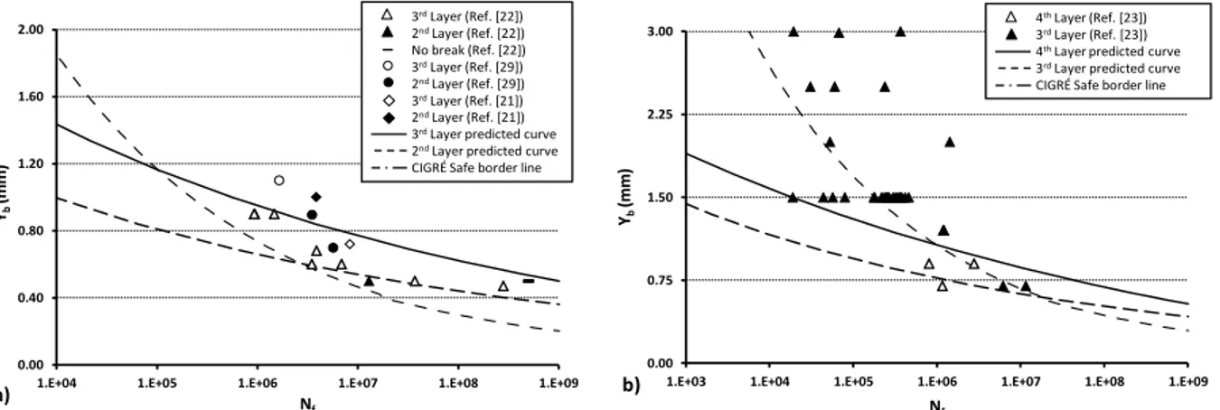
361
Fig. 13 - Yb-Nf 1 st
break for Drake ACSR (a) and Crow ACSR (b) with prediction curves derived from the stress-life eq. (6.2) 362
19 Fig. 13 evidences the scattering present in the experimental data. In fact, this is inherent to stranded conductor experimental 364
investigations, where any slight dimensional, positioning or load variations may significantly affect the local contact 365
conditions. All in all, the eq. (6.2) predicted lives do not wholly reflect the general trends described by the experimental data. 366
Actually, the FE model predictions appear to be in better agreement with the experimental data at low Yb. On the other
367
hand, the CIGRÉ Safe Border Line offers relatively good conductor life estimations. 368
Fig. 11b) and c) show that at Yb values above 0.75 mm, σa becomes very significant, and may presumably cause localized
369
plastic deformations at the different stress risers. Therefore, to improve the model and account for plastic deformation 370
effects, it is proposed to replace the Basquin relation (eq. 6.2) with the also well-known Coffin-Manson fatigue relation (eq. 371
6.3). In this equation, the variable εa is the measured or calculated strain amplitude at the critical location, and εf’ and c are
372
material parameters already introduced in Table 10: 373
,
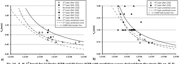
, b c f a f f f σ ε = 2N + ε 2N E (6.3) 374The Fig. 13 fatigue prediction curves were recalculated with eq. (6.3). Fig. 14 compares the new estimates with the 375
experimental measurements and the Safe Border Line results. 376 0.00 0.40 0.80 1.20 1.60 2.00
1.E+04 1.E+05 1.E+06 1.E+07 1.E+08 1.E+09
Yb (m m ) Nf 3rdLayer (Ref. [22]) 2ndLayer (Ref. [22]) No break (Ref. [22]) 3rdLayer (Ref. [29]) 2ndLayer (Ref. [29]) 3rdLayer (Ref. [21]) 2ndLayer (Ref. [21])
3rdLayer predicted curve 2ndLayer predicted curve CIGRÉ Safe border line
a) 0.00 0.75 1.50 2.25 3.00
1.E+03 1.E+04 1.E+05 1.E+06 1.E+07 1.E+08 1.E+09
Yb (mm) Nf b) 4thLayer (Ref. [23]) 3rdLayer (Ref. [23])
4thLayer predicted curve
3rdLayer predicted curve
CIGRÉ Safe border line
377
Fig. 14 - Yb-Nf 1st break for (a) Drake ACSR and (b) Crow ACSR with prediction curves derived from the strain-life eq. (6.3) 378
379
Fig. 14 indicates that the addition of the plastic deformation effect improves the model prediction quality for both the Drake 380
and Crow ACSR. Indeed, now the predicted life curves better correlate with the experimental measurements. In particular, 381
the Crow ACSR graph of Fig. 14b shows that the predictions are now also excellent at very high Yb. This is certainly an
382
indication of the lesser role of the fretting mechanisms in fatigue damage induced under very high Yb. In practice, high Yb
383
amplitudes are usually associated with galloping events. 384
20 The experimental data included also reveal that a majority of the first wire failure occurs at the outer layer for the Drake 385
ACSR, while it is the opposite for the Crow ACSR, where the wires of the inner layer seem to be the most susceptible to 386
fracture. This is presumably due to the lower Yb of the fatigue test conditions maintained for the Drake ACSR, as compared to
387
the Crow ACSR. Indeed, greater deflection amplitudes favor the slippage of the outermost wire, and thus reduce the load 388
they support. The layers underneath consequently sustain higher stress levels, resulting in more rapid fatigue crack growth. 389
On the other hand, at low Yb, the wires of the outer layer share a larger part of the total load and are more severely affected
390
by the fatigue crack propagation than the inner layers. 391
Fig. 14 also shows that in all cases, the FE model predicts a first wire break in the inner layer, which is not in perfect 392
agreement with the experimental measurements. On the other hand, it is consistent with the numerical results of Fig. 11b) 393
and c). This difference with the experimental measurements may be explained in part by underestimated friction coefficients 394
(μa), especially in the clamped region. Indeed, Fig. 12 shows that higher μa tend to increase the outer layer stress, while 395
having less of an effect on the inner ones. The boundary conditions considered in the FE model in lieu of the real shape of the 396
clamping fixture may also affect the outer layer slippage conditions. 397
In addition, the wear damages occurring at inter-wire contact points, which are not explicitly considered within the 398
present fatigue formulation (eq.6), also certainly contribute to the differences between the experimental and numerical life 399
predictions. The prevailing inter-wire contact regime may generate either sticking, gross slip or mixed conditions. While the 400
sticking condition considerably reduces wear phenomena, gross slips lead to important wear rates. Therefore, since wear and 401
fatigue are competing degradation modes, as supported by experimental measurements the mixed conditions associated 402
with lower wear rates and rougher surfaces appears as the most detrimental regime [30]. Therefore, investigations focusing 403
on the identification and the adaptation of a damage criterion better accounting for contact conditions, such as those 404
published in Ref. [32,33], or considering wear laws as in Ref. [14], may contribute to refined the conductor life prediction 405
obtained from the present FE model. 406
Finally, while the developed FE model precision may further be improved (with the addition of the suspension clamps and 407
the incorporation of a refined damage criterion accounting for fatigue-wear interactions), the prediction accuracy remains 408
quite high overall. The numerical results in Fig. 14 compare well with the experimental measurements, as well as with the 409
semi-empirical estimations resulting from the CIGRÉ formula (eq. 6.1). Actually, because the omission of the clamp in the 410
model reduces the calculation times considerably, the modeling strategy presented represents an effective trade-off. 411
21
7. Conclusion
412
The present paper made use of the FE modeling strategy developed in Part I to study the internal strain-stress conditions 413
of ACSR conductors submitted to wind-induced loads. The first portion of the investigation examined the descriptors Yb and
414
fymax used by researchers and industrial designers to evaluate load severity. The tests directly underlined the discrepancies
415
between these descriptors, along with the difficulty in coupling them in conductor life prediction. The main objective of the 416
second portion of the analysis was to evaluate an alternative way of investigating the conductor fatigue problem based on 417
realistic stress/strain descriptions. 418
The study included four ACSR covering single- to four-layer configurations. Initial comparisons with reference 419
experimental test data demonstrated the ability of the FE model to predict the bending deflection amplitudes Yb in the near
420
field of the clamped zone from the far-field vibration parameter fymax.
421
In order to circumvent the incompatibility existing between Yb and fymax, and to provide a practical strategy for accurately
422
relating them, a numerical evaluation of their responses integrated into a factorial design approach led to a multivariate 423
prediction equation for Yb. The resulting model provides instantaneous predictions of Yb as a function of selected fymax, T and
424
μa values within an error level less than 8% when compared to a full 3D FE analysis. Additional comparisons of the predicted
425
Yb with reference experimental measurements also demonstrated the applicability of the equation to conductors supported
426
by commercial metallic suspension clamps. This simple model offers an easy way of converting and relating reference data 427
established by various laboratories following specific standards and different research goals. 428
Because the practical descriptions of Yb and fymax cannot depict the relationship connecting the experimental endurance
429
limit and the strain-stress conditions causing fatigue damages, the study examined the merits of life predictions made from 430
basic stress/strain damage analysis. Disregarding the effect of contact stresses, the investigation only considered the bulk 431
stress/strain amplitudes of the wire to estimate the conductor residual life. Comparisons with experimental data of two 432
multilayered ACSR indicated that the fatigue prediction curves established from the Coffin-Manson fatigue relation provides 433
realistic evaluations of the service life of conductors submitted to both low amplitude deflections generated by wind-induced 434
vibrations and high amplitude deflections resulting from line galloping. 435
436 437 438
22
Acknowledgments
439
This research project was funded by the Natural Sciences and Engineering Research Council (NSERC) of Canada and the 440
Hydro-Quebec/RTE - Structure and mechanics of power transmission lines research chair at Sherbrooke University. 441
442
References
443
[1] Irvine M. Local bending stresses in cables. Int J Offshore Polar Eng 1993;3:172–5.
444
[2] Raoof M, Davies TJ. End fixity to spiral strands undergoing cyclic bending. J Strain Anal Eng Des 2005;40:129–37.
445
[3] Zhou ZR, Cardou A, Goudreau S, Fiset M. Fundamental investigations of electrical conductor fretting fatigue. Tribol Int
446
1996;29:221–32. doi:10.1016/0301-679X(95)00074-E.
447
[4] EPRI. EPRI Transmission line reference book: Wind-induced conductor motion. Palo Alto, CA: 2006.
448
[5] Cardou A, Jolicoeur C. Mechanical models of helical strands. Appl Mech Rev 1997;50:1–14.
449
[6] Lalonde S, Guilbault R, Légeron F. Modeling multilayered wire strands, a strategy based on 3D finite element beam-to-beam
450
contacts - Part I: Model formulation and validation. TBD 2016;TBD:TBD.
451
[7] Ouaki B, Goudreau S, Cardou A, Fiset M. Fretting fatigue analysis of aluminium conductor wires near the suspension clamp:
452
Metallurgical and fracture mechanics analysis. J Strain Anal Eng Des 2003;38:133–47.
453
[8] B2.30 CW group. Engineering guidelines relating to fatigue endurance capability of conductor/clamp systems. Cigre Tech Broch No
454
429 2010:42 p. – 42 p.
455
[9] Poffenberger JC, Swart RL. Differential displacement and dynamic conductor strain. IEEE Trans Power Appar Syst
1965;PAS-456
84:508–13.
457
[10] B2.11.07 CT force. Fatigue endurance capability of conductor / clamp systems: update of present knowledge. Cigre Tech Broch No
458
332 2007:63 p. – 63 p.
459
[11] Cardou A. Taut helical strand bending stiffness. UFTscience 2006.
460
[12] Giglio M, Manes A. Life prediction of a wire rope subjected to axial and bending loads. Eng Fail Anal 2005;12:549–68.
461
doi:10.1016/j.engfailanal.2004.09.002.
462
[13] Costello GA. Theory of wire rope. 2\superscr ed. New York: Springer-Verlag; 1990.
463
[14] Argatov II, Gómez X, Tato W, Urchegui MA. Wear evolution in a stranded rope under cyclic bending: Implications to fatigue life
464
estimation. Wear 2011;271:2857–67. doi:10.1016/j.wear.2011.05.045.
465
[15] Goudreau S, Levesque F, Cardou A, Cloutier L. Strain Measurements on ACSR Conductors During Fatigue Tests II—Stress Fatigue
466
Indicators. IEEE Trans Power Deliv 2010;25:2997–3006. doi:10.1109/TPWRD.2010.2042083.
467
[16] Cloutier L. Technology watch for gaps in knowledge about conductor fatigue - T083700-3355. Bromont: 2009.
468
[17] Langlois S, Legeron F, Levesque F. Time History Modeling of Vibrations on Overhead Conductors With Variable Bending Stiffness.
469
IEEE Trans Power Deliv 2013.
470
[18] Levesque F, Goudreau S, Langlois S, Legeron F. Experimental Study of Dynamic Bending Stiffness of ACSR Overhead Conductors.
471
IEEE Trans Power Deliv 2015;30:2252–9. doi:10.1109/TPWRD.2015.2424291.
472
[19] Levesque F, Goudreau S, Cardou A, Cloutier L. Strain Measurements on ACSR Conductors During Fatigue Tests I—Experimental
473
Method and Data. IEEE Trans Power Deliv 2010;25:2825–34. doi:10.1109/TPWRD.2010.2060370.
474
[20] Brunair RM, Ramey GE, Duncan RR. An experimental evaluation of S-N curves and validity of Miner’s cumulative damage
475
hypothesis for an ACSR conductor. IEEE Trans Power Deliv 1988;3:1131–40. doi:10.1109/61.193895.
476
[21] Dalpé C. Interaction mecanique entre conducteur electrique aerien et pince de suspension: Etude sur la fatigue, la rigidite et la fip.
477
Laval University, 1999.
478
[22] Levesque F, Goudreau S, Cloutier L, Cardou A. Essais en fatigue sur le conducteur ACSR Drake - Rapport No. SM-2006-01. Quebec:
479
2006.
23
[23] Jolicoeur C, Goudreau S, Cardou A, Cloutier L. Essais de fatigue d’un conducteur crow avec différentes pinces de suspension sous
481
fortes amplitudes de vibration simulant les conditions de galop - Rapport No. SM-2005-04. Quebec: 2005.
482
[24] Luc S. Cumul d’endommagement par fatigue d'un conducteur ACSR. Sherbrooke University, 2006.
483
[25] Levesque F. Etude de l’applicabilite de la regle de Palmgren-Miner aux conducteurs electriques sous chargements de flexion
484
cyclique par blocs. Laval University, 2005.
485
[26] Cardou A. Stick-slip mechanical models for overhead electrical conductors in bending (with Matlab® applications). Quebec: 2013.
486
[27] CIGRE Study Committee #22. Endurance capability of conductors. 1988.
487
[28] Lévesque F, Légeron F. Contact mechanics based fatigue indicator for overhead conductors 2010.
488
[29] Jolicoeur C, Goudreau S, Cardou A, Cloutier L. Essais en fatigue sur les conducteurs Bersfort et Drake - Rapport No. SM-2001-03.
489
Quebec: 2000.
490
[30] Zhou ZR, Vincent L. Mixed fretting regime. Wear 1995;181-183:531–6.
491
[31] Zhou ZR, Cardou A, Fiset M, Goudreau S. Fretting fatigue in electrical transmission lines. Wear 1994;173:179–88.
492
[32] Szolwinski MP, Farris TN. Mechanics of fretting fatigue crack formation. Wear 1996;198:93–107.
493
[33] Alfredsson B, Cadario A. A study on fretting friction evolution and fretting fatigue crack initiation for a spherical contact. Int J
494
Fatigue 2004;26:1037–52.
495 496