Actuator / Sensor Placement and Experimental Modal Analysis on
Piezo-Structures
Pascal De Boe (1), Jean-Claude Golinval (2)
Université de Liège, LTAS – Vibrations et Identification des Structures, 1, Chemin des chevreuils, B52, B-4000 Liege (Belgium)
(1)
[email protected], (2) [email protected], http://ulg.ac.be/ltas
1 Abstract
Few works have been performed in the field of experimental modal analysis by means of piezoelectric distributed elements. Piezoelectric laminates, initially intended for the monitoring and the control of smart structures, could also be dedicated to the experimental modal identification of an open-loop structure. A pole-residue development of the open-loop piezo-structure shows that conventional algorithms and a piezoelectric pseudo-collocated actuator/sensor may be used to estimate the mechanical modal parameters.
When an initial mathematical model of the structure is available, the 'best' excitation position is determined by checking the H2 norm of the transfer
function of the fully observed system. The same methodology can be applied for the selection of the monitoring locations. In most cases, experimental testing with the selected sensors set, gives acceptable information to identify target modes. These data, coupled with electrical sensing at the piezoelectric element level, can then be used to perform the modal analysis of the piezo-structure.
A light clamped-free plate instrumented with piezo-laminates is used to illustrate this experimental approach.
2 The dynamic analysis of
piezo-structures
2.1 Modal analysis of a conventional structure
The resolution of the eigenvalues problem of a conventional linear structure :
( 1 ) M ⋅x+D ⋅x+K ⋅x =f
yields to n pairs of complex conjugate eigenvalues :
( 2 ) pi i,+n = − ⋅ζi ωi ± ⋅j ωi ⋅ 1−ζi i =1 2, , n
2 …
associated with n complex eigenvectors
[
]
Φ = φ1 φ2 … φn , where ωi is the i
th
natural frequency of the conservative structure and ζi is the
corresponding damping coefficient (see Géradin and Rixen [4]). For a force fl applied at the spatial position l and for a response xk measured at the
spatial position k, the frequency response function (FRF) is expressed by : ( 3 ) ( )
[
]
[
]
α ω φ φ ω φ φ ω kl ki li i i ki li i i i n m j p m j p = ⋅ ⋅ ⋅ − + ⋅ ⋅ ⋅ − ⎧ ⎨ ⎪ ⎩⎪ ⎫ ⎬ ⎪ ⎭⎪ = ∑ * * * 1where mi is the modal mass associated with the i
th
mode φi.
2.2 Modal analysis of a piezo-structure
In the case of a structure instrumented with a piezoelectric sensor/actuator, electromechanical relationships are added to the previous system ( 1 ) to represent contributions of the electrical degrees of freedom linked to the piezoelectric actuator and sensor (Saunders et al. [3]) :
( 4 ) M x D x K x f v x C v q a a s p s T ⋅ + ⋅ + ⋅ = + ⋅ ⋅ + ⋅ = Θ Θ
The first equation is commonly called the actuator equation and the second, the sensor equation. The actuator equation exhibits the force generated by the piezoelectric actuator through the electromechanical coupling actuator matrix Θa
and the electrical potential va applied between the electrodes of the
element. On the other hand, the sensor equation shows the relationship existing between the mechanical degrees of freedom x and the electrical charges q or potentials vs through the
electromechanical coupling matrix ΘsT
and the capacitance Cp of sensor.
In the case of a force applied on a structure instrumented by a piezoelectric sensor, and by forcing the electrode potentials to zero with a short-circuit (e.g. : physically, by means of a perfect charge amplifier), we can write :
( 5 ) M x D x K x f x q sT ⋅ + ⋅ + ⋅ = ⋅ = Θ
From ( 3 ), it can be found that :
( 6 )
[
]
[
]
v f m j p m j p s l s i li i i s i li i i i n T T = ⋅ ⋅ ⋅ ⋅ − + ⋅ ⋅ ⋅ ⋅ − ⎧ ⎨ ⎪ ⎩⎪ ⎫ ⎬ ⎪ ⎭⎪ = ∑ Θ φω φ Θ φ φ ω * * * 1This equation is very important because it states that the determination of the electromechanical coupling
matrix Θs is theoretically possible by means of an
experimental modal analysis and an adequate set of measurements. Extraction of the modes, eigen-frequencies, modal damping and modal masses could be performed with conventional modal analysis algorithms applied on experimental structural F R F s. Note that correct estimation of modes needs measurement at a driving point, i.e. where excitation and response are measured at the same position and in the same direction (see Ewins [1] and Maia, Silva et al. [2]).
2.3 Structural modal analysis using piezoelectric distributed transducers
Let us consider the case where no direct mechanical force is applied on the system but only consider the effect of a piezoelectric actuator. Comparing ( 1 ) to ( 4 ), it is easy to understand the substitution of fl for Θa a v ⋅ in ( 3 ) : ( 7 ) ( )
(
)
x m j p m j p v i i T a i i i i T a i i i n a = ⋅ ⋅ ⋅ ⋅ − + ⋅ ⋅ ⋅ ⋅ − ⎡ ⎣ ⎢ ⎢ ⎤ ⎦ ⎥ ⎥⋅ = ∑ Φ Φω Θ Φ* * Φω Θ * * 1which links the structural displacements to a voltage applied to the piezoelectric actuator. It is clear that the poles of this system are identical to ( 1 ). Nevertheless, in the case of a modal analysis, the residue estimation is not direct. One way to overcome this problem is to use costly technologies as a sensori-actuator or, more easily, a pseudo-collocated actuator / sensor. This last technique is very well adapted in the case of plate-type structures by simply fixing piezo-laminates on each sides of the tested plate.
3 Excitation and measurement point
selection for experimental modal analysis
The selection of the optimal positions of excitation and sensing is not a simple task. Without any criteria, engineer judgement and various trials are needed to obtain an acceptable set of data in order to perform a correct identification of modes in the frequency range of interest. This procedure is time-consuming and not very effective. The problem of actuator and sensor placement have been already investigated in literature. Kammer [5] proposes the selection of the best signal to noise ratio position. In Gawronski [6], the procedure is based on the monitoring of the observability and controllability Grammians to choose optimal excitation and sensor locations. This paper addresses the problem of
punctual actuator and sensor placements; location
strategies for distributed actuators and sensors will be presented in the near future.
3.1 State-space modal representation
To apply the theory of controllability and observability, which has been developed in the theory of control, it is convenient to express the
generalised (multi-excitations and outputs) system nodal representation ( 1 ) in the form :
( 8 ) M x D x K x B f y C x x C x x ⋅ + ⋅ + ⋅ = ⋅ = ⋅ + ⋅ 0 0 0
where y is defined as the output vector and depends linearly of the structural displacements and velocity. Defining the state variables as the modal displacement and velocities :
( 9 ) X x x m m m =⎧⎨⎪ ⎩⎪ ⎫ ⎬ ⎪ ⎭⎪
the modal state-space form :
( 10 ) X A X B f y C X m m m = ⋅ + ⋅ = ⋅
is defined by the following triplet :
( 11 ) A
[
]
I Z B Bm C C C mx mx = − − ⎡ ⎣ ⎢ ⎢ ⎤ ⎦ ⎥ ⎥ = ⎡ ⎣ ⎢ ⎢ ⎤ ⎦ ⎥ ⎥ = 0 2 0 2 Ω . .Ω, ,where Ω = diag(ω ω1, 2,…ωn) is the spectral matrix
associated with the (n ×nm) modal matrix
[
]
Φ = φ1 φ2 … φnm . The modal mass, damping
(assuming proportional damping for convenience) and stiffness diagonalized matrix are obtained by the modal projection on K , D , M : ( 12 ) M M D D K K Z M D m T m T m T m m = = = = − − Φ Φ Φ Φ Φ Φ Ω . . , . . . . , 1. . . 2 1 1
In the same way, the modal input, displacement and velocity output matrices are introduced by :
( 13 ) Bm Mm B C C C C T mx x mx x = −1 = = 0 0 0 .Φ . , .Φ, .Φ
3.2 Controllability and observability
In classical control theory (see Kwakernaak and Sivan [7]), controllability and observability matrices are checked. As clearly explained in Gawronski [6], these criteria, although simple, are not at all efficient :
• the level of controllability or observability is not quantified; but these criteria give an answer in term of yes or no.
• The computation of these matrices is prohibitive in case of system with realistic size.
These two drawbacks bring us to prefer expressing the system properties in term of Grammians. The controllability and observability Grammians are defined as follows : ( 14 ) ( ) ( ) W t e B B e dt W t e C C e dt c A t T t A t o A t T t A t T T = ⋅ ⋅ ⋅ = ⋅ ⋅ ⋅ ⋅ ⋅ ⋅ ⋅ ∫ ∫ 0 0
The controllability Grammian reflects the ability of a perturbation f to perturb the state of the system. The observality Grammian reflects the ability of a state X to affect the output y of a system. In the
case of a time invariant system, the stationary solutions of ( 14 ) are given by the Lyapunov equations : ( 15 ) A W W A B B A W W A C C c c T T T o o T ⋅ + ⋅ + ⋅ = ⋅ + ⋅ + ⋅ = 0 0
3.3 Transfer function norm and placement strategy
The transfer function of a system, expressed in the state-space form, is given by :
( 16 ) G( )ω =C ⋅(j ⋅ω⋅I −A)−1⋅B
For flexible systems in the modal state representation, theH2 norm can be expressed in
terms of the norms of the modes. This modal decomposition affords then a visibility on each modal contributions. The transfer function of the ith mode is expressed by :
( 17 ) Gi( )ω =Cmi ⋅(j⋅ω⋅I −Ami)−1⋅Bmi
By ( 17 ) and since the Grammians are diagonally dominant in the modal state-space representation, the H2 norm of the complete system is estimated by
the rms sum of the modal norms :
( 18 ) G Gi i nm 2 2 2 1 ≅ = ∑
Equation ( 18 ) is the base for actuator and sensor placement strategy.
The procedure starts with the selection of the best actuator position. Assuming that all degrees of freedom are monitored, we compute the placement index σ2ki that evaluates the importance of the k
th
actuator at the ith mode on the global transfer function H2 norm : ( 19 ) σ2 2 2 ki ki ki w G G = ⋅
which clearly shows the ability of the kth actuator position to affect the ith mode. Once the actuator positions are selected (B0 optimised), the same
procedure can be repeated by constructing a sensor placement indice matrix, helping the selection of the best sensor positions.
4 Experimental
set-up
A 0.16 x 0.08 x 0.001 m clamped-free stainless steel plate, fitted with one commercial piezoelectric laminate on each face will be studied to illustrate the method. These two 0.0508 x 0.0254 x 0.0004 m piezoelectric (PZT) laminates are placed in a pseudo-collocated configuration, near the clamped side of the plate (see figure 1).
Figure 1 : Experimental set-up
4.1 Finite element model
In order to determine the optimal locations of sensors and actuator (e.g. : an impact hammer), the tested structure was first modelled with the finite element (F.E.) technique.
The first five computed modes of the tested structure are presented in figure 2 (note the meshing and the thickness / length ratio).
(a) (b) (c) (d) (e) (a) 27.9 hz (b) 134.3 hz (c) 165.8 hz (d) 442.7 hz (e) 473.2 hz
Figure 2 : Finite element modes
4.2 Optimal actuator and sensor location
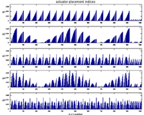
Once a model is available and modes targeted, the procedure described in §3.3 is used to find the more efficient position to impact the structure. Figure 3 shows a graphical representation of the actuator placement indices for the 5 first modes.
As expected, controllability of actuator position is best at the two corners, located at the opposite of the clamping side. Direction of excitation is of course perpendicular to the plate.
Once the excitation point is selected, the sensor placement indice matrix is also constructed for the selection of the best sensor positions. As for the excitation selection, the best sensor positions are given at the plate corner.
4.3 Impact hammer test
Due to the light weight of the structure, non-contact measurement technique, by means of a LASER vibrometer, has been preferred. Figure 4 shows the comparison between the identified experimental modes (from a circle fitting algorithm) and the F.E. modes by means of the extensively used
Modal Assurance Criterion (MAC) which is defined
as follows : ( 20 )
(
)
(
)
M A C ( X i A j X i T A j X i T X i A j T A j φ φ φ φ φ φ φ φ , ) = ⋅ ⋅ ⋅ ⋅ 2where subscript X is applied for experimental mode
and subscript A is applied for modes extracted from
a model. The M A C always lies between 0 (no correlation between modes) and 1 (modes are perfectly correlated). 1/27.9 2/134.2 3/165.7 4/442.7 5/473.1 1/24.2 2/118.7 3/148.2 4/376.2 5/408 FE Im pa c t h am m er ac tu at or 0 0.1 0.2 0.3 0.4 0.5 0.6 0.7 0.8 0.9 1
Figure 4 : FE / hammer MAC
Results show a very good correlation except for the last mode.
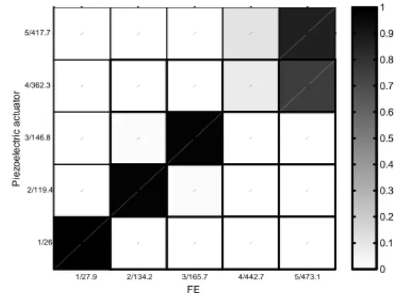
4.4 Piezolaminate actuator test
The technique, presented in §2.3 has been tested on the same structure. A burst-chirp signal [ 5 - 500 hz ] was applied to the upper piezolaminate element. Figure 5 presents the obtained M A C : except for mode 4, all the modes have a very good correlation. 1/27.9 2/134.2 3/165.7 4/442.7 5/473.1 1/26.4 2/119.4 3/146.8 4/362.3 5/417.7 FE P iez oel ec tr ic ac tu at or 0 0.1 0.2 0.3 0.4 0.5 0.6 0.7 0.8 0.9 1
Figure 5 : FE / piezolaminate MAC
5. Conclusion
This paper has demonstrated the feasibility of the experimental modal identification by means of integrated piezoelectric laminates. Results are improved by using tools to find the optimal location of distributed piezoelectric elements.
Acknowledgements
This work has been financed by the Région
Wallonne of Belgium under the contract RW-ULG 9613500.
Bibliography
1. Ewins, D.J., Modal testing : theory and practice, Research Studies Press LTD., England, 1984. 2. Maia, Silva , He, Lin, Skingle, To, Urgueira,
Theoretical and experimental modal analysis,
Research Studies Press LTD., Taunton, England, 1997.
3. Saunders, W.R., Cole, D.G., Robertshaw, H.H., Experiments in piezostructure modal analysis for MIMO feedback control, Smart Mater. Struct., 1994, 3, 210-218.
4. Géradin, M., Rixen, D., Mechanical vibrations,
Theory and application to structural dynamics,
Wiley, Chichester, England, 1993.
5. Kammer, D.C., Sensor placement for on-orbit modal identification and correlation of large space structures, Journal of Guidance Control and
Dynamics, 14, 251-259.
6. Gawronski, W.K., Dynamics and control of structures : a modal approach, Springer-Verlag,
New-York, 1998
7. Kwakernaak, H.K., Sivan, R., Linear optimal