Virtual Insanity: Linear Subnet Discovery
Jean-François Grailet, Benoit Donnet
Université de Liège, Montefiore Institute, Belgium
Abstract—Over the past two decades, the research community has developed many approaches to study the Internet topology. In particular, starting from 2007, various tools explored the inference of subnets, i.e., sets of devices located on the same connection medium which can communicate directly with each other at the link layer.
In this paper, we first discuss how today’s traffic engineering policies increase the difficulty of subnet inference. We carefully characterize typical difficulties and quantify them in the wild. Next, we introduce WISE (Wide and lInear Subnet inferencE), a new tool which tackles those difficulties and discovers, in a linear time, large networks subnets. Based on two ground truth networks, we demonstrate that WISE outperforms state-of-the-art tools. Then, through large-scale measurements, we show that the selection of a vantage point with WISE has a marginal effect regarding accuracy. Finally, we discuss how subnets can be used to infer neighborhoods (i.e., aggregates of subnets located at most one hop from each other). We discuss how these neighborhoods can lead to bipartite models of the Internet and present validation results and an evaluation of neighborhoods in the wild, using WISE. Both our code and data are freely available.
Index Terms—WISE, subnet, flickering, warping, neighborhood
I. INTRODUCTION
For now nearly two decades, the Internet topology has been investigated at multiple levels [1]. The most basic point of view is the IP interface level where data is revealed through hop-by-hop exploration performed by traceroute and its variants (e.g., Paris traceroute [2]). Second, multiple interfaces of a given router might be aggregated into a single identifier through alias resolution, leading to a router level view of the Internet topology. Finally, the higher level would be the Autonomous System (AS) level modeling relationships between ASes and is captured, for instance, through BGP routing information.
Besides this academic view of the Internet topology, ad-ditional intermediate levels have emerged over time. For instance, Internet eXchange Points (IXPs) [3], [4] or Points-of-Presence (PoPs) [5], [6] are more and more investigated. This paper is in the scope of an another intermediate level:
sub-networks(or, more simply, subnets), i.e., a set of devices
that are located on the same connection medium and that can communicate directly with each other at the link layer [7]. Exploring subnets is a way to enrich router level maps by providing particular topological features of ISP networks. Subnet inference has been studied as soon as 2007 [8], with the introduction of an inference technique based on IP address assignment practices.
State-of-the-art techniques for revealing subnets are based on active probing and on-the-fly complex rules for building each subnet [9], [10], [11]. However, those tools, usually
involving a single machine (or vantage point) to perform the probing work, fail to reveal accurate subnets in the presence of traffic engineering policies, such as load-balancing [12], [13], applied by domains.
In this paper, we first review the most common phenomena that increase the difficulty of subnet inference for such tools and elaborate on what kind of traffic engineering policies could cause them. Then, we introduce a novel tool, WISE (Wide and lInear Subnet inferencE), that is designed to detect these phenomena and take them into account while discovering subnets. WISE not only carefully evaluates the IP addresses considered for subnet inference, but also achieves it without additional probing and in linear time (i.e., the execution time will be proportional to the amount of involved IP interfaces). Indeed, WISE is built to first collect the data it needs for subnet inference, while previous state-of-the-art tools [9], [10], [11] usually discovers subnets while probing.
This paper provides four contributions.
1) we characterize and evaluate modern subnet inference challenges (Sec. II);
2) we introduce a new tool (WISE) that can work around these issues while performing better than state-of-the-art subnet inference tools [10], [11] (Sec. III). We validate
WISEwith respect to state-of-the-art tools based on two
ground truths (Sec. IV);
3) by analyzing data collected with WISE from the PlanetLab testbed, we evaluate the effects of changing the vantage point from one measurement to another, as encountered traffic engineering issues will likely change as well (Sec. V). Through this, we demonstrate that WISE can usually discover similar sets of subnets despite vantage point change.
4) finally, we expand on our previous work [14] by dis-cussing how subnets can be used as a first step towards a comprehensive discovery of a target domain. We present the concept of neighborhood (i.e., a location bordered by subnets located at most one hop from each other) and introduce the notion of peer, used to locate neighborhoods with respect to each other. Then, we discuss how a neighborhood-based graph can lead to bipartite models of networks [15]. We elaborate on these concepts by discussing how we modified WISE to discover neighborhoods and their peers, by validating them on our ground truth networks and by evaluating their viability in the wild, using network snapshots collected from PlanetLab nodes in Fall 2019.
WISEsource code, our figures, and the scripts for generating
them (or scheduling a campaign) are all available online.1
II. SUBNETINFERENCECHALLENGES A. State-of-the-Art inference
A subnetwork, or subnet, consists in a set of devices, each of them being identified by a unique IP address, that are all connected together through the same connection medium. In the Internet, a subnet can be a point-to-point link as well as a local area network (LAN) isolated in the network topology. From the perspective of a single vantage point, and in the (near) absence of traffic engineering policies, interfaces of a same subnet will appear as a set of IP addresses that are consecutive with respect to the IP scope and that are located at the same distance. This distance is typically estimated by a Time-To-Live (or TTL) value which is the minimal TTL value the vantage point can use in a probe packet to get a reply from the targeted subnet interface. Interfaces are also typically reached through a similar route in the network, i.e., the last interface(s) appearing in the routes towards distinct subnet interfaces should be identical.
Ideally, a subnet should also contain at least one interface that belongs to the last router crossed before entering the subnet, and that therefore appears one hop closer to the measurement vantage point than other subnet interfaces. In
TraceNET[9] and ExploreNET [10] terminology (as well
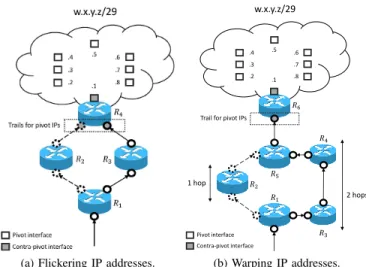
as TreeNET [11]), interfaces belonging to the subnet that are not located on the last crossed router are called pivot interfaces while the interface(s) located on this router are called contra-pivot interfaces, as illustrated in Fig. 1 (pivots are white squares, while contra-pivots are depicted by gray squares). It should be noted that, while having a single contra-pivot interface makes more sense at first glance, it is actually possible to find more than one contra-pivot because routers may implement back-up interfaces to reach critical subnets. In practice, we have observed such a scenario in the academic ground truth we used for our validation (see Sec. IV).
All state-of-the-art tools take advantage of those ideas to reveal subnets. TraceNET uses traceroute-like probing towards a set of target IP addresses and, then, analyzes the collected routes to identify the subnets crossed to reach the destinations. ExploreNET probes a growing range of IP addresses consecutively (starting with a single initial target, then building a /31 or /30, then a /29, etc.) to build a subnet that keeps expanding as long as a few rules are fulfilled and as long as responsive interfaces can be found. Finally, TreeNET builds itself upon ExploreNET and provides algorithmic corrections to better identify large subnets, especially when the probed subnet lacks of responsive interfaces.
It should be noted that subnet inference has also been explored with passive techniques, with tools that require to send multiple probes in the network but with additional post-processing (without probing) to infer the subnets. For instance, IGMP probing [16] allows to reveal subnets by applying several rules (e.g., routers must be connected through the same Layer-2 device) to the collected data. However, nowadays, IGMP probing is not anymore useful as it is heavily filtered by operators [17]. Another technique, developed by Gunes and Sarac [8], elicits subnets through IP address assignment prac-tices [18], [19]. Finally, Cheleby [20] processes traceroute
(a) Flickering IP addresses.
.3 .2 .4 .7 .8 .6 .1 .5 w.x.y.z/29 1 hop 2 hops Trail for pivot IPs
𝑅1 𝑅2 𝑅4 𝑅3 𝑅6 Pivot interface Contra-pivot interface 𝑅5 (b) Warping IP addresses. Fig. 1. Issues with the last interface(s) before the subnet (plain bullets). Plain and dashed paths are different routes.
paths collected from a large amount of geographically diverse PlanetLab nodes to infer subnets.
B. Subnet Inference Obstacles
Unfortunately, no matter the tool, state-of-the-art subnet inference relies on strong hypotheses. For instance, all tools assume that interfaces from a given subnet will necessarily appear at the same distance in term of minimal TTL as long as one uses the same vantage point, and that the last hop before those interfaces will also be the same. We identify no less than three phenomena that have the potential to violate those assumptions: flickering IP addresses, warping IP addresses, and echoing IP addresses.
Before describing those phenomena, we introduce the notion of trail. A trail denotes the last interface observed before a given target IP address upon performing traceroute-like probing. However, the IP address of the last hop before a given target address is not always visible. Therefore, we generalize the notion of trail such that it corresponds to the last non-anonymous and non-cycling IP interface observed among the hops preceding the target interface. In such a situation, we also associate to the trail the amount of subsequent hops that are either anonymous hops or cycling hops, called anomalies. Flickering and warping are potential artifacts of IP load-balancing occurring before the IP interfaces that appear in trails. IP load-balancing [12], [13] leads to a subgraph that is delimited by a divergence point (the router performing the
load-balancing, e.g., R1in Fig. 1) followed, two or more hops
later, by a convergence point (e.g., R4 in Fig. 1a and R5
in Fig. 1b). This subgraph forms a diamond with multiple branches between the divergence and convergence point. Au-gustin et al. [12] considered a diamond being symmetric if all parallel paths feature the same number of hops, otherwise it is said to be asymmetric.
On one hand, flickering, as illustrated in Fig. 1a, refers to a situation in which we observe multiple IP addresses acting as the trail for pivot interfaces of a given subnet, all of them being located at the same distance (in terms of TTL) from the vantage point. We say these addresses are flickering
because they usually appear in turns if we consider a bunch of subnet interfaces that are close and consecutive regarding the address space. We believe that flickering is mainly caused by symmetric load-balanced paths. Performing alias resolution between flickering addresses can confirm this assumption: in several measurements of the autonomous system AS6453 (Tata Communications), we were able to alias together more than half of the detected flickering addresses, re-using a framework that relies on IP fingerprinting [21] to pick the most suited state-of-the-art alias resolution method [22]. Most addresses could be aliased with Ally [23] and iffinder [24], both methods being reliable on small sets of IP addresses. For
instance, on February 19th, 2019, 37 addresses out of the 62
detected flickering interfaces could be aliased together, and there were as much as 84 aliased addresses on a total of 119
on the next day (using a different vantage point).2
On the other hand, warping (illustrated in Fig. 1b) is likely caused by asymmetric load-balancing. We indeed see the same IP address acting as the trail for the pivot interfaces of a given subnet while being observed at different distances (in terms of TTL), depending on the pivot. In such a scenario, pivot interfaces and their respective trails are thus reached through different routes whose lengths vary from one probe to another. Finally, echoing refers to a very specific issue that is the consequence of the configuration of some specific brands of routers. Upon the reception of a packet targeting a close-by interface (i.e., one hop away) whose the TTL value has expired, these routers will reply with a time-exceeded message in which the source IP address will be the target itself rather than an interface of the replying router. As a consequence, the IP address acting as the trail is not an interface of the ingress router (i.e., the last router crossed before the subnet) but the target address itself. We therefore say the trail is echoing the target.
C. Inference Obstacles in the Wild
During Fall 2018, we measured 22 different ASes (i.e., Autonomous Systems) from 22 different vantage points in the PlanetLab testbed in order to quantify flickering, warping and echoing. Measurements were performed on a daily basis and each target AS was probed by a different vantage point over the various runs, each vantage point being outside the target AS. Doing so, we were able to investigate how the choice of a vantage point may impact flickering, warping and echoing.
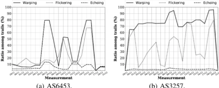
For each target AS, we plot a figure in which we show, for each collected dataset, or snapshot, (X-Axis – snapshot date in DD/MM format), the ratio of trails (Y-Axis) suffering from flickering (dotted line), warping (plain line), and echoing (dashed line). We compute a ratio as the number of trails suffering from a given issue to the total number of discovered trails (the same trail may thus appear multiple times). We do so to avoid under-evaluating warping and flickering in our figures. Indeed, as echoing trails are almost always unique, they would appear as over-represented with a ratio based on unique trails, while, in practice, they appear for much less target IP addresses than both warping and flickering.
2https://github.com/JefGrailet/WISE/tree/master/Dataset/AS6453/2019/02
(a) AS6453. (b) AS3257.
Fig. 2. Examples of problematic trails over time (December 2018). As this paper focuses on typical cases, we encourage readers
to check our public repository 3 to get access to all figures
(but also our scripts and snapshots). Fig. 2a shows the extent of all three issues for AS6453, using snapshots collected from late November 2018 to shortly before Christmas 2018. With the exception of one snapshot collected from a vantage
point that had poor reachability (December 17th), all issues
appear in almost every snapshot. Three spikes (corresponding in practice to six snapshots) are visible and are due to warping trails ratio drastically increasing. Interestingly, the flickering ratio also spikes but only for three of these six snapshots, and stays below 20% (a fairly common observation with this particular AS) for the first “hill” observed for warping trails. This supports the idea that both issues are caused by different kinds of traffic engineering (most probably load-balancing), as we discussed in Sec. II-B.
For the sake of comparison, we also provide results for AS3257 (GTT Communications) in Fig. 2b. Here, a large majority of trails correspond to warping trails, no matter the vantage point (first and last snapshots corresponding to Planet-Lab nodes located at that same geographical location with poor reachability). However, the ratio of trails that corresponds to flickering trails vary a lot from one snapshot to another, further supporting our hypothesis that both warping and flickering are the results of different traffic engineering strategies. We finally note that there is a low, yet noticeable quantity of echoing trails in all snapshots. The weak variations might be simply explained by the fact that the total of responsive interfaces vary from one snapshot to another. Indeed, in the case of AS6453, the small spikes in echoing trails match snapshots that contained more responsive interfaces. In other words, the presence of echoing trails is likely not a consequence of traffic engineering, but rather a matter of what kind of device is used in the surroundings of target addresses.
III. WISE
In order to address carefully the issues described in Sec. II, we introduce a new tool called Wide and lInear Subnet inferencE (WISE). Not only WISE is designed to provide a renewed subnet inference taking account of the issues previously discussed, but it is also designed to discover subnets on wide ranges of IP addresses in a linear time. Indeed, despite using multithreading and sometimes implementing heuristics to speed up subnet inference, state-of-the-art tools such as TreeNET [11] can still require either several days
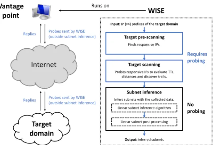
Target pre-scanning
Target scanning Finds responsive IPs.
Probes responsive IPs to evaluate TTL distances and discover trails.
Subnet inference Infers subnets with the collected data.
Linear subnet inference algorithm Linear subnet post-processing Input: IP (v4) prefixes of the target domain
Output: inferred subnets
Requires probing No probing WISE Runs on Vantage point Internet Target domain
Probes sent by WISE (outside subnet inference)
Probes sent by WISE (outside subnet inference) Replies
Replies
Fig. 3. WISE overall design. WISE typically runs from a single vantage point, sending probes over the Internet towards a target domain.
of measurements or several vantage points in order to fully measure a target domain whose prefixes cover several millions of IP addresses. Such an amount of resources can be a problem to schedule large-scale measurement campaigns. This is why
WISE also puts the emphasis on achieving linear complexity
for all its major algorithmic steps (Sec. III-E).
Indeed, given a set of target IPv4 prefixes4 belonging to the
target domain5, WISE works as a succession of three stages:
target pre-scanning (Sec. III-A), target scanning (Sec. III-B), and finally the subnet inference itself, consisting of an offline inference algorithm (Sec. III-C) followed by a short post-processing of the results (Sec. III-D). It is worth noting that the two first stages are the only algorithmic steps requiring active probing. Fig. 3 summarizes the design of WISE as a flow-chart (right) and the typical deployment of WISE (left). For the sake of readability, this paper will summarize the main ideas behind each algorithmic step of WISE. Interested readers can learn more about the implementation details by reviewing
the source code.6
A. Target Pre-Scanning
The first step towards subnet inference, the aggregation of IP interfaces under a single identifier on the basis of their network location, is to check which IP addresses are alive and reachable. This is the objective pursued by “target pre-scanning”: it works by sending a single probe (typically an ICMP one but UDP and TCP can also be considered) with a large enough TTL value towards every possible IP address encompassed by the initial target prefixes and awaiting for a reply. If no reply is received within a given delay, the target address will not be probed in subsequent steps.
In practice, WISE conducts pre-scanning by listing all target addresses, randomizing their order and sharing the probing load between multiple threads in order to speed up the whole process. WISE also does a second pre-scanning with addresses that were unresponsive during the first measurement round. This second run is still scheduled with multiple threads but
4WISEis currently only implemented for IPv4.
5e.g., prefixes listed for the selected AS on http://bgp.he.net
6https://github.com/JefGrailet/WISE/tree/master/v1/
with the initial timeout value being doubled. This ensures unresponsive addresses are indeed dead and not unreachable because of some particular network conditions. Note that
WISEmay allow a third pre-scanning run at user’s will.
B. Target Scanning
Once all live addresses have been found by WISE, the next step consists in collecting the data required for subnet inference (the so-called “target scanning”). For each interface, we are only interested by two pieces of information: an estimation of the distance as a minimal TTL value and its trail, as defined in Sec. II-B. To obtain those details, for every responsive IP address found in the target domain, WISE performs hop-limited probing (i.e., traceroute) and stops when it has received its first reply from the targeted IP address. Then, WISE performs some backward probing to ensure no reply could be obtained closer to the vantage point. For reminders, backward probing consists in (re-)probing a target IP while decrementing the TTL value of the probe packets [25]. Interfaces revealed on the path to the target are used to both estimate the distance in TTL and find the trail.
In practice, because knowing the complete path towards each subnet interface is not useful for the subnet inference step (see Sec. III-C), WISE does not perform a complete
traceroutetowards each target IP address and uses
heuris-tics to minimize the amount of probes. Before the probing, IP addresses are sorted in increasing order, based on their 32-bit integer equivalent. As consecutive addresses could very well be on the same subnet or in the same part of the target network, they might be found at a similar (if not identical) distance. Consequently, when WISE knows the TTL distance required to reach a given IP address, it uses this TTL in the first probe towards the next IP address in the list. Depending on the outcome for this first probe, it will complete the distance estimation and trail discovery by doing some forward/backward probing, minimizing so the total amount of probes sent to IP addresses that are consecutive with respect to the IP scope.
The overall process is further sped up with multithreading, and completed with a second probing round minimizing the amount of situations where the last hops towards a given target address are anonymous. Indeed, anonymous hops can also be the result of temporary network filtering like rate-limiting.
At the end of the target scanning, WISE processes the data collected in order to detect all flickering, warping, or echoing trails. In particular, it will make a census of all flickering trails and group those addresses depending on which addresses they are flickering with. On that basis, it will conduct alias resolution on each group to ensure we are in the scenario described in Sec. II-B. Otherwise, WISE will avoid inferring subnets on the basis of un-aliased flickering addresses. As already mentioned in Sec. II-B, WISE re-uses a fingerprinting-based framework [21], [22] to perform alias resolution. C. Subnet Inference
The subnet inference in WISE consists in processing the scanned IP addresses after sorting them with respect to the IP
scope (i.e., sorted according to their value as a 32-bit integer) to discover the subnets that best accommodate subsets of con-secutive addresses. More precisely, WISE starts by removing an address from the sorted list, builds a /32 subnet for it, then progressively decreases its prefix length and retrieves from the initial list all interfaces that are encompassed by this expanded subnet. It then proceeds to check if encompassed addresses are indeed on the same subnet, and lists aside other addresses as potential contra-pivot(s) or outliers.
To check if an IP address belongs to the current subnet,
WISEfirst selects the first pivot IP address of the initial subnet,
denoted as the reference pivot. Then, the newly encompassed IP addresses, which we will refer to as candidate interfaces, are compared to this reference pivot to ensure both a candidate and the reference interfaces are on the same subnet. To do so,
WISE checks up to five inference rules. All rules have the
same underlying idea: two interfaces, close with respect to the IP scope, can only be on the same subnet if their trails belong to the same device, and, if such a relationship cannot be elucidated, they should at the very least be observed at the same distance while their trails should behave similarly. If both interfaces verify at least one rule, then they will be considered as being part of the same subnet.
The five inference rules are the following:
• Rule 1: both interfaces have the exact same trail.
• Rule 2: both interfaces do not share the same trail, but
are located at the same TTL distance and their trails differ in terms of anomalies (as explained in Sec. II-B).
• Rule 3: both interfaces are located at the same TTL
distance and exhibit echoing trails.
• Rule 4: both interfaces are located at the same TTL
distance and their trails are flickering with each other and previously aliased.
• Rule 5: both interfaces are not located at the same TTL
distance and do not share the same trail. However, trail addresses were aliased during the analysis of flickering IP interfaces, meaning they belong to the same device reached through asymmetrical paths.
It should be noted that rule 2 is a way to ensure that an interface located at the same distance as all other interfaces in a subnet is not eventually wrongly identified as an outlier because its trail could not be discovered accurately (most likely because of a measurement issue, such as rate-limiting or periodical delay). While testing this rule, WISE also considers replacing the reference pivot if the candidate address has a better trail (i.e., less or no anomalies).
When all candidate interfaces have been checked, WISE verifies how many of them were identified on the subnet. Interfaces that are not identified as being on the subnet are classified as potential contra-pivot(s) if they appear closer in terms of distance and as outliers otherwise. If no potential contra-pivot was discovered, WISE keeps expanding as long as outliers are absent or in minority with respect to the whole
set of interfaces. 7 Otherwise, the subnet is shrunk, i.e., its
prefix length is incremented, the shrunk subnet is added to the
7By default, WISE considers outliers a minority if they make up less than
1/3 of the subnet. This can be changed at user’s will upon running WISE.
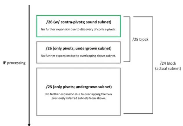
/26 (w/ contra-pivots; sound subnet) No further expansion due to discovery of contra-pivots.
/26 (only pivots; undergrown subnet) No further expansion due to overlapping above subnet.
/25 (only pivots; undergrown subnet) No further expansion due to overlapping the two previously inferred subnets from above.
/25 block
/24 block (actual subnet) IP processing
Fig. 4. Typical case of a subnet being chunked during inference.
results and not encompassed candidate interfaces are restored for the inference of the next subnet.
If contra-pivot(s) are discovered and if pivots remain a majority among interfaces, WISE stops the current inference as the subnet already fulfills the ideal subnet definition pre-sented in Sec. II-A. Doing so allows WISE to correctly infer consecutive subnets (e.g., a succession of /30 subnets found within the same /24 prefix) which the pivot interfaces share the same trail and/or are seen at the same TTL distance, as long as they all feature at least one contra-pivot interface. In the case where there are more contra-pivot interface(s) than pivots overall, the subnet is shrunk to avoid keeping an incoherent subnet among the inference results. Indeed, said contra-pivots are more likely pivot interfaces of another subnet.
WISEwill also shrink and save a subnet if it starts
overlap-ping previously inferred (and potentially sound) subnet(s) upon expansion. Finally, WISE also considers additional specific scenarios during subnet inference (e.g., testing if the selected pivot of a small subnet could be a contra-pivot after all, or testing smaller hypothetical subnets when several contra-pivots appear at once in a large subnet), each one being addressed by a dedicated heuristic. We leave the details of those heuristics
to interested readers.8 We also note that WISE currently does
not expand a subnet beyond the /20 prefix length, as we never observed a /19 during our measurements and as /20 is also the minimum prefix length discussed in previous works on subnet inference [9], [10].
D. Subnet Post-Processing
As WISE stops subnet growth as soon as it finds one or several contra-pivot(s), the positioning of such interfaces among the scope of a subnet can influence the inference results at first. For instance, if WISE discovers the first pivot interfaces and the contra-pivot interface of an actual /24 subnet early enough, it will produce an undergrown subnet (e.g., a /26) and will infer undergrown subnets for the remaining pivots of the actual subnet, as the inference algorithm forbids to grow a subnet further if it starts overlapping a previously inferred subnet. Fig. 4 depicts such a problematic scenario.
Rather than modifying the inference algorithm itself by allowing growth beyond contra-pivot discovery, minimizing so
the risks of overgrowing subnets, WISE mitigates this problem in two ways. First, WISE implements an heuristic that consists in processing backwards the list of IP interfaces during the in-ference. Indeed, many of our observations showed that contra-pivots are usually found among the first subnet addresses. Going backwards therefore ensures we can maximize the size of the inferred subnets as soon as possible.
Second, WISE conducts a short post-processing stage after the inference to aggregate consecutive (i.e., with respect to the address space) subnets that might be chunks of a larger subnet. This stage consists in processing the list of inferred subnets iteratively. Each time WISE comes across a subnet which could not be expanded furthermore (we will refer to it as an undergrown subnet) because it overlapped a previously inferred subnet during the inference, it decrements its prefix length and lists all newly overlapped subnets. It then evaluates whether the overlapped subnets are compatible, i.e., whether any of their interfaces are on the same subnet as the selected pivot of the undergrown subnet, re-using the five rules of inference mentioned previously. If all overlapped subnets are compatible, WISE performs several checks to ensure the subnet which would be obtained by merging them would be sound. It notably ensures that at most one subnet with contra-pivot(s) is listed, not only because having several such subnets would lead to an ill result, but also because it corresponds to the problematic scenario we described before and which the post-processing is meant to solve. WISE also checks if the pivots found in the hypothetical merged subnet are still in majority. If the merging scenario passes all tests, the expansion of the initially undergrown subnet resumes and goes on until a bad merging scenario is encountered or until a /20 is considered. When a bad merging scenario is encountered,
WISE goes back to the previous prefix length, performs the
merging (if any is needed) and looks for the next undergrown subnet in the list of inferred subnets.
It is worth noting that, at the end of post-processing, WISE also performs additional tasks to complete the inference data. In particular, it computes the longest prefix that would contain all interfaces for each incomplete subnet (i.e., missing contra-pivot interface(s)) as aside information. Indeed, a sparse subnet without contra-pivot(s) can feature a prefix larger than what is needed to encompass all its interfaces. WISE also uses an alternative definition of a contra-pivot interface for subnets where the distance of pivot IPs vary considerably: in such a situation, the sole or few IPs(s) which do not have a matching trail are identified as contra-pivot interfaces. WISE does this detection at the very end of post-processing, as a best
effort strategy for subnets where TTL isn’t reliable enough to
identify contra-pivot interfaces.
E. Complexity
We argue that the subnet inference (as described in Sec. III-C) has a linear complexity with respect to the amount of addresses to aggregate in subnets. Indeed, upon evaluating new interfaces of a growing subnet, WISE compares each candidate interface with the reference interface only once. An interface is only compared twice or more when subnet
shrinkage occurs. There are two possible worst cases that could lead to a given interface being compared multiple times. In a first scenario, the network exclusively consists of small subnets featuring only one interface (e.g., a /32 or /31 prefix). Upon expanding the subnet, one or two other IP addresses will be encompassed, but as they will not be compatible with the current interface, they will be put back in the list of interfaces and therefore considered a second or even a third time with the next subnets. Therefore, in this scenario, all addresses are considered up to a bounded amount of three times. In the second worst scenario, the network consists of consecutive subnets whose prefix length progressively increases (e.g., a /25, then a /26, then a /27, etc. all contained in a /24 prefix). Indeed, the last expansion (assuming it occurs) of the first will encompass all other addresses, but as they are on different subnets, they will be put back in the list, after what the same scenario will occur again but on a smaller scale. In the end, the interfaces of the smallest subnet will be compared as many times as they are subnets. As a consequence, the total amount of comparisons is bounded by N + N/2 + N/4 + ... = 2N (where N is the amount of live interfaces considered by the inference). Given that WISE does not go below the /20 prefix, this specific worst case even has an upper bound for the amount of processed interfaces. Therefore, the complexity of subnet inference in WISE is linear.
We also argue that the complexity of post-processing is linear as well. Indeed, the worst case for post-processing would consist in overlapping several times the same sub-nets. The worst possible situation would be to consider a large undergrown subnet followed by a set of consecutive undergrown subnets with a progressively increasing prefix length (e.g., a /24, then a /25, etc. all encompassed in the same /23 prefix). An expansion of the first undergrown sub-net would encompass all subsequent subsub-nets. If merging all subnets does not produce a sound subnet, the first subnet is put back and the same scenario repeats itself with the second subnet and all subsequent subnets. Under the condition that all merging scenario fails, we will evaluate a total of N + (N − 1) + (N − 2) + ... + 1 = N × (N − 1)/2 subnets (where N is the amount of subnets), which is quadratic. However, due to the bounded size of subnets (i.e., max /20 in WISE), the very worst case would be to have a sequence of 12 undergrown and incompatible subnets where the first subnet would be a /21. Assuming evaluating the compatibility of subnets for a merging is in O(1) due to the light operations (e.g., comparing pivots with the five rules of inference), we can therefore consider post-processing to have linear complexity. In practice, as WISE only considers a merging scenario upon finding an undergrown subnet among inferred subnets, post-processing will be a very light step if inference worked well and produced few undergrown subnets.
IV. VALIDATION
In this section, we validate, relying on two ground truth topologies, the ability of WISE to accurately reveal subnets and to perform overall better than state-of-the-art tools.
A. Methodology
To validate WISE, we measured two ground truth topolo-gies with both WISE and a state-of-the-art tool: TreeNET.
TreeNET [11] is a topology discovery tool built upon
ExploreNET [10] that improves its subnet inference and
execution time by adding subnet refinement algorithms and various heuristics. The last version of TreeNET allows one to output inferred subnets before any refinement (providing so topologies as seen by ExploreNET) and after refinement. Doing so, we can compare WISE to both TreeNET and
ExploreNETregarding subnet accuracy in a single shot. We
fully describe our validation approach and provide some useful
scripts in our online repository. 9
Our ground truth networks consist of an academic network, spanning over roughly a /16 prefix (i.e., a bit more than 65,355 addresses), and the backbone of a major Belgian ISP,
encompassing hundreds of thousands of IP addresses. 10 For
each ground truth, we ran both WISE and TreeNET from a single vantage point located inside the academic network and from a PlanetLab node outside of the Belgian ISP, respectively. Both measurements were run in September 2019.
B. Results
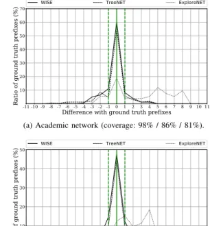
To compare the accuracy and performance of WISE with the state of the art, we introduce the notion of subnet distance, computed as follows: for each subnet prefix in a ground truth, we look for similar subnet prefixes in our data, either identical or overlapping, and compute the difference in bits between the prefix lengths. A subnet distance of 0 corresponds to a perfect inference, meaning the inferred subnet prefix perfectly matches the ground truth prefix. Negative subnet distance values correspond to overgrown subnets, while positive values refer to undergrown subnets.
It is worth mentioning that, in general, we prefer subnet distance to be positive (i.e., undergrown subnets). Indeed, the lack of live interfaces in a part of the subnet address space can prevent the inference of its true prefix length, and therefore, an undergrown subnet can still be faithful to the actual topology. For instance, a /24 sound subnet (i.e., containing both pivots and contra-pivot(s)) where only addresses in the first half are
live will typically be revealed as a /25 by WISE. Overgrown
subnets, on the other hand, typically spans over multiple actual subnets and cannot be considered as faithful to the topology.
To visualize the subnet distance, one can compute the ratios of ground truth prefixes being overlapped by inferred subnets for each possible possible subnet distance and plot a curve where the X-axis gives the subnet distance while the Y-axis gives the ratio of ground truth prefixes matched by inferred subnets for the given subnet distance. Ideally, such a curve should present a peak centered around the subnet distance of 0, therefore corresponding to a perfect inference. It is worth noting that, by design, several undergrown subnets can be overlapped by a same ground truth prefix. To ensure a ground truth prefix is matched to at most one inferred subnet while
9https://github.com/JefGrailet/WISE/tree/master/Evaluation/Validation
10No data for them is provided for security and confidentiality concerns.
-11 -10 -9 -8 -7 -6 -5 -4 -3 -2 -1 0 1 2 3 4 5 6 7 8 9 10 11
Difference with ground truth prefixes
10 20 30 40 50 60 70
Ratio of ground truth prefixes (%)
WISE TreeNET ExploreNET
(a) Academic network (coverage: 98% / 86% / 81%).
-11 -10 -9 -8 -7 -6 -5 -4 -3 -2 -1 0 1 2 3 4 5 6 7 8 9 10 11
Difference with ground truth prefixes
10 20 30 40 50
Ratio of ground truth prefixes (%)
WISE TreeNET ExploreNET
(b) Belgian ISP backbone (coverage: 91% / 89% / 75%). Fig. 5. Subnet distance of inferred subnets on our ground truths.
computing our ratios, we only take the largest undergrown subnet into account in this scenario. Doing so allows us to also compute the overall ratio of ground truth prefixes being matched to any inferred prefix, which we will denote as the ground truth coverage, by summing all ratios together.
Fig. 5 provides the visualization of subnet distance we previously described for both our ground truth networks. The captions of both figures also give the ground truth coverage obtained by WISE (plain line), TreeNET (dashed line), and
ExploreNET(dotted line), in this order. The green vertical
line at subnet distance 0 is a marker for the perfect situation. Additional green dotted lines at subnet distance of -1 and 1 highlight the inferred prefixes differing by at most one bit. Generally speaking, both figures show that WISE is able to reveal more (nearly) exact prefixes than TreeNET, going as far as 60% of exact prefixes on the academic network.
WISE also tends to infer more undergrown subnets (positive
subnet distance) than TreeNET. As explained earlier, this is a desirable result, as undergrown subnets can still be a realistic estimation. Moreover, the coverage achieved by WISE is better in both cases, especially with the academic ground truth. We explain this by the fact that ExploreNET can sometimes discard small subnets due to a lack of live interfaces. Since
TreeNET refines (and expands) subnets initially discovered
by ExploreNET [11], its coverage can improve but some-times at the cost of too overgrown subnets (in the case of the Belgian ISP). Finally, as both our ground truths had few occurrences of flickering or warping IPs, we expect WISE to behave better than other tools in worse contexts.
We now take a look at performance during the subnet inference step of WISE and TreeNET, taking account of the probing stage of WISE which collects the required data (the subnet inference itself being offline). We deliberately
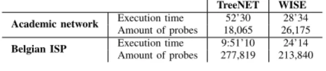
TreeNET WISE Academic network Execution time 52’30 28’34 Amount of probes 18,065 26,175 Belgian ISP Execution time 9:51’10 24’14
Amount of probes 277,819 213,840
TABLE I
PERFORMANCE OFTR E ENETANDWISE.
omit the pre-scanning stage (Sec. III-A) from our comparison because TreeNET uses a similar technique to make a census of live interfaces before its subnet inference. Table I shows the execution time of both TreeNET and WISE on each network as well as the total amount of probes sent by each. In both situations, WISE completes its probing and its subnet inference much faster than TreeNET, and this is especially true on a large network such as the Belgian ISP. Indeed, the subnet inference as performed by TreeNET required hours of execution while WISE only took about half an hour, mostly because TreeNET infers a subnet and probes its interfaces at the same time (the amount of targets increasing with smaller prefix lengths), while WISE performs lightweight probing on the initial live IP addresses at a steady rate, leaving subnet inference for later. The addition of multithreading further increases the gap in execution time, though this also makes
WISE more intensive in terms of probing. Hopefully, this
method of probing remains very reasonable: in the case of the Belgian ISP, WISE sent on average 147 probes per second, which amounts to 8,232 bytes of data, assuming our typical probe is an ICMP probe (32 bytes) encapsulated in an IP packet (24 bytes overhead).
V. EVALUATION IN THEWILD
This section discusses data collected in the wild using the PlanetLab testbed. We use this data to show that WISE can find a good amount of sound-looking subnets in the wild as well as to demonstrate that WISE is able to re-discover the same subnets in a target domain whatever the vantage point location used in a measurement campaign. Our full dataset is
publicly available online.11
A. Subnet Soundness Rules
In the absence of a ground truth to assess the measurements validity, we have to define criteria indicating whether a given subnet is sound or aberrant. Ideally, a subnet should be as close as possible to the ideal definition used by state-of-the-art tools, but we should let room for situations where distances towards pivots (TTL-wise) are not all equal. We therefore define three rules for ensuring the soundness of a subnet: the contra-pivot rule, the spread rule, and the outlier rule.
The contra-pivot rule states that an ideal subnet should feature at least one contra-pivot interface, as a subnet lacking one could be only a part of a larger subnet. The spread rule states that, in the presence of contra-pivots, these interfaces are either in minority for large subnets, either no more common than pivots for small subnets (i.e., the prefix length 29 or greater). Finally, a subnet fulfilling the outlier rule is a subnet containing no other interfaces than pivots and contra-pivots. A subnet satisfying the three rules is considered as sound, and if
11https://github.com/JefGrailet/WISE/tree/master/Dataset
the TTL distances of the pivots are identical while the contra-pivot(s) is (are) found exactly one hop sooner, then the subnet satisfies the ideal definition of previous state-of-the-art subnet inference tools.
It is worth noting that revealing a given subnet prefix from different vantage points does not mean that the prefixes will meet exactly the same soundness rules. For instance, it is always possible that the subnet revealed from vantage point X features an outlier, while the same subnet revealed from vantage point Y will exhibit highly varying distances, making the contra-pivot interface detection difficult (which the final check of post-processing, mentioned in Sec. III-D, attempts to achieve). Our rules are thus also a good indicator on how various vantage points (and, consequently, the different paths towards the targeted domain) can increase the difficulty of inferring a given subnet, notably due to traffic engineering, as discussed in Sec. II.
B. Measurement Methodology
Starting from December 28th, 2018 up to the end of
Febru-ary 2019, we measured 27 different ASes of vFebru-arying sizes (from small stub ASes to large transit ASes covering roughly four millions of IP addresses) from the PlanetLab testbed. To select representative ASes, we relied on a dataset from CAIDA providing the AS class (i.e. Tier-1, Transit, or Stub) [26]
and on the ASRank website 12 also maintained by CAIDA.
We measured again a subset of these ASes 13 in September
2019. Two more campaigns have also been carried out in November and early December 2019, and all three campaigns also collected neighborhood data (see Sec. VI). Each targeted AS has been probed with WISE using a single PlanetLab node at once (located outside of the AS), therefore getting a single dataset (which will also refer to as snapshot), before being re-probed from a different node. Just like in Sec. II-C, we changed of PlanetLab node at each snapshot to eventually assess the effects of measuring a same target domain from different vantage points. This was implemented in practice by doing a rotation of our vantage points after getting the latest snapshot of each measured AS.
C. Observations in the Wild
To assess the soundness of our measurements, we first plot the amount of subnets collected for a given AS over a given period of time and show how many of these subnets fulfill a certain amount of rules (as presented in Sec. V-A). As we measured 27 ASes in early 2019 and a subset of the same ASes in Fall 2019 and scheduled several campaigns, we only focus here on the most typical cases to elaborate on how WISE performs in the wild.
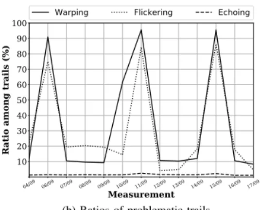
Fig. 6 shows our results for AS6453 with the data collected in September 2019. More specifically, Fig. 6a depicts the amounts of inferred subnets (bottom part) and their sound-ness as ratios (top part) while Fig. 6b shows the ratios of problematic trails observed for the same measurements in the
12http://as-rank.caida.org/
04/09 06/09 07/09 08/09 09/09 10/09 11/09 12/09 13/09 14/09 15/09 16/09 17/09 0 25 50 75 100 % of subnets
3 rules 2 rules 1 rule None
04/09 06/09 07/09 08/09 09/09 10/09 11/09 12/09 13/09 14/09 15/09 16/09 17/09 Dataset 5000 10000 15000 # subnets
(a) Subnets amounts (bottom) and soundness (top, in %).
04/09 06/09 07/09 08/09 09/09 10/09 11/09 12/09 13/09 14/09 15/09 16/09 17/09 Measurement 10 20 30 40 50 60 70 80 90 100
Ratio among trails (%)
Warping Flickering Echoing
(b) Ratios of problematic trails. Fig. 6. Observations made on AS6453 (September 2019).
04/09 06/09 07/09 08/09 09/09 10/09 11/09 12/09 13/09 14/09 15/09 16/09 17/09 0 25 50 75 100 % of subnets
3 rules 2 rules 1 rule None
04/09 06/09 07/09 08/09 09/09 10/09 11/09 12/09 13/09 14/09 15/09 16/09 17/09 Dataset 5000 10000 15000 20000 25000 # subnets
(a) Subnets amounts (bottom) and soundness (top, in %)
04/09 06/09 07/09 08/09 09/09 10/09 11/09 12/09 13/09 14/09 15/09 16/09 17/09 Measurement 10 20 30 40 50 60 70 80 90 100
Ratio among trails (%)
Warping Flickering Echoing
(b) Ratios of problematic trails Fig. 7. Observations made on AS3257 (September 2019).
same manner as in Sec. II-C, for the sake of comparison. Fig. 7) provides the same kinds of figures for AS3257, again using the data collected in September 2019. The first major result highlighted by these figures is that a large majority (>90%) of subnets fulfill at least one rule, and a quick look at the data shows that this rule is usually the outlier rule. In other words, WISE can infer subnets that are free of outliers most of the time. The other result is that the amount of subnets fulfilling all three rules is also considerable, with several snapshots having more than 60% of such subnets in the case of AS6453. The ratios of subnets fulfilling only two rules is fairly low, however, but they all correspond to cases where there is at least one contra-pivot and where the presence of outliers or the amount of contra-pivots violates the
outlier ruleor the spread rule, respectively. Another interesting
result is that WISE is rather constant in terms of soundness despite the varying difficulties encountered with the selected ASes, as shown by Fig. 6b and Fig. 7b. We note, however, that the ratio of sound subnets (i.e., fulfilling all rules) can sometimes face a sudden drop. Interestingly, this drop can correspond to cases where WISE discovered more or less subnets than in previous measurements. As the amount of alive IP addresses did not change much between snapshots, this suggests subnets discovered during previous measurements were actually chunked because of new difficulties induced by additional traffic engineering.
We also take a look at the persistence of subnets across various snapshots. A subnet is said to be weakly persistent if its prefix is present in two snapshots collected from different PlanetLab nodes. It is said to be strictly persistent if both subnets from each snapshot fulfill the same amount of rules (defined in Sec. V-A). A weakly persistent subnet demonstrates two things: first, changing the vantage point from one run of
WISEto another can lead to additional issues as described in
Sec. II-C. Second, this shows WISE can re-discover the same subnets despite these additional issues to a great extent.
Fig. 8 shows the persistence of subnets for the same ASes as before on the same dates, using each time the chronolog-ically first snapshot as reference dataset (i.e., all subsequent snapshots are compared to this first one). The results show that the subnets discovered by WISE have a good persistence overall, with a majority of strictly persistent subnets in both situations for most snapshots. The noticeable amount of per-sistent subnets fulfilling a different amount of rules for each snapshot shows, on the other hand, that each measurement comes with a certain amount of subnets that differs from previous measurements. An interesting observation to make is that the persistent subnets drop (both in the weak and the strict
sense) on September 16th, 2019 for AS3257 correlates with the
drop of subnets fulfilling all rules on the same date (compare Fig. 7a with Fig. 8b). Moreover, the amount of subnets being weakly persistent is noticeably greater than for any other snapshot, supporting so the idea that traffic engineering or measurement issues can both decrease the soundness of the inferred subnets and cause previously measured subnets to appear differently as well. In particular, outliers can appear from one snapshot to another, or warping interfaces can make the distances of both pivots and contra-pivots vary.
06/09 07/09 08/09 09/09 10/09 11/09 12/09 13/09 14/09 15/09 16/09 17/09 Dataset 5000 10000 15000 # subnets (w.r.t. 04/09)
Strictly persistent Persistent No equivalent
(a) AS6453. 06/09 07/09 08/09 09/09 10/09 11/09 12/09 13/09 14/09 15/09 16/09 17/09 Dataset 5000 10000 15000 20000 25000 # subnets (w.r.t. 04/09)
Strictly persistent Persistent No equivalent
(b) AS3257. Fig. 8. Persistence of subnets (September 2019).
To give a practical example, one can look at the sub-net 129.242.88.0/21 WISE regularly discovered in AS224 (UNINETT). In most measurements, the subnet appears with a single contra-pivot and very regular distances (all pivots being located at the same TTL), a result that can be seen in the
snapshots collected on February 2nd, 2019 and September 4th,
2019. However, on February 8th and February 10th, the same
subnet appeared with highly varying TTLs, with the former snapshot having pivots at respectively 16 or 18 hops and the latter at 21 and 24 hops. A similar change was observed on
September 15th, where the pivots were this time found at either
20 or 21 hops from the vantage point. Hopefully, the contra-pivot always appearing sooner, all inferred subnets remained sound with respect to our usual criteria.
Overall, our measurements show that, while choosing the vantage point is still important to maximize accuracy of the subnet inference, a tool such as WISE can mitigate pretty well traffic engineering issues with a few exceptions. Due to the variety and quantity of results, we encourage readers to
take a look at our public repository 14 to see all figures. In
particular, we also provide figures showing the distribution of subnet prefix lengths in our snapshots. These additional figures demonstrate WISE can discover all kinds of prefix length though the distribution of these lengths will usually follow a power-law shape (/30 and /31 being the most common prefixes), as already showed by previous research [10].
VI. TOPOLOGYINFERENCE
In this section, we discuss the potential for inferring a comprehensive map of the target domain by taking advantage
14https://github.com/JefGrailet/WISE/tree/master/Evaluation
Trail (same for all subnets)
Route hops observed before the trail
L2 / L3 mesh
Subnet ingress (i.e., contra-pivot)
Neighborhood
Subnet S1
Subnet S3
Subnet S2
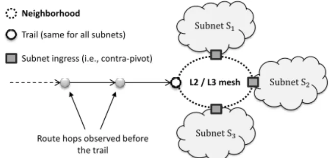
Fig. 9. An illustration of the concept of neighborhood.
of the subnet data inferred by WISE. Sec. VI-A first presents the key concepts (in particular, the notion of neighborhood) one could use to achieve this and briefly reviews the net-work modeling they could lead to. Then, Sec. VI-B briefly explains how we modified WISE in order to integrate those concepts and collect neighborhood data. Sec. VI-C discusses the soundness of the concept of neighborhood by confronting inference results with the same ground truth networks as in Sec. IV. Finally, Sec. VI-D analyzes data collected from the PlanetLab testbed in Fall 2019 to demonstrate the viability of
neighborhoodsand associated concepts. Again, all our scripts
are available in our online public repository15.
A. Concepts
A first key observation one can make when looking at subnet data is how often a group of subnets share an identical
trail (outside subnets built around the 3rd rule of inference –
see Sec. III-C). In fact, this observation suggests that such subnets are located close to each others: since their trails are identical, and as the trail is typically provided by an IP interface discovered with traceroute-like probing, then these subnets are all accessed via a same last-hop router which is at the very least part of a mesh bordered by these subnets. We call such a place a neighborhood. We formally define a neighborhood as a network location bordered by a group of subnets at most at one hop apart from each other. In practice, we infer that subnets are one hop away from each other if they have the same trail, and the so-called “network location” can actually consist of either a single router, either a mesh of routers that could also be implemented with Layer-2 devices (e.g., Ethernet switches). Fig. 9 depicts the concept of neighborhood, with the dashed oval modeling
the neighborhood bordered by subnets S1, S2, and S3, all
having the same trail.
The concept of neighborhood has, in fact, been already introduced and put to practice by previous research. Indeed, as sound subnets usually have at least one contra-pivot interface that should be located on the ingress router (i.e., the router providing access to the subnet), then contra-pivot interfaces belong to the single router or the mesh of routers which is first identified as a neighborhood. If we list all such interfaces along with the trail of the subnets, we obtain a handful of good can-didates for alias resolution which can be excluded from being
15https://github.com/JefGrailet/WISE/tree/master/Evaluation/
N
bN
aTrails Subnet ingress (i.e., contra-pivot)
Neighborhood
ta tb
Previous hops
Fig. 10. The concept of (neighborhood) peer. Nb is a (direct) peer of Na
because tb appears before ta in the routes towards pivot IPs of subnets
bordering Na.
aliased with any other live IP addresses observed in the target domain. Discovering neighborhoods therefore acts as a form of space search reduction for alias resolution. TreeNET [11], [22] explored this idea by collecting traceroute records towards inferred subnets in order to build a tree-like map of the target network, designed to infer neighborhoods, therefore to discover sets of alias candidates. One can then perform alias resolution on each set by using fingerprinting [21] to identify the most suitable alias resolution technique among a selection of state-of-the-art methods (such as Ally [23] and iffinder [24]). Alias resolution based on fingerprinting is still being used in WISE upon investigating flickering IP addresses, as explained in Sec. III-B.
We however argue that neighborhoods are not only useful for alias resolution, but also to infer the whole topology of the target domain. Using limited information, it is indeed possible to infer how neighborhoods are located with respect to each other, using the notion of peer. In the context of a neighborhood-based topology discovery, for a given
neighbor-hood Na with a trail denoted ta, a second neighborhood Nb
with trail tb is a peer of Na if and only if tb appears prior
to ta in the routes towards pivot IP addresses of the subnets
bordering Na. In an ideal situation where trails are
anomalies-free (i.e., no cycles or anonymous hops were observed), this means that, in practice, the last two hops before pivot IP
interfaces of the subnets surrounding Na are tb, ta in the
same order. In a less ideal situation where there would be
intermediate hops between tb and ta (for instance) and no
possible tc belonging to a third neighborhood in between, we
say that Nb is a remote peer of Na. On the opposite, when
there are no intermediate hops between tb and ta, we say that
Nb is a direct peer of Na. Fig. 10 depicts the concept of
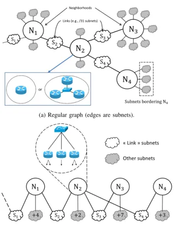
neighborhood peer, using a direct peer for the example. By discovering all neighborhoods within a target network and their respective peers, it could be possible to build a neighborhood-based graph of the target domain. In particular, one can infer the subnets acting as links between the neighbor-hoods, notably by identifying the subnet encompassing a trail associated to a given neighborhood and which neighborhood it belongs to. Doing so, one can even consider a bipartite
model16where one set (or party) gathers neighborhoods while
the second gathers the subnets which connect the
neighbor-16A bipartite graph is a graph in which vertices can be divided into two
disjoint sets, > and ⊥, such that every edge connects a vertex in > to one in ⊥. Bipartite graphs are a fundamental object in computer science and, as such, are widely studied [27], [28], [29].
Neighborhoods
Links (e.g., /31 subnets)
or
N
1N
2N
4N
3 Subnets bordering N4 S1 S 2 S3 S4(a) Regular graph (edges are subnets).
N1 N2 N3 N4
S2 S3 S4
S1 +4 +2 +7 +3
« Link » subnets Other subnets
(b) Bipartite graph (double shown for N2).
Fig. 11. A toy network, viewed with a neighborhood-based perspective. In
both models, what N2could consist of (L3/L2) is shown.
hoods. Such a model can be further deepened by inferring the router(s) found inside the neighborhoods via alias resolution. Then, the set of the neighborhoods can be replaced with a new party of routers (Layer-3), itself being part of a second bipartite graph where the other set consists of the hypothetical Layer-2 devices that glue the routers found in a same neighborhood into meshes. Individual routers can be matched to the subnets depending on the contra-pivot interfaces they bear. A L2-L3 bipartite model of computer networks has already been proposed in the past [15], but had to tie routers not connected via a L2 device with imaginary L2 devices. Starting with a neighborhood-based model can overcome this limitation thanks to subnets, in addition to highlighting the places in the network where L2 equipment might be present. Fig. 11 shows a toy network viewed from a neighborhood-based perspective, first seen as a graph where neighborhoods are vertices while subnets act as edges (Fig. 11a), then as a (double) bipartite graph (Fig. 11b). Both figures show the hypothetical devices
corresponding to the neighborhood N2 (or any other), to be
discovered via alias resolution.
However, before going as far as building bipartite models of the Internet, we first assess the viability of both the concept of neighborhood and the concept of peer. In particular, we have to ensure we can find direct peers that could be used to locate neighborhoods next to each other most of the time. We therefore upgraded WISE such that it can also discover neighborhoods and their peers after first discovering subnets.
B. WISE Upgrade
Neighborhood inference in WISE starts at the end of the subnet inference, i.e., after subnet post-processing (as de-scribed in Sec. III-D). In order to properly discover neigh-borhoods and their peers, WISE first collects additional data: routes towards subnets that are long enough for discovering potential peers. This is done in two steps: first, WISE makes a census of all IP interfaces appearing in anomalies-free trails for pivot IP addresses from any subnet it inferred. We will refer subsequently to these IP addresses as peer IPs. Second, WISE
selects, in each subnet, up to five pivot IP interfaces17towards
each it will perform a backwards partial Paris traceroute, i.e., WISE starts by sending a probe with a TTL value adjusted to reveal the route hop just before the trail of the target IP address, then checks if the resulting interface is a peer IP, excluding this possibility if said interface is identical to the trail IP or an alias of said trail IP. If the interface is not a peer,
WISEsends a new probe with a decreased TTL value. WISE
will only perform a full traceroute measurement if the route towards some target IP address has no peer IP at all. In an ideal situation where the peer is direct (as explained at the end of Sec. VI-A), the partial route only consists of one additional hop: the peer IP. Thanks to this design, WISE collects just enough data for neighborhood inference, minimizing so the amount of probes and the execution time, further sped up with multithreading.
Like the subnet inference itself (Sec. III), the rest of neigh-borhood inference is done entirely offline, in two simple steps: subnet aggregation and peer discovery. The subnet aggregation simply consists in gathering together subnets sharing the same trail, and if not, applying a best effort strategy that will approximate the notion of neighborhood. In practice, WISE goes through the list of subnets and puts them in a map (e.g., a hashmap with O(1) access) on the basis of their associated
trail, except for subnets built with the 3rd inference rule
(echoing trails, see Sec. III-C) which gets another treatment afterwards. After this processing, each list of subnets (one per trail) is equivalent to a neighborhood. For flickering trails, we also further gather together lists corresponding to
previously aliased trails. For the subnets built on the 3rdrule,
WISEfurther separates them based on their typical pivot TTL
distance but also the non-anonymous IP addresses appearing before their trails, as a best effort approximation of what the neighborhood may have looked like if there was no echoing.
Once subnets are aggregated into neighborhoods, WISE ends with the so-called peer discovery. For each neighborhood,
WISE takes a look at the routes towards pivot IP interfaces
and makes a census of all peer IPs at the first hop before the trail. If no peer IP can be found, it then looks at the second hop before the trail, and so on and so forth. As soon as WISE has to look beyond the first hop before the trail, the peers it will discover will not be direct. Peer discovery stops as soon as at least one peer IP is discovered, whether it is a direct peer or not, or when the routes have been completely reviewed, in which case the neighborhood is considered as having no peers.
17Five is a default value chosen to have representative routes for large
subnets; it can be modified when running WISE.
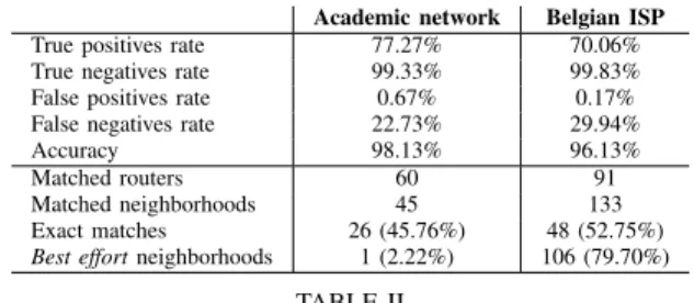
Academic network Belgian ISP True positives rate 77.27% 70.06% True negatives rate 99.33% 99.83% False positives rate 0.67% 0.17% False negatives rate 22.73% 29.94%
Accuracy 98.13% 96.13%
Matched routers 60 91
Matched neighborhoods 45 133 Exact matches 26 (45.76%) 48 (52.75%) Best effortneighborhoods 1 (2.22%) 106 (79.70%)
TABLE II
VALIDATION OF OUR NEIGHBORHOODS(GROUND TRUTH NETWORKS).
C. Observations on the Ground Truth Networks
In order to ensure the concept of neighborhood is sound with respect to actual networks, we confronted new measurements (from late September 2019) with the same ground truth networks as in Sec. IV, with a change: we probed this time the whole Belgian ISP rather than just its backbone. Our partners provided us, for each network, a list of all IPv4 prefixes associated to each router. By comparing the first IP addresses of these prefixes with the first IP addresses of our subnets, we can match the majority of prefixes with our inferred subnets and check how many prefixes associated to a given router were found around the same neighborhood. For the sake of completeness, we also asked our partners to provide us details on how routers were grouped in their network, since a neighborhood can conceptually consist of several devices.
To validate our neighborhood discovery, we consider every possible pair of prefixes identified in both the ground truth networks and our measurements and classify them. A pair found both around the same router ID (or distinct IDs from a known group) and the same neighborhood is classified as a true positive. A pair appearing around the same neighborhood but not around the same router (or group) is a false positive. Likewise, two prefixes that are not around the same router (or group) nor around the same neighborhood constitute a true negative, and a pair found around a same router (or group) but not around the same neighborhood is categorized as a false negative. To complete our analysis, we also define an
exact match as a router whose all prefixes exactly appear in
the same inferred neighborhood. Finally, due to the Belgian ISP ground truth network having a high amount of echoing devices, lots of subnets found within it were discovered
through the 3rdsubnet inference rule, and, consequently, most
of its neighborhoods were built with a best effort strategy (as discussed in Sec. VI-B). We therefore define the best effort
ratioas the ratio of neighborhoods built with such a strategy
or around a trail including anomalies (e.g., anonymous hops). Table II provides the results of our validation. The first major result is the very low false positives rate: less than 1% in both situations, therefore showing the concept of neighborhood and how we infer it so far will rarely produce aberrant results with respect to the topology. On the contrary, as demonstrated by the false negatives rate, it is a rather pessimistic one, yet it can be reasonably trusted with 77% of true positives for the academic network and 70% for the Belgian ISP. Careful analysis of our measurements showed that false negatives are typically the results of incomplete subnets that are missing from large neighborhoods due to measurement issues. For instance, a subnet can be observed through an unique path
(therefore having a unique trail), or with a trail that includes anomalies due to network delays at the time of measurements. Moreover, in some situations, only the contra-pivot interface of the subnet has been seen during the measurements, and falsely identified as a pivot interface. As a consequence, if the subnet is not associated to a new neighborhood, it will be erroneously associated to another neighborhood, creating some false positives. Nevertheless, the results of our validation demonstrate that our inference offers a first good approxima-tion of the topology, with around half of the devices being matched exactly with one neighborhood in both situations. This is especially a good result in the case of the Belgian ISP: as almost 80% of the neighborhoods were inferred with
best effortstrategies, the regular (and allegedly more reliable)
approach could not have been used, and this shows that best
effort methodology can be a good approximation too.
D. Observations in the Wild
We now assess the viability of the concept of peer by reviewing the peers discovered for the neighborhoods inferred by WISE during our latest measurement campaigns from the PlanetLab testbed. In particular, we want to evaluate the poten-tial of such a concept for locating discovered neighborhoods with respects to each others, which would constitute a first step towards the construction of a comprehensive map of the target domain as discussed in Sec. VI-A. To do so, we evaluate respectively the typical distance between a neighborhood and its peers (in terms of hop count) and the typical amount of peers (as individual IPs) for a neighborhood.
We first evaluate the typical distance between a neigh-borhood and its peers, as a difference in TTL which exists between the trail associated to the neighborhood and the first peer IP(s). A TTL difference of 1 means the peer(s) are direct, i.e., the neighborhood is right next to them. A higher TTL dif-ference means there are unseen intermediate hops between the neighborhood and its peer(s). Ideally, we should have as many direct peers as possible, as the opposite would mean we have an incomplete picture of the target AS – unless said AS is split in several components that are not connected to each others. To do so, we processed all the neighborhood data collected for all snapshots for a given AS and a given campaign and computed the ratios of neighborhoods for each difference of TTL, from 1 to the highest difference observed in the data. As our data contains a noticeable amount of neighborhoods containing a single incomplete subnet (often the result of a measurement issue), we weighed each neighborhood by their amount of aggregated subnets while computing our ratios. This means in practice that, if we have for instance a ratio of 85% of direct peers (TTL difference of 1), there is an equal chance that the neighborhood bordered by a subnet picked at random will have direct peers. Finally, we stacked the ratios to produce a Cumulative Distribution Function (CDF).
Fig. 12 shows such a CDF for AS6453, using 12 snapshots
collected for it from November 19th, 2019 to December 6th,
2019. The CDF shows two interesting results. First, for a subnet picked at random, there is a likelihood a bit higher than 90% that the neighborhood it borders will have direct
0 1 2 3 4 5 6 7 8 9 10 11 12 13 14 15
Distance in TTL between neighborhoods and peers
0.1 0.2 0.3 0.4 0.5 0.6 0.7 0.8 0.9 1.0
CDF with weighed neighborhoods
Fig. 12. CDF of the difference in TTL between a neighborhood and its
peer(s), using data collected for AS6453 (12 snapshots in Fall 2019).
1 101 Amount of peers 0.1 0.2 0.3 0.4 0.5 0.6 0.7 0.8 0.9 1.0
CDF with weighed neighborhoods
Fig. 13. CDF of the amount of peers of a neighborhood bordered by a random subnet, using data collected for AS6453 (12 snapshots in Fall 2019). peers, meaning the concept of peer is indeed viable in this context. Second, the curve does not reach 1 at the end. This means that there is a small probability for a random subnet to border a neighborhood that has no peer. In practice, such a neighborhood is usually one of the closest neighborhoods with respect to the vantage point, or to put it in another way, one of the entry points of the target network from the perspective of the vantage point. A neighborhood without peers can also be an ill measurement or simply an isolated component of the target domain. Similar CDFs were computed for other ASes
probed during the same campaign, all available online18, and
usually show a chance between 80% of 90% for a random subnet to border a neighborhood with direct peer(s).
We computed a second kind of CDF with the same data and methodology, but instead of showing the typical difference in TTL between a neighborhood and its peers, we show the typical amount of peers. Fig. 13 shows the result for AS6453 with the same data as for Fig. 12. The curve shows that there is only a probability between 60% and 70% that the neighborhood bordered by a subnet randomly picked will have a single peer. In other words, neighborhoods with multiple peers are not uncommon or have a considerable place in the topology of the target domain, which implies that they are reached from the vantage point through multiple paths. In practice, as peers consist of single IP addresses at this stage of the discovery, one should ideally use alias resolution when confronted to a neighborhood with several peers in order to tell whether these peers belong to separate devices or to a same one. In the second case, said device could therefore be a convergence point in a load-balancing architecture (much like
18https://github.com/JefGrailet/WISE/tree/master/Evaluation/