Crop choices in micro-econometric multi-crop models: modelling corners, kinks and jumps

HAL Id: hal-02983249

https://hal.inrae.fr/hal-02983249

Preprint submitted on 29 Oct 2020

HAL is a multi-disciplinary open access

archive for the deposit and dissemination of sci-entific research documents, whether they are pub-lished or not. The documents may come from teaching and research institutions in France or abroad, or from public or private research centers.

L’archive ouverte pluridisciplinaire HAL, est destinée au dépôt et à la diffusion de documents scientifiques de niveau recherche, publiés ou non, émanant des établissements d’enseignement et de recherche français ou étrangers, des laboratoires publics ou privés.

Distributed under a Creative Commons Attribution - NonCommercial - NoDerivatives| 4.0 International License

modelling corners, kinks and jumps

Obafemi Philippe Koutchade, Alain Carpentier, Fabienne Femenia

To cite this version:

Obafemi Philippe Koutchade, Alain Carpentier, Fabienne Femenia. Crop choices in micro-econometric multi-crop models: modelling corners, kinks and jumps. 2020. �hal-02983249�

Crop choices in micro-econometric multi-crop models:

modelling corners, kinks and jumps

Obafèmi Philippe KOUTCHADÉ, Alain CARPENTIER, Fabienne FÉMÉNIA

Working Paper SMART – LERECO N°20-09

October 2020

Paper published in the American Journal of Agricultural Economics DOI: https://doi.org/10.1111/ajae.12152

UMR INRAE-Agrocampus Ouest SMART - LERECO

Les Working Papers SMART-LERECO ont pour vocation de diffuser les recherches conduites au sein des unités SMART et LERECO dans une forme préliminaire permettant la discussion et avant publication définitive. Selon les cas, il s'agit de travaux qui ont été acceptés ou ont déjà fait l'objet d'une présentation lors d'une conférence scientifique nationale ou internationale, qui ont été soumis pour publication dans une revue académique à comité de lecture, ou encore qui constituent un chapitre d'ouvrage académique. Bien que non revus par les pairs, chaque working paper a fait l'objet d'une relecture interne par un des scientifiques de SMART ou du LERECO et par l'un des deux éditeurs de la série. Les Working Papers SMART-LERECO n'engagent cependant que leurs auteurs.

The SMART-LERECO Working Papers are meant to promote discussion by disseminating the research of the SMART and LERECO members in a preliminary form and before their final publication. They may be papers which have been accepted or already presented in a national or international scientific conference, articles which have been submitted to a peer-reviewed academic journal, or chapters of an academic book. While not peer-reviewed, each of them has been read over by one of the scientists of SMART or LERECO and by one of the two editors of the series. However, the views expressed in the SMART-LERECO Working Papers are solely those of their authors.

1

Crop choices in micro-econometric multi-crop models:

modelling corners, kinks and jumps

Obafèmi Philippe KOUTCHADÉ

INRAE, UMR1302 SMART-LERECO, 35000, Rennes, France

Alain CARPENTIER

INRAE, UMR1302 SMART-LERECO, 35000, Rennes, France

Fabienne FEMENIA

INRAE, UMR1302 SMART-LERECO, 35000, Rennes, France

Paper published in the American Journal of Agricultural Economics DOI: https://doi.org/10.1111/ajae.12152

Acknowledgements

This research has received funding from Arvalis - Institut du végétal and has benefited from financial support by the MINDSTEP project, funded by the European Union’s Horizon 2020 research and innovation programme under grant agreement No 817566.

Corresponding author Fabienne Femenia

UMR SMART-LERECO, INRAE, 4, Allée Adolphe Bobierre

35011 Rennes, France

Email : Fabienne.Femenia@rennes.inra.fr

Téléphone / Phone : +33 (0)2 23 48 56 10 Fax : +33 (0)2 23 48 53 80

Les Working Papers SMART-LERECO n’engagent que leurs auteurs.

2 Crop choices in micro-econometric multi-crop models:

modelling corners, kinks and jumps

Abstract

Null crop acreages raise pervasive issues when modelling acreage choices with farm data. We revisit these issues and emphasize that null acreage choices arise not only due to binding non-negativity constraints but also due to crop production fixed costs. Based on this micro-economic background, we present a micro-econometric multi-crop model that consistently handles null acreages and accounts for crop production fixed costs. This multivariate endogenous regime switching model allows for specific crop acreage patterns, such as multiple kinks and jumps in crop acreage responses to economic incentives, that are due to changes in produced crop sets. Currently available micro-econometric multi-crop models, which handle null acreages based on a censored regression approach, cannot represent these patterns.

We illustrate the empirical tractability of our modelling framework by estimating a random parameter version of the proposed endogenous regime switching micro-econometric multi-crop model with a panel dataset of French farmers. Our estimation and simulation results support our theoretical analysis, the effects of crop fixed costs and crop set choices on crop acreage choices in particular. More generally, these results suggest that the micro-econometric multi-crop model presented in this article can significantly improves empirical analyses of multi-crop supply based on farm data.

Keywords: acreage choice, crop choice, endogenous regime switching, random parameter models

3 Choix des cultures et solutions en coin dans les modèles micro-économétriques de choix

de production multiculture

Résumé

Les surfaces de culture nulles soulèvent de nombreuses questions lorsque l’on souhaite modéliser les choix d’assolement des agriculteurs à partir de données individuelles. Nous revisitons ces questions en mettant en avant le fait que les choix de surfaces nulles ne sont pas uniquement dus à des contraintes de non-négativité saturées mais également à des coûts fixes de production des cultures. A partir de ce cadre micro-économique, nous présentons un modèle micro-économétrique multiculture permettant de représenter de façon cohérente les choix surfaces nulles et tenant compte des coûts fixes de production des cultures. Ce modèle multivarié à changement de régime endogène offre la possibilité de représenter des schémas de choix d’assolement spécifiques, présentant notamment de multiples sauts et points d’inflexion dans les réponses des assolements aux incitations économiques en raison de changements dans les ensembles de cultures produites. Les modèles économétriques multicultures disponibles actuellement, qui tiennent compte des surfaces nulles à partir d’approches basées sur des régressions censurées, ne permettent pas de représenter ce type de schéma.

Nous illustrons la tractabilité empirique de notre approche en estimant, sur un panel d’agriculteurs français, une version à paramètres aléatoires du modèle micro-économétrique multiculture à changement de régime endogène que nous proposons. Nos résultats d’estimations et de simulations viennent appuyer notre analyse théorique, concernant en particulier les effets des coûts fixes de production des cultures et des choix d’ensembles de cultures produites sur les choix d’assolement. Plus généralement, le modèle micro-économétrique multiculture présenté ici peut améliorer significativement les analyses empiriques d’offre de culture basées sur des données individuelles d’exploitation.

Mots-clés : choix d’assolement, choix de culture, changement de régime endogène, modèle à paramètres aléatoires

4 Choix des cultures et solutions en coin dans les modèles micro-économétriques de choix

de production multiculture

1. Introduction

Market prices and agricultural policies impact crop supplies through their effects on input uses and yield levels, and acreage choices. Starting in the eighties with the pioneering work of Just

et al. (1983), Chambers and Just (1989) and Chavas and Holt (1990), agricultural production

economists developed micro-econometric multi-crop (MEMC) models for analyzing and quantifying these effects with farm accountancy data. These models have then been widely applied during the last decades.

In MEMC models, farmers are assumed to allocate their cropland to the crops of a given crop set in order to maximize their expected profit or the expected utility of their profit. This ensures the economic consistency of the resulting models. However, currently available MEMC models ignore or poorly describe an important decision of crop producers: their choice to produce a subset of crops among the set of crops they can produce and sell. Indeed, applications of MEMC models frequently ignore null acreages by relying either on very specific farm samples (e.g., Just et al., 1983, 1990; Bayramoglu and Chakir, 2016) or on crop aggregation that eliminate null crop acreages (e.g., Oude Lansing and Peerlings, 1996; Serra et al., 2005; Oude Lansink, 2008; Carpentier and Letort, 2012, 2014).1 Yet, sample selection prevents extrapolation of the estimation results to farmers not producing all considered crops while crop aggregation induces information losses regarding production choices at the crop level.

A few recent MEMC models explicitly account for null crop acreages (e.g., Sckokai and Moro, 2006, 2009; Lacroix and Thomas, 2011; Bateman and Fezzi, 2011; Platoni et al., 2012).2 These models are designed as censored regression (CR) systems and are estimated following two-step approaches inspired by that initially proposed by Shonkwiler and Yen (1999). These MCEM based on censored regressions (CR-MCEM) suitably account for null acreages from a statistical viewpoint but display severe micro-economic inconsistencies.

1 _{Other applications rely on aggregated data in which the occurrence of null acreages is limited (e.g., Chavas and}

Holt, 1990; Moore and Negri, 1992; Coyle, 1992, 1999; Ozarem and Miranowski, 1994; Guyomard et al, 1996). Such applications are now less frequent thanks to increasing availability of micro-data.

5 Indeed, these models are conceived as statistical versions – featuring error terms and accounting for mass points at 0 – of theoretical micro-economic models ignoring null acreages. Their main shortcoming is due to their relying on a single crop acreage choice model, whatever the subset of crops actually produced. These models thus fail to recognize that the crop acreage choices of a farmer structurally depend on the composition of the set of crops actually produced by this farmer. For instance, farmers are unlikely to consider the prices of the crops they don’t produce when choosing the acreages of the crops they produce.3 Of course, the lack of micro-economic coherency of CR-MCEM models substantially undermines their ability to yield consistent estimates of crop acreage responses to economic incentives. The composition of the produced crop sets, which displays substantial variability when null acreages are frequent, deeply impacts the structure of farmers’ crop acreage choices. These effects of farmers’ crop set choices are ignored in CR-MCEM models.

The recent articles addressing the issue raised by null crop acreages from a statistical viewpoint by considering CR-MEMC models don’t focus either on corner solutions in acreage choices or on farmers’ crop choices. By contrast, the main objective of this article is to develop a consistent modelling framework for analyzing farmers’ crop set choices and, as a result, for handling null crop acreages in MEMC models. More precisely, the main aims of this article are (a) to revisit the null acreage issue in multi-crop models from a theoretical viewpoint, (b) to propose an original MEMC model that accounts for farmers’ crop choices in a way that is consistent from an economic viewpoint, together with a suitable estimation approach, and (c) to show, by means of an empirical application focused on crop diversification choices, that considering crop set choices significantly enriches micro-econometric analyses of farmers’ crop supply.

Our multi-crop micro-economic modelling framework is based on an expected profit maximization problem considering land as an allocable quasi-fixed input. This problem includes the usual crop acreage non-negativity constraints but also production regime fixed costs. The production regime chosen by a farmer is defined by the subset of crops that this farmer decides to plant. The regime fixed costs consist of unobserved costs – such as unmeasured marketing costs or implicit labor and machinery management costs – that depend on the set of crops that are grown but that don’t depend on the acreages of these crops.

3 _{They don’t in a static framework although they might in a dynamic one. For instance, forward looking farmers}

consider (future) prices of crops they don’t currently produce if they plan to produce these crops in the future and if their current crop acreage choices impact their future expected profits (e.g., due to crop rotation effects). Yet, if they cannot be ruled out, these (indirect) effects of the non-produced crop prices are likely to be limited.

6 Accordingly, our modelling framework assumes that farmers choose the production regime maximizing their expected profit, regime fixed costs included, as well as the related optimal crop acreage, yield and input use levels. Importantly, our considering regime fixed costs implies that null acreages are not necessarily due to binding non-negativity constraints.

Based on this micro-economic background, we design our MEMC model as an endogenous regime switching (ERS) multivariate model with multiple regimes. This endogenous regime switching micro-econometric multi-crop (ERS-MEMC) model consists of a probabilistic regime choice model coupled with a set of regime specific MEMC models. As estimating multivariate ERS models with multiple regimes is challenging and considering regime specific fixed costs increases the estimation burden, choosing relevant functional forms for the per regime MEMC models appears crucial. Thanks to their specific properties, the Multinomial Logit (MNL) acreage choice models proposed by Carpentier and Letort (2014) are particularly well suited in that respect. They yield simple and well-behaved functional forms for important components of our ERS-MEMC model, thereby significantly reducing its estimation cost. Relying on the MNL acreage choice models also enables us, following Koutchadé et al. (2018), to go one step further and to account for farmers’ unobserved heterogeneity by considering a random parameter version of our ERS-MEMC model. Estimating ERS models with multiple regimes is challenging mostly because their likelihood function involves integration of expectations over the probability distribution of multivariate latent error terms (e.g., Pudney, 1989).4 Also, the likelihood function of our ERS-MEMC model needs to be integrated over the probability distribution of its random parameters. Our estimation approach combines tools from the micro-econometrics and computational statistics literatures.

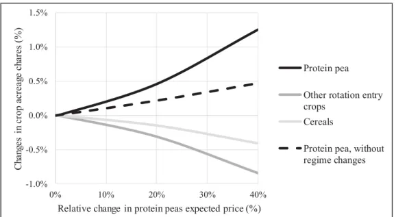
We illustrate the empirical tractability of our approach by estimating our model for a panel data sample of French arable crop producers. Our results tend to demonstrate that our random parameter ERS-MEMC model performs well according to standard fit criteria. They also tend to show that regime specific fixed costs significantly matter in farmers’ crop choice, along with crop expected returns. Importantly, these results also demonstrate that acreage choices’ responses to economic incentives strongly depend on the production regime choices. The elasticity of crop acreages in crop prices increases in the number of produced crops, a pattern that cannot be reproduced by CR-MEMC models. Finally, our simulation results show that the

4 _{In particular, the probability function of the production regime choice of our model cannot be integrated}

analytically. We also have to overcome the fact that the crop yield and input use (and, thus, expected crop return) levels of the crops that are not produced are unobserved.

7 acreage of minor crops respond non-linearly to increases in their prices due to production regime changes.

Our contributions are twofold. First, ERS-MEMC model presented in this article accounts for null crop acreages while relying on a well-defined micro-economic background. As a result, it is the first theoretically coherent response to an issue that is pervasive when analyzing crop production with farm level data. Other ERS-MEMC models could be considered, but the one presented here allows to consider production regime fixed costs as well as farm specific parameters while remaining empirically tractable. Second, this model allows to disentangle the effects of the main economic drivers of farmers’ crop supply choices. It accounts for intensive and extensive margin choices, including the effects on crop set choices at the extensive margin. This unique feature is of special interest for investigating future agri-environmental policies. In particular, owing to its positive agronomic effects, crop diversification is a key feature of environmentally friendly crop production systems (e.g., Matson et al., 1997; Tilman et al., 2002; Lin, 2011; Kremen et al., 2012; Bowman and Zilberman, 2013). Our modelling framework is especially well-suited for analyzing samples containing both specialized and diversified farms as well as for simulating the effects of policy instruments aimed to foster crop diversification.

The rest of this article is organized as follows. The approach proposed to account for crop choices in micro-economic models of acreage decisions is presented in the first section. The structure of the corresponding ERS-MEMC model is described in the second section. The main features of our estimation strategy are presented in the third section, with a specific focus on the main issues arising with random parameter ERS-MEMC models.5 _{Illustrative estimation}

and simulation results are provided in the fourth section. Finally, we conclude.

2. Regime switching in multi-crop acreage models: corners, kinks and jumps

This section presents the theoretical modelling framework we propose for dealing with null crop acreages in micro-econometric acreage choice models. We proceed in three steps. First, we present the micro-economic crop acreage choice model underlying our ERS-MEMC model. Second, we compare this model to the models that have been proposed for modelling multiple

5 _{The overall structure of our estimation procedure is described in the Appendix. A detailed description is given in}

8 binding non-negativity constraints or regime switching. We focus on the ability of these models to cope with corners, kinks and jumps in farmers acreage choices.6 Third, we present the functional form of the crop acreage choice models used in our ERS-MEMC model.

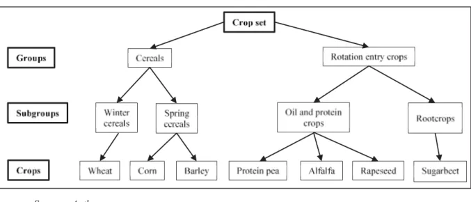
2.1. Crop choices and crop acreages

We assume that farmers can allocate their fixed cropland area to K crops. Accordingly, set

{1,...,K} =

K denotes the set of crops that any considered farmer can produce and sell and farmers’ problem consists of optimally choosing a crop acreage share vector

_s

=

_{( :}

_{s k}

_k

Î

_K

₎

satisfying s³0 and s ι¢ =1, term ι _{being the dimension K unitary column vector.}

We now introduce notions and notations aimed at describing farmers’ decisions to produce a subset of crops among crop set

K

. Set R ={1,..., }R denotes the set of feasible production regimes. A production regime is defined by the subset of crops with strictly positive acreages. Set

K

+

( )

r

denotes the subset of crops planted in regime r while

K

0

( )

r

denotes its complement to

K

, that is to say the subset of crops that are not planted in regime r. Finally, function r( )s defines the regime of the acreage share vector s.

We assume that farmers are risk neutral. In year t farmer i is assumed to choose her/his crop acreages by solving the following expected profit maximization problem:

(

)

{

}

maxs s π¢ it-Cit( )s -Dit r( ) s.t. s s³0 and s ι¢ =1 . (1) Term

π

_it

=

(

p

_{k it,}

:

k

Î

K

)

is the vector of crop returns expected by farmer i when choosing s in year t. Function

C s

_it

( )

is the implicit management cost of acreage s and

D r

_it

( )

is the fixed cost of production regime r incurred by farmer i in t. This cost is fixed in the sense that it doesn’t depend on s.

Acreage management costs

C s

_it

( )

are costs not included in the crop gross margins that vary in s. They include unobserved variable input costs. They also account for the implicit costs related to constraints on acreage choices due to limiting quantities of machinery or labor, or to agronomic factors. These constraints providing motives for diversifying crop acreages, function

( )

it

C s

is assumed to be convex in s. In order to ensure that the solution in s to problem (1) is

9 unique, we strengthen this assumption by assuming that function

C s

_it

( )

is strictly convex in s.7

These crop acreage management costs prevent farmers to solely produce the most profitable crop.

Regime fixed cost terms

D r

_it

( )

introduce discrete elements, and thus severe discontinuities, in farmers’ acreage choices. These costs do not depend on the chosen acreage in a given regime, they only depend on the crop set defining this regime. They account for the hidden fixed costs incurred by the farmer for any acreage choice in the considered regime, such as fixed costs related to the marketing process of the crop products or those incurred when purchasing specific variable inputs, when renting specific machines, when seeking crop specific advises, etc. These regime fixed costs may also depend on characteristics of crop biological cycles. For instance, part-time farmers may decide not to produce a given crop because the management of this crop is not compatible with their other non-farming activities.

The smooth acreage management cost function

C s

_it

( )

and the discontinuous regime fixed cost function

D

_it

(

r

( )

s

)

are expected to impact farmers’ crop diversification in opposite directions. While limiting quantities of quasi-fixed factors impose constraints fostering crop diversification, regime fixed costs are expected to foster crop specialization. In particular, the regime fixed costs are expected to be non-decreasing in the number of produced crops.8

We solve farmers’ expected profit maximization problem following a standard backward induction approach according to which farmers choose their production regime after examining their expected profit in each possible production regime.

First, the acreage choice problem is solved for each potential regime. This yields the regime specific optimal acreage shares:

{

0

}

( ) arg max ( ) s.t. , 1 and 0 if ( )

it r = s ¢ it -Cit ³ ¢ = sk = kÎ r

s s π s s 0 s ι K (2a)

and the regime specific optimal expected profit levels (regime specific fixed costs excluded):

7 _{Analogous cost functions are used in the Positive Mathematical Programming literature (e.g., Mérel and Howitt,}

2014; Heckelei et al, 2012) and in the multi-crop econometric literature (e.g., Heckeleï and Wolff, 2003; Carpentier and Letort, 2012, 2014).

8 _{Note however that in specific empirical settings the ( )}

it

D r terms may also capture the effects of exogenous

factors preventing farmer i to produce specific crops, e.g. due to unsuitable soils or to lacking outlets. In the empirical application presented in section 4, such features are unlikely to occur. Our sample covers a limited geographical area and we only consider crops which can be profitably produced in this area.

10

{

0

}

( ) max ( ) s.t. , 1 and 0 if ( ) it r ¢ it Cit ¢ sk k r P = s s π - s s³0 s ι= = ÎK . (2b) for

r

ÎR

.

Second, the optimal production regime

r

_it is determined by comparing the regime specific expected profit levels while accounting for the production regime fixed costs. Accordingly, the expected profit maximizing production regime

r

_it is defined as the solution in r to a simple discrete maximization problem with:

(

)

{

}

arg max ( ) ( ( ))

it r it it it

r = _ÎR P r -D r s r . (3)

Assuming that optimal regime

r

_it is unique, optimal acreage choice

s

_it is obtained by combining equations (3) and (2a), with:

( )

it

=

it

r

it

s

s

. (4a)

Similarly, equations (3) and (2b) yield the expected profit level

P

_it, with:

( )

it it

r

it

P = P

. (4b)

Regime specific acreage choices

s

_it

( )

r

are derived from optimization problems that differ from one regime to the other due to nullity constraints on crop acreages. These constraints significantly impact how the acreage choices of the produced crops respond to market conditions. For instance, the regime r acreage choice,

s

_it

( )

r

, doesn’t respond to changes in the expected returns of the crops not produced in regime r. Similarly, acreages of produced crops are expected to be more responsive to economic incentives in regimes containing numerous crops than in regimes containing only a few crops, crop acreage substitution opportunities being more limited with small crop sets.

2.2. Corners, kinks and jumps in acreage choice models

Our micro-economic crop acreage choice model is an example of ERS multivariate model with multiple regimes. To our knowledge, ERS models for multiple choices have been mostly used for demand systems, either for consumption goods (e.g., Wales and Woodland, 1983; Lee and Pitt, 1986; Kao et al., 2001; Millimet and Tchernis, 2008) or for production factors (e.g., Lee and Pitt, 1987; Arndt, 1999: Chakir and Thomas, 2003). Most of these studies rely on the dual modelling framework proposed by Lee and Pitt (1986).

The main differences between the approaches that can be considered for handling null acreages in MEMC models are illustrated schematically in Figure 1. Panels (a)-(c) depict how the crop

11 acreage of a given crop depends on its expected return according to three multi-crop acreage models. These models differ on how they handle null acreage choices – based either on ERS models or on CR systems – and on whether they account for crop or regime production fixed costs or not. Indeed, Figure 1 shows that this comparison is all about “corners”, “kinks” and “jumps”.

Figure 1. Typical multi-crop acreage models handling null crop acreages

12 Models that account for null acreages and don’t account for crop production fixed costs are defined as systems of standard Tobit models (e.g., Moore and Negri, 1992; Moore et al., 1994). They define null acreages as corner solutions at zero. Their crop acreage models display one kink at the crop return level at which the non-negativity constraint of the considered crop just bind, as illustrated in panel (a).

Panel (b) depicts patterns allowed by models that account for null acreages based on CR systems as well as for crop production fixed costs. These crop acreage choice models display one kink and, potentially, a jump at the crop return level where farmers are indifferent between planting the considered crop or not. Being based on extensions of generalized Tobit models, recent CR-MEMC models (e.g., Sckokai and Moro, 2006, 2009; Lacroix and Thomas, 2011; Bateman and Fezzi, 2011; Platoni et al., 2012) implicitly account for production regime costs. Crop acreage choices patterns allowed in our ERS-MEMC model are depicted in panel (c). Due to the effects of the regime choices on acreage choices, crop acreages may display several kinks. A kink occurs wherever changes in the expected return of the considered crop induce a regime switch. The first kink occurs at the crop return level above which farmers decide to plant the considered crop while others occur at regime switch points concerning the decision to produce or not to produce other crops. Our ERS-MEMC may also induce jumps at regime switch points, these jumps being due to threshold effects induced by regime fixed costs. According to our knowledge, this is the first MEMC model allowing such crop choice patterns.

2.3. Crop choices and MNL acreage choice models

The regime fixed cost considered in the maximization problem (3) determining the optimal regime

r

_it is

D

_it

(

r

( ( ))

s

_it

r

)

rather than simply

D r

_it

( )

. In effect, the production regime of

( )

it

r

s

may not be regime r, depending on the functional form chosen for the cost function

( ).

it

C s

The regime of

s

_it

( )

r

is only guaranteed to be a regime “included” in regime r as elements of

s

_it

( )

r

may be null due to binding non-negativity constraints. The production regime of

s

_it

( )

r

is regime r if and only if

s

_{k it,}

( )

r

is an interior solution to problem (2a) for any

k

ÎK

+

( )

r

. For instance, if

C s

_it

( )

is quadratic in s then

s

k it,

( )

r

is null if

p

k it, is sufficiently low. Moreover,

neither crop acreage

s

_it

( )

r

nor expected profit

P

_it

( )

r

are obtained in analytical closed form in the quadratic case, precisely because elements of

s

_it

( )

r

may be corner solutions at 0. By contrast, the Multinomial Logit (MNL) crop acreage share models proposed by Carpentier

13 and Letort (2014) appear especially convenient in this context.9 _{This modelling framework}

relies on a family of acreage management cost functions ensuring that optimal crop acreage shares

s

_it

( )

r

and expected profit levels

P

_it

( )

r

satisfy two important conditions for any regime r. First, these terms are obtained in analytical closed forms. For instance, if the acreage management cost function is assumed to have the linear-entropic functional form

1 , ( ) ( ) ( ) s ( s) ln it k r k k it i k r k k C + s b a + s s -Î Î =

å

+

å

s

K K with

a

i

>

0

then the regime specific acreage

share vectors

s

_it

( )

r

are given by Standard MNL acreage share models:

(

)

(

, ,

)

, , , ( ) exp ( ) ( ) ( ) exp ( ) s s k i k it k it k it s s i it it j r s r j r

a p

b

a p

b

Î -=

-å

_ÎK j rj (j ( )( )) exp

(

(

(

(

ii(((((( ,,,,,,,,,itit ,,,,,,,,,it)

)

for k ÎK . (5)

where function

j r

_k

( )

indicates whether crop k belongs to regime r or not; with

j r

_k

( ) 1

=

if

( )

k

ÎK

+

r

and

j r

_k

( ) 0

=

otherwise. Second, it is easily seen from equation (5) that, for Standard MNL acreage share models, if crop k belongs to regime r then the optimal acreage share of crop

k in regime r is ensured to be strictly positive. More generally, considering Standard or Nested

MNL crop acreage models ensures that the production regime of

s

_it

( )

r

is regime r.

The fact that

s

_{k it,}

( )

r

cannot be null means that null crop acreages are handled in a specific way in the MNL modelling framework. Crop acreage non-negativity constraints never bind when deriving MNL acreage share models.10 These constraints just imply that the optimal acreage shares of the least profitable crops (acreage management cost included) are very small when they are much less profitable than other crops of the considered crop set.11 The acreage shares of the least profitable crops may only become null when farmers choose their production regime. Farmers exclude these crops from their production plans when they can get higher expected profit level without planting them. Incidentally, this feature of MNL acreage choice models prevents their use in CR-MEMC models.

9 _{Of course, choosing functional forms for their being convenient is unwarranted. Yet, their estimation being}

particularly challenging, all specifications of ERS models with multiple regimes that were used in empirical studies exploit, to some extent, properties of specific functional forms (e.g., Wales and Woodland, 1983; Lee and Pitt, 1986, 1987; Arndt et al, 1999). Also, other properties of MNL acreage share models make them empirically relevant for modelling production choices of arable crop producers (Carpentier and Letort, 2014).

10 _{This property comes from properties of the entropy terms that appear in the acreage cost management functions}

leading to MNL acreage share models (Carpentier and Letort, 2014). Term -s_klns_k tends to 0 as s decreases to _k

0 (we have s_klns =_k 0 if s =_k 0 according to a standard extension by continuity result) while its derivative in s k

tends to infinity as s decreases to 0. _k 11 _{It is easily seen, from equation (5), that}

, ( )

k it

14 3. ERS-MEMC model with regime specific fixed costs: micro-economic structure This section presents the structure of the ERS-MEMC model considered in the empirical application presented in the next section. This model is composed, on the one hand, of yield supply functions, variable input demand functions and acreage share choice models for each produced crop, and on the other hand, of a probabilistic production regime choice model. This MEMC model can be interpreted as an extension to an ERS framework with regime fixed costs of the model proposed by Carpentier and Letort (2014).

As in Koutchadé et al. (2018) we adopt a random parameter approach for accounting for farmers’ and farms’ unobserved heterogeneity. We assume that the parameters of farmers’ production choices, including those driving farmers’ responses to economic incentives, are farm specific. Accordingly, the main aim of the estimation procedure is to recover their distribution across the farmers’ population represented by the considered sample.

The considered ERS-MEMC model is presented in three steps. First, we present the production choice models defined at the crop level, i.e. the yield supply and variable input demand models. Second, we present the per regime acreage share choice models. Finally, we describe the production regime choice model. This presentation is organized following the structure of the model: yield supply and variable input demand models are used for defining expected crop return models. These models are then used for defining crop acreage share models, which are themselves used for defining the production regime choice model.

3.1. Yield supply and variable input demand models

We assume that farmers produce crop k from a variable input aggregate under a quadratic technological constraint. I.e., we assume that the yield of crop k obtained by farmer i in year t is given by: 1 2 , ,

1/ 2 (

,

) (

, ,

)

y x x k it k it k i k it k it

y

=

b

-

´

a

-

b

-

x

(6)

where

x

k it, denotes the variable input use level. Parameter ,

x k i

a

is required to be (strictly) positive for the production function to be (strictly) concave in

x

_{k it,} . It determines the extent to which the yield supply and the input demand of crop k respond to the input and crop prices. Terms

b

_{k it}y_, and

b

_{k it}x_, have direct interpretations in the considered yield function. Term

b

_{k it}y_, is the yield level that can be potentially achieved by farmer i in year t while

b

_{k it}x_, is the input quantity required to achieve this potential yield level. These parameters are decomposed as

15

, ,

(

,0

)

, ,

y y y y y

k it k i k k it k it

b

=

b

+

δ

¢

c

+

e

and

b

_{k it}x_,

=

b

_{k i}x_,

+

(

δ

x_k,0

)

¢

c

_{k it}x_,

+

e

_{k it}x_, where terms

c

_{k it}y_, and

c

x_{k it,} are observed variable vectors used to control for observed farm heterogeneity (i.e., farm size and capital endowment per unit of land) and climatic conditions (i.e., temperature and rainfall). The

,

y k it

b

and

b

_{k it}x_, terms are farmer specific parameters aimed at capturing unobserved heterogeneity across farms and farmers. These terms, as well as the

a

_{k i}x_, random parameter, mainly capture three kinds of effects: those of the natural and material factor endowment of farms (e.g., soil quality, machinery quality), of farmers’ practice choices (e.g., crop management practices, cropping systems) and of the skills of farmers. Terms

e

_{k it}y_, and

e

_{k it}x_, are standard error terms aimed to capture the effects on production of stochastic events (e.g., climatic conditions, and pest and weed problems). We assume that farmer i is aware of the content of

e

_{k it}x_, when deciding his variable input uses.

Assuming that farmer i maximizes the expected return to variable input uses of each crop, we can easily derive the demand of the variable input for crop k:

2 2 , ,

(

,0

)

,

1/ 2

, , , ,

y y y x y

k it k i k k it k i k it k it k it

y

=

b

+

δ

¢

c

-

´

a

w p

-

+

e

(7a)

and the corresponding yield supply:

1 , ,

(

,0

)

, , , , ,

x x x x x

k it k i k k it k i k it k it k it

x

=

b

+

δ

¢

c

-

a

w p

-

+

e

. (7b)

Terms

p

_{k it,} and

w

_{k it,} respectively denote the expected output and input prices of crop k. Assuming that the expectations of

e

_{k it}y_, and

e

_{k it}x_, of farmer i are null at the beginning of the cropping season,12 this farmer expects the following return to the variable input:

(

)

(

)

2 1 , , , ( ,0) , , , ( ,0) , 1 / 2 , , , y y ys x x xs x k it pk it k i k k it wk it k i k k it k iwk itpk it p ₌ b _{+ ¢ -} b _{+ ¢ + ´}a -δ c δ c (8)

for crop k when she/he chooses her/his acreage shares. Vector

(

c

_{k it}ys_,

,

c

_{k it}xs_,

)

is defined by replacing in vector

(

c

_{k it}y_,

,

c

_{k it}x_,

)

the climatic variables by their expectations.

3.2. Acreage share choice models

As discussed in Carpentier and Letort (2014), the Standard MNL crop acreage model given in equation (5) appears to be rather rigid because it treats the different crops symmetrically. Indeed, arable crops can often be grouped according to their competing for the use of

12 _{As discussed below, this assumption can be relaxed, e.g. for accounting for potential correlations between the} ,

y k it

16 fixed factors or according to their agronomic characteristics. The ERS-MEMC model considered in our application presented in the next section is based on a 3 level Nested Multinomial Logit (NMNL) acreage share model.

For sake of simplification, we consider a 2 level NMNL acreage share model in this section.13

Crop set

K

is partitioned into G mutually exclusive groups of crops. Term G ={1,...,G}

defines the considered group set. Group gÎG defines the crop subset K( )g . Crops belonging

to a same group are assumed to share similar agronomic characteristics and to compete more for farmers’ limiting quantities of quasi-fixed factors than they compete with crops of other groups. The corresponding acreage management cost function is given by:

1 1 , ₁ ( ) ( ) ( ) ( ), _{( )} |( ) |( ) ( ) s G ( s) ln ( s ) ln it _k k k it _g i g g _g g g i _{m g} m g m g C s =

å

_Î s b +

å

₌ a - s s +

å

_Î s a -

å

_Î s s K G K (9)

where

s

_{( )g} denotes the acreage share of group g and

s

_{m g,( )} that of crop m in group g. Terms

a

_is and

a

_{( ),}s_{g i} are farm specific parameters determining the flexibility of farmers’ acreage choices.14

The larger they are, the more the acreage share choice respond to economic incentives (because the less management costs matter). Condition

a

_{( ),}s_{g i}

³

a

_is

>

0

is sufficient for cost function

C s

_it

( )

to be strictly convex in s.

The linear terms of the cost function

C s

_it

( )

are decomposed as

b

_{k it}s_,

=

b

_{k i}s_,

+

(

δ

s_k,0

)

¢

c

_{k it}s_,

+

e

_{k it}s_,

where

z

s_{k it,} are explanatory variable vectors used to control for observed heterogeneous factors and climatic events. Farm specific parameters

b

_{k i}s_, account for unobserved heterogeneity effects. Error terms

e

_{k it}s_, capture the effects of stochastic variations of the cost due to random events such as unobserved interactions of climatic events and soil characteristics impacting the soil state at planting. Farmers are assumed to know these terms when choosing their acreages. Error terms

e

_{k it}s_, are assumed to be independent from the error terms of the yield supply and input demand equations,

e

_{k it}y_, and

e

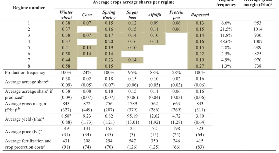
_{k it}x_, .

Farmers’ optimal crop acreage choices as given by equation (2a) can be derived for any production regime. It suffices to solve the maximization problem given in equations (3). For instance, eight acreage share subsystems are considered in our empirical application, one for each production regime present in the data. Of course, the functional form of the derived acreage choice function depends on the subset of crops produced in the considered regime. Assuming that crop k belongs to group g, we obtain:

13 _{The model used in our application is presented in the Online Appendix.} 14 _{We have we have}

( ),

s s g i i

17

(

)

(

(

)

)

(

)

(

)

1 ( ), 1 ( ), ( ) 1 ( ), , , _{( )} ( ), , , , _{( )} ( ), , , ( ) ( ) exp ( ) ( ) exp ( ) ( ) ( ) exp ( ) s s i g i s s i h i s s s s k g i k it k it _g g i it it k it s s h i it it h h j r j r s r j r a a a a

a

p

b

a

p

b

a

p

b

-Î Î Î - -=

-å

å å

(

_{g i it it})

)

)

(

, , ( ), , , , , ) expexp

(

(

( ),(( , , , , ( ), , , , ( ), , , ,

(

( ), , , , ( ), , , ,

(

( ), , , , ( ), , , , ( ), , , , ( ), , , , ((

(

( ), , , , ( , , ( , , ( , , ( , , ( , , ( , , _{( )} (( ) exp(( exp

(

( ((( , , _{( )} ( , , ( , , ( , , _{( )} ( , , ( , , _{( )( )( )( )g} ( , , ( , , ( , , ( , , ( , , ( , , ( , , ( , , ( , , ( , , ( , , ( , , ( , , ( , , ( , , ( , , ( , , ( , , ( , , _Î ( , , ( , , ( , , ( , , ( , , ( , , (

(

( ), , ,

)

)

) exp

(

_{( ),( ),}( _{,,,t ,,,it}) j r( )( )

(

(

_{( ),( ),( ),( ),( ),( ),( ),}(( _{,,,,, ,,,,,} ( ) h ( )( )h j h h hG h K K (10) and:

(

)

(

)

1 ( ), ( ) 1 ( ), , , ( ) ( ) ( ) ln ( ) exp ( ) s s i h i s s s it r i h h j r h i it it a a a a p b -Î Î

P =

å å

_{hhh ( )( )( )( )( )( )( )( )( )( )( )( )hhh} ( )) exp( )( ))( )( )) exp) expexpexp

(

(

(

(

(

(

_{( ),( ),( ),( ),( ),( ),( ),( ),( ),( ),( ),( ),( ),h i}( _,,,,,,,,,it- _,,,,,,,,,it)

)

)

G K . (11)

Parameter

a

is drives the land allocation to crop group acreages while parameters ( ),

s g i

a

drive the allocation of the crop group acreages to crop acreages.

3.3. Production regime choice model

Observing that the regime specific optimal acreage choice

s

_it

( )

r

necessarily belongs to regime

r in the MNL case considered here, the regime specific expected profit levels

P

_it

( )

r

can be used for defining a regime choice model based to the choice problem described in equation (4). Let define the regime fixed costs as

D r

_it

( )

=

d r

_i

( )

-

s

_i-1

e

_{r it,} . The farm specific parameters

d r

_i

( )

aim to capture the effects of unobserved factors affecting the regime fixed costs. The error terms

,

r it

e

aim to capture the effects of stochastic factors and define the regime choice model as a probabilistic discrete choice model, with:

{

1

}

,

arg max ( ) ( )

it r it i i r it

r = ÎR P r -d r +s-e . (12)

Scale parameter

s

_i determines the extent to which the regime expected profit levels (i.e. the

( )

( )

it

r

d r

i

P

-

terms) explain the production regime choice as regards to the effects of the

e

r it,

idiosyncratic terms. The higher

s

_i, the more the expected profit levels impact the observed regime choices.

Regime fixed costs

d r

_i

( )

can be specified in different ways. These costs are expected to increase with the number of crops. Transaction costs and labor requirements related to a production regime increase with the number of crops produced in that regime. Indeed, one way to specify

d r

_i

( )

is to consider a sum of fixed costs associated to each crop produced in the considered production regime, with _,

( ) ( ) c i _{k r} k i d r =

å

_ÎK+ b where , c k i

b

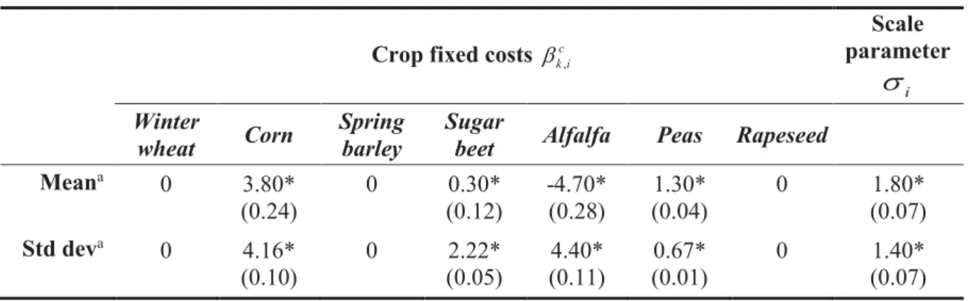
is the fixed costs related to crop k. Interestingly, this specification allows computing the fixed costs of regimes which are not observed in the data. This is of particular interest for simulation purposes. For example, changes in market conditions can lead farms to adopt new production regimes. This regime fixed cost specification is used in our empirical application.

18 Farmers may purchase inputs specific to different crops from the same supplier, implying savings in the related transaction costs. Moreover, different crops may generate work peak loads during the same periods, implying that can concentrate their workload (or that of their employees) during these periods if they wish so. In these cases, the regime fixed costs are sub-additive in the crop fixed costs. One way to deal with this pattern consists of directly specifying these fixed costs as famers specific constant terms on a regime per regime basis, with

d r

i

( )

=

d

r i,

(given that the fixed cost of a “benchmark regime” needs to be normalized). Of course, the costs corresponding to regimes that are not observed in the data can’t be recovered, thereby constraining the regime set that can be simulated to be equal to the one that is observed in the data.

3.4. Overall structure of the ERS-MEMC model

The ERS-MEMC model is composed of three main parts: a subsystem of yield supply and input demand equations (7), a set of per regime subsystems of acreage share equations (10) and a probabilistic regime choice model (12).

The set of dependent variables of this model contains the crop level production choices. These consist of the yield levels, input use levels and acreage shares of each crop that are produced by for farmer i in year t. These are collected in vector

(

y x s

_it+

,

_it+

, )

_it+ . Production regime

r

_it is the last dependent variable of the model.

The set of explanatory variables contains crop prices, variable input prices and the control variable vectors used in the crop yield supply, input demand and acreage share equations for all crops. These variable are collected in vector

z

_it, which defines the information set of the ERS-MEMC model.

The sole fixed parameters appearing in the model equations are the coefficients of the control variable coefficient vectors for all crops, which are collected in vector

δ

₀.

The considered ERS-MEMC model contains two main subsets of random components: a vector of random parameters and a vector of error terms.

Vector

γ

_i collects the farm specific parameters of the model, with

γ

_i

=

( , , )

β α

_{i i}

s

_i . This vector contains the potential yield parameters, the input requirement parameters, the cost function linear parameters and the crop fixed costs parameters for all crops. These random parameters are collected in vector

β

_i. It also contains the input use flexibility parameters for all crops and

19 the acreage choice flexibility parameters, which are collected in vector

α

_i. Finally,

γ

_i contains the scale parameter,

s

_i, of the regime choice model.

In the error term vector

ε

_it

=

(

ε

_ityx

, )

ε

_its , sub-vector

ε

_ityx collects the error terms error terms of crop yield supply and input demand equations for all crops while sub-vector

ε

s_it collects those of the acreage share equations. Finally, vector

e

_it collects the error terms of the regime choice model (i.e.,

e

r it, for

r

ÎR

).

4. ERS-MEMC model with regime specific fixed costs: estimation strategy

This section presents the main features of the estimation strategy adopted for estimating the ERS-MEMC model described above. As this model involve multiple endogenous regimes, considers numerous interrelated production choices and features random parameters, we impose parametric distributional assumptions on its random components (i.e. error terms and random parameters) that ensure its empirical tractability. We also impose simplifying assumptions regarding the dynamics of farmers’ choices and the multi-crop production technology. These assumptions are presented and discussed first. Then, we present how the main parameters of interest of our ERS-MEMC model are recovered from the data. Finally, we briefly describe our estimation strategy. More specifically, we present the main estimation issues that we face when estimating our random parameter ERS-MEMC model and the approaches chosen for overcoming these issues. A detailed description of our estimation procedure is provided in a dedicated Online Appendix. This procedure combines techniques found in the micro-econometrics and computational statistics literatures.

4.1. Main probabilistic assumptions

We assume that terms

( ,

ε e

_{is is}

)

,

γ

_i and

z

_it are independently distributed for any pair ( , )t s . This implies that the explanatory variables vector,

z

_it, is assumed to be (i) strictly exogenous with respect to the error term vectors and (ii) independent of the random parameters

γ

_i. This latter assumption, which is standard in random parameter models, defines

γ

_i as a term that captures heterogeneity effects not captured by control variables

z

_it.

We further assume that error term

( , )

ε e

_{it it} vectors are independently distributed across time. Combined with the fact that vector

z

_it doesn’t contain any lagged endogenous variable, this serial independence assumption implies that our MEMC model can be interpreted as a reduced

20 form model as regards the dynamic features of the modelled choices. Indeed, we hypothesize that random parameters

γ

_i capture the effects on farmers’ production choices and performances of the stable crop rotation schemes that these farmers rely on.15 Koutchadé et al. (2018) provide empirical results confirming this hypothesis with a sample of arable crop producers located in an area contiguous to the one considered in our application.

Finally, we assume that the error term vectors

ε

_ityx,

ε

s_it and

e

_it are independent. Relaxing this independence assumption for

ε

_its and

ε

_ityx is possible but significantly increases the estimation burden and Koutchadé et al. (2018), in a similar context, found that error terms

ε

_its and

ε

_ityx

were not significantly correlated.

4.2. Distributional assumptions

Random parameter vectors

γ

_i are assumed independent across farms. For sake of simplification, we assume here that these random parameter vectors are normally distributed, with

γ

_i

N

( ,

(μ

( ,

( ,

μ Ω

_{000000 000000}

)

. Various transformations of elements of

γ

_i actually allow for other distribution choices for these elements while keeping the multivariate structure of the probability distribution of

γ

_i (e.g., Stanfield et al., 1996). For example, considering log-transformations of

α

_i and

s

_i in

γ

_i implies that these random parameters, which are required to be positive, are jointly log-normality distributed. We used this log-transformation in the ESR-MEMC model used for our empirical application. Robustness checks demonstrated that other probability distribution choices have a limited impact on the main results.16

We make the usual assumptions stating that error term vectors

ε

_it are independent across farms (and years) and normally distributed, with

ε

_it

N

( ,

( ,

( ,

( ,

0 Ψ

₀₀₀

)

.17

Finally, we assume that the regime choice model error terms

e

_{r it,} are independent across regimes and distributed according to a type I extreme value distribution. This assumption implies that the considered regime choice model is a standard Multinomial Logit discrete choice

15 _{In that, we rely on well-known features of heterogeneous dynamic processes: those implying that empirically}

disentangling the effects of unobserved heterogeneity from those of unobserved persistent dynamic features is notably difficult. Accounting for dynamic features of multi-crop production technologies and of farmers’ choices is challenging, and largely beyond the scope of this article.

16 _{We tested specifications assuming that}

i

β is log-normally distributed and/or that α follows a bounded Johnson i

distribution (e.g., Stanfield et al, 1996).

17 _Matrix 0

Ψ is block-diagonal under the assumption stating that s it

ε and yx it

21 model conditionally on the scale parameter and on the regime specific expected profit levels and fixed costs. The corresponding conditional probability of the observed the regime choices is given by:

(

)

(

)

0

exp

(

( )

( ))

( |

, , ; )

exp

(

( )

( ))

s i it it i it it it it i i it i r

r

d r

P r

r

d r

s

s

Î

P

-=

P

-å

ε z γ δ

R . (13)

This probability is defined as a function of

( , , ; )

ε z γ δ

_its _{it i 0} because the vector of regime specific expected profit levels,

P

_it

( )

r

-

d r

_i

( )

for

r

ÎR

, is a function of all the terms contained in

0

( , , ; )

ε z γ δ

s_{it it i} , scale parameter

s

_i excepted.

4.3. Identification

We consider here identification of the probability distribution of main random parameters of interest: the production choice flexibility parameters and the parameters of the regime choice model.

Under the considered assumptions the probability distribution of farmers’ responses to economic incentives,

α

_i, are identified through two main channels. Identification of the probability distribution of the variable input use flexibility parameters,

a

_{k i}x_, for

k

ÎK

, mostly relies on the variations of the corresponding input to crop price ratios. Identification of the probability distribution of the acreage choice flexibility parameters,

a

_is and

a

_{( ),}s_{g i} for

g ÎG

, mainly relies on the variations of the expected crop return terms,

p

k it, for

k

ÎK

. Importantly,

the expected crop returns are defined as functions of random parameters (i.e.,

b

_{k i}y_, ,

b

_{k i}x_, and

,

x k i

a

for

k

ÎK

) that may be correlated with the acreage choice flexibility parameters. The “full” variance-covariance matrix of the joint probability distribution of the random parameters

i

γ

takes into account these potential correlations.

Scale parameter

s

_i, which is the random coefficient associated to the regime specific expected profit levels

P

_it

( )

r

in the regime choice model, is mainly identified by the variations in these variables. Crop fixed costs

b

_{k i}c_, are entailed in the regime fixed costs ( ) _{( )} ,

c

i _{k r} k i

d r =

å

_Î +

b

K .

Importantly, the fixed costs of the crops that are always produced cannot be identified because these crops are part of any regime present in the data. Therefore, the fixed costs of these crops are normalized at zero. The joint probability distribution of the identifiable crop fixed cost vector is mainly identified by the variations in the differences in the regime specific expected profit levels

P

_it

( )

r

across the production regimes. The potential correlations between, on the one

22 hand, the random parameters that are part of the expected profit levels and, on the other hand, the crop fixed costs and the scale parameter are taken into account in the distribution of

γ

_i.

4.4. Estimation issues and sketch of the estimation procedure

The considered ERS-MCEM model being fully parametric, we consider a Maximum Likelihood (ML) estimator for efficiently estimating its parameters. These parameters are collected in

θ

₀

=

( ,

δ Ψ μ Ω

_{0 0}

, ,

_{0 0}

)

. Contribution of farmer i to the likelihood function of the model corresponds to the probability density function (pdf) of her/his sequence of production choices conditional on the sequence of exogenous variables characterizing this choice sequence. Assuming that the considered pdf is parameterized by

η

, let function f u v η( | ; ) generically denotes the pdf of

u

_it conditional on

v

_it

=

v

at

u

_it

=

u

. And let function j( ;u Ω) denote the pdf of N( ,0 Ω)at u. Given the probabilistic assumptions defining the parametric version of the random parameter ERS-MEMC model, contribution of farmer i to the likelihood function at

_θ

is given by:

(

1

)

( )

T

(

,

, ,

|

, ; , )

(

; )

i _t

f

it it it

r

it it

j

d

+ + + =

=

_ò

Õ

-θ

y x s

z γ δ Ψ

γ μ Ω γ

( )

i

(

Õ

it i

ò

Õ

it i it i

ò

it i it i

))

it i

)

it i it i it . (14)

Likelihood function _ii

( )

( )

θ

can be obtained neither analytically nor numerically due to its integration over the probability distribution of the random parameters

γ

i .

Micro-econometricians generally solve this problem by integrating _ii

( )

( )

θ

via direct simulation methods for computing Simulated ML (SML) estimators of

θ

₀. Yet, implementing this approach is particularly challenging with ERS-MEMC models due to the dimension of parameter

θ

₀ and the complexity of the simulated version of the likelihood functions _ii

( )

( )

θ

))

. For instance, the ERS-MEMC model of our empirical application considers 22 production choices. It features 80 control variables, 37 random parameters and 20 error terms. Vector

θ

₀ contains 786 parameters while our dataset describes 40,192 observed production choices (16.5 per observation on average).

Integration of _ii

( )

( )

θ

over the random parameter distribution is thus the first estimation issue that we have to deal with. We compute the ML estimator of

θ

₀ by devising a Stochastic Approximate Expectation-Maximization (SAEM) algorithm. SAEM algorithms were proposed by Delyon et al. (1999) for computing ML estimators of models featuring continuous random parameters. These algorithms rely on simulation methods for integrating proxies of the sample log-likelihood of the considered model. They appear to use simulations more efficiently than