A benchmark problem to evaluate implementational issues for three-dimensional flows of incompressible fluids subject to slip boundary conditions

HAL Id: hal-03178710

https://hal.archives-ouvertes.fr/hal-03178710

Submitted on 24 Mar 2021

HAL is a multi-disciplinary open access

archive for the deposit and dissemination of

sci-entific research documents, whether they are

pub-lished or not. The documents may come from

teaching and research institutions in France or

abroad, or from public or private research centers.

L’archive ouverte pluridisciplinaire HAL, est

destinée au dépôt et à la diffusion de documents

scientifiques de niveau recherche, publiés ou non,

émanant des établissements d’enseignement et de

recherche français ou étrangers, des laboratoires

publics ou privés.

A benchmark problem to evaluate implementational

issues for three-dimensional flows of incompressible

fluids subject to slip boundary conditions

Radomir Chabiniok, Jaroslav Hron, Alena Jarolímová, Josef Málek,

Kumbakonam Rajagopal, Keshava Rajagopal, Helena Švihlová, Karel Tůma

To cite this version:

Radomir Chabiniok, Jaroslav Hron, Alena Jarolímová, Josef Málek, Kumbakonam Rajagopal, et

al.. A benchmark problem to evaluate implementational issues for three-dimensional flows of

in-compressible fluids subject to slip boundary conditions. Applications in Engineering Science, 2021, 6,

�10.1016/j.apples.2021.100038�. �hal-03178710�

ContentslistsavailableatScienceDirect

Applications

in

Engineering

Science

journalhomepage:www.elsevier.com/locate/apples

A

benchmark

problem

to

evaluate

implementational

issues

for

three-dimensional

flows

of

incompressible

fluids

subject

to

slip

boundary

conditions

R.

Chabiniok

_,

_J.

_Hron

_,

_A.

_Jarolímová

_,

_J.

_Málek

_,

_K.R.

_Rajagopal

_,

_K.

_Rajagopal

_,

H.

Š

vihlová

_,

_K.

_T

_ů

_ma

a Inria Saclay Ile-de-France, 1 Rue Honoré d’Estienne d’Orves, Palaiseau 91120, France b LMS, Ecole Polytechnique, CNRS, Institut Polytechnique de Paris, France

c Department of Mathematics, Faculty of Nuclear Sciences and Physical Engineering, Czech Technical University in Prague, Czech Republic d Department of Pediatrics, Division of Pediatric Cardiology, UT Southwestern Medical Center, Dallas, TX, United States

e Charles University, Faculty of Mathematics and Physics, Mathematical Institute, Sokolovská 83, Prague 186 75, Czech Republic f Texas A&M University, Department of Mechanical Engineering, College Station, TX 77843-3132, United States

g University of Houston College of Medicine and Houston Heart / HCA Houston Healthcare, Houston, Texas, United States

a

b

s

t

r

a

c

t

WeconsiderflowsofanincompressibleNavier–StokesfluidinatubulardomainwithNavier’sslipboundaryconditionimposedontheimpermeablewall.Wefocus onseveralimplementationalissuesassociatedwiththistypeofboundaryconditionswithintheframeworkofthestandardTaylor-Hoodmixedfiniteelementmethod andpresentthecomputationalresultsforflowsinatubulardomainoffinitelengthwithoneinletandoneoutlet.Inparticular,wepresentthedetailsregarding variantsoftheNitschemethodconcerningtheincorporationoftheimpermeabilityconditiononthewall.Wealsofindthatthemannerinwhichthenormalto theboundaryisnumericallyimplementedinfluencesthenatureofthecomputationalresults.Asabenchmark,wesetupsteadyflowsinatubeoffinitelengthand comparethecomputationalresultswiththeanalyticalsolutions.Finally,weidentifyvariousquantitiesofinterest,suchasthedissipation,wallshearstress,vorticity, pressuredrop,andprovidetheirprecisemathematicaldefinitions.Wedocumenthowwellthesequantitiesarecomputationallyapproximatedinthecaseofthe benchmark.

Althoughthegeometryofthebenchmarkissimple,thecorrectcomputationalresultsrequirecarefulselectionofnumericalmethodsandsurprisinglynon-trivial computationalresources.Ourgoalistotest,usingthesettingwithaknownanalyticalsolution,arobustcomputationaltoolthatwouldbesuitableforcomputations onrealcomplexgeometriesthathaverelevancetoproblemsinengineeringandmedicine.Themodelparametersinourcomputationsarechosenbasedonflowsin largearteries.

1. Introduction

Mostfluidsthatcanbe describedbytheNavier–Stokesmodelare assumedtomeettheno-slipboundarycondition,thatisadherenceof thefluidtotheboundary,inflowsthattakeplaceinpipes,channels, andothersimpledomainswhentheflowis reasonablyslow.The ap-plicationofthisparticularboundaryconditionisattributedtoStokes whois supposedtohaveadvocateditsuse.Itisnotreallyclearthat Stokesbelievedinitsgeneralvalidity.Heevenhaddoubtsconcerning itsaccuracyinpipesandchannels,asheremarked“DuBuatfoundby experimentthatwhenthemeanvelocityofwaterflowingthroughapipeis lessthanaboutoneinchinasecond,thewaterneartheinnersurfaceofthe pipeisatrest.Iftheseexperimentsmaybetrusted,theconditionstobe

sat-∗_{Correspondingauthor.Theorderoftheauthorsisalphabetical.}

E-mailaddresses: radomir.chabiniok@inria.fr(R.Chabiniok), jaroslav.hron@mff.cuni.cz(J.Hron), josef.malek@mff.cuni.cz(J.Málek), krajagopal@tamu.edu

(K.R.Rajagopal),keshava.rajagopal@gmail.com(K.Rajagopal),helena.svihlova@mff.cuni.cz(H.Švihlová),ktuma@karlin.mff.cuni.cz(K.Tůma).

isfiedinthecaseofsmallvelocitiesarethosewhichfirstoccurredtome,...” TheabovecommentishardlyarousingendorsementasStokesseemsto holdtheopinionthattheno-slipboundaryconditionisonlyappropriate forreasonablyslowflows.Moreover,Stokes(1845)alsoremarks“Ihave saidthatwhenthevelocityisnotverysmallthetangentialforcecalledinto actionbytheslidingofwaterovertheinnersurfaceofapipevariesnearly asthesquareofthevelocity”,statingquiteclearlythatslipistakingplace attheboundarywhentheflowsarenotsufficientlyslow.

Boundaryconditionsreflectthemutualinteractionbetweenthefluid flowinginsidethetubeandthematerialtheboundaryismadeof.For example,forflowsinbloodvessels,oneshouldtakeintoaccountthe propertiesofbloodaswellasoftheinnerpartofthevesselwall;the properboundaryconditionshoulddescribemutualinteractionbetween

https://doi.org/10.1016/j.apples.2021.100038

Received5December2020;Receivedinrevisedform22January2021;Accepted7February2021 Availableonline11February2021

thesematerials.Thisisdefinitelyaformidabletask.Formaterialssuch asblood(whichisacomplexmixtureofplasma1_{,redandwhiteblood} cells,platelets,lipo-proteins,andavarietyofcomplexions)andblood vessel(whichhasaverycomplexlayeredstructure)itisfarfromclear thattheno-slipboundaryconditionoughttohold,see(Rajagopaland Rajagopal,2020)formoredetails.

ExperimentsconcerningtheflowofbloodincapillariesbyBennett (1967)andBugliarelloandHayden(1963)report theslippingof red bloodcellsthatcomeintocontactwiththeboundary.InNubar(1967),

Nubar(1971),MisraandShit(2007),thepossibleconnectionofslippage onthewallandshearratedependentbloodviscositymeasuredinthe rheometerissuggested.Theaboveflowsarereasonablyslowflowsand eveninsuchflowscertaincomponentsofbloodseemtobeslippingat theboundary.Castingfurtherdoubtconcerningtheappropriatenessof theno-slipboundaryconditionisthefactthattheflowofbloodcanbe turbulentatsomelocationsinthecardiovascularsystemandfarfrom theslownesspresumedbyStokeswhentheno-slipboundarycondition isexperimentallyobserved.Thus,itwouldbeworthwhiletostudythe flowofamateriallikebloodbyassumingtheslipboundarycondition.

Numeroustypesofboundaryconditionsthatgobeyondtheno-slip boundarycondition wereproposed bytheearlypioneersinthefield of fluiddynamics (deCoulomb,1800; DuBuat,1786; Girard, 1813; Navier,1823;deProny,1804),andPoisson(1831). See(Netoetal., 2005)foramorerecentoverviewofexperimentalstudiesonboundary slipmeasurements.

Inthisstudy,wefocusonNavier’sslipboundarycondition(proposed byNavier,1823inagreementwithmoleculararguments)characterized bytheparameter𝜃 andinvolving,asthelimitingcases,no-slip bound-aryconditionatoneend(𝜃 =1)and(perfect)slipboundarycondition ontheotherend(𝜃 =0).Thisextendedclassofboundaryconditions, takingintoaccounttheslippingmechanismsofvariousdegree, repre-sentsthe most commonlyusedboundaryconditions imposedon the impermeablepartsoftheboundaryoftheflowdomain.Interestingly, itwasshown(see(Hronetal.,2008))thatforbothplaneand three-dimensionalPoiseuilleflowvaryingtheslipparameter𝜃 caninfluence theflowmoremarkedlythanthechangeoftheconstitutiveequationfor thefluid.

WeconsiderflowsofanincompressibleNavier–Stokesfluidina spe-cialthree-dimensionaldomain,namelyatubulardomainoffinitelength withoneinletandoneoutlettogetherwiththeabovedescribedclassof slipboundaryconditionsimposedontheimpermeablewall.Thereason forchoosingthisspecialgeometricalsetupistwofold.First,knowingthe analyticalsolutionsforsteadyflowssubjecttodifferentslippageatthe wallofcylinder,weareabletosetabenchmarkthatcanserveasabasic testforvariousnumericalmethodsandtheirimplementations.Second, thisgeometricalsettingcanbeviewedasaverysimplified,yet reason-ableapproximationofflowsinalargevessels,applicableforinstance wheninvestigating/assessingflowthroughaorticvalve(nativeorits re-placement),orapathologicallynarrowedsegmentoflargeartery(e.g. coarctationofaortaorpulmonaryarterystenosis).

Next,wepresentenergeticconsiderationsthatmightprovidesupport forthechoiceofboundaryconditionsthatweenforceatarigid bound-aryandattheoutletandprovidethefunctionspacesinwhichtheweak formulationsoftheproblemisformulated.Theseformulationsdiffer de-pendingonhowtheincompressibilityconstraintandtheimpermeability conditionareincorporated.Inparticular,wepresentthedetails regard-ingvariantsoftheNitschemethod(Nitsche,1971)concerning(inthis study)theincorporationoftheimpermeabilityconditiononthewall. WeprovidealiteratureoverviewconcerningtheNitschemethodatthe endofSection3.

Then,wefocusonseveralissuesassociatedwiththeimplementation ofthistypeofboundaryconditionswithintheframeworkofthe

stan-1 _{PlasmaisoftentimesdescribedbyaNavier–Stokesfluidwhileflowingin}

largebloodvessels.

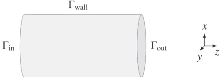
Fig.1. Computationaldomainandthepartsoftheboundary.

dardTaylor-Hoodfiniteelements.Wediscusshowthemannerinwhich thenormaltotheboundaryisnumericallyimplementedinfluencesthe natureofthecomputationalresults.Wealsoidentifyvariousquantities ofinterest,suchasthedissipation,pressuredrop,vorticity,wallshear stress,andprovidetheirprecisemathematicaldefinitions.Theobjective istodocumenthowwellthesequantitiesarecomputationally approxi-matedinthecaseoftheproposedbenchmark.

Wewouldliketoemphasizethatalthoughthegeometryofthe bench-markissimple,thecorrectcomputationalresultsrequireacareful selec-tionofnumericalmethodsandnon-trivialcomputationalresources.Our goalistotest,usingthesettingwithaknownanalyticalsolution,a ro-bustcomputationaltoolthatwouldbesuitableforcomputationsonreal complexgeometriesthathaverelevancetoproblemsinengineeringand medicine.Themodelparametersinourcomputationsarechosenbased onflowsinlargearteries;thiscorrespondstoflowsatReynoldsnumber ofapproximately1050.

Thestructureofthepaperisthefollowing.InSection2.1,we formu-latetheproblemdescribingunsteadyflowsofincompressibleNavier– Stokesfluidinthree-dimensionaltubewithNavier’sslipboundary con-ditionontheimpermeablewall,agivenvelocityattheinletandspecial boundaryconditionsattheoutletthattakesintoaccountthegiven nor-malstress(i.e.thepressure)aswellasthecontrol(boundedness)ofthe energyofthewholesystem.Theenergyconsiderationsalsoleadtothe choiceofthefunctionspacesinwhichwestatetheweakformulation oftheproblem.InSection3,wetakeaslightlydifferentviewpointwith regardtotheweakformulationoftheproblemandwediscusstwo vari-antsoftheNitschemethodthatareusedtonumericallyincorporate,in aweaksense,theimpermeabilitycondition.Section4providesabrief descriptionofthenumericaldiscretizationofweakformulations con-nectedwiththeNitschemethod.Theemphasisisdevotedtothewayin whichthenormalvectorisimplemented.InSection5,thebenchmark withknownanalyticalsolutionunderthesimplifyingassumptionofthe simpleshearflowisformulated.Wealsodefinetwoformsofmechanical dissipationofthesystemandpresentitsconnectiontothekineticenergy andthepressuredropalongthelengthofthetube.Pressuredropisoften usedinlieuofthedissipationrateincaseswheretherealdissipationis unknown.ThisisclarifiedinSection5.2.Section6bringstogetherall theresultsconnectedwithournumericalapproachandcomputational toolsandcomparesthemwiththeanalytical(benchmark)solution.We alsocomparetheefficiencyofthevariantsoftheNitschemethod.The concludingSection7summarizesthemainresultsthathavebeen estab-lished.

2. Definitionoftheproblemandenergyconsideration

2.1. Formulationoftheinitial-boundary-valueproblem

WeconsidertheflowofanincompressibleNavier–Stokesfluidover timeinterval𝑇,inathree-dimensionaltube ofthefinitelength rep-resentingabounded,openandconnectedsetΩ⊂ 𝐑3_{,seeFig.1. The}

unsteady flows of suchfluids described in termsof the velocity𝐯= (𝑣1,𝑣2,𝑣3)∶(0,𝑇)× Ω→ 𝐑3 andthe mean normalstress −𝑝∶(0,𝑇)×

followingsetofequations: div𝐯=0 in(0,𝑇)× Ω, (1) 𝜌∗𝜕𝐯_𝜕𝑡 +𝜌∗(∇𝐯)𝐯=div𝕋 in(0,𝑇)× Ω, (2) 𝕋=−𝑝𝕀+𝜇∗ ( ∇𝐯+∇𝐯𝑇) in(0,𝑇)× Ω, (3) where𝕋istheCauchystressand𝜌∗>0,𝜇∗>0aregivenconstants:the

densityandthedynamicviscosity.Wealsousethenotation

[(∇𝐯)𝐯]_𝑖= 3 ∑ 𝑘=1 𝜕𝑣𝑖 𝜕𝑥𝑘𝑣𝑘= 3 ∑ 𝑘=1 𝜕 𝜕𝑥𝑘(𝑣𝑘𝑣𝑖)=∶[div(𝐯⊗ 𝐯)], 𝑖=1,2,3, wheretheincompressibilityconstraint(1)hasbeenincorporated. Fur-thermore,foranymatrix𝔸,thesymbol𝔸𝑇 _{denotesitstranspose.}

Theboundary𝜕Ω ofthetubulardomainΩconsistsofthree non-overlappingpartsΓin,ΓoutandΓwallandweimposethefollowinginitial

andboundaryconditionsinvolvingthreegivenfunctions:𝐯0∶Ω→ 𝐑3,

𝐯in:[0,𝑇]× Γin→ 𝐑3and𝑃:[0,𝑇]→ 𝐑: 𝐯(0,⋅)=𝐯0 inΩ, (4) 𝐯=𝐯in on(0,𝑇)× Γin, (5) 𝕋𝐧=−𝑃(𝑡)𝐧+1 2𝜌∗(𝐯⋅ 𝐧)−𝐯 on(0,𝑇)× Γout, (6) 𝐯⋅ 𝐧=0 and 𝜃𝐯𝜏+𝛾∗(1−𝜃)(𝕋𝐧)𝜏=𝟎 on(0,𝑇)× Γwall. (7)

Here𝜃 ∈ [0,1],𝛾∗∈ (0,∞)and𝐧isaunitnormalvectorattheboundary.

Furthermore,for𝑥∈𝐑weset𝑥+∶=max{0,𝑥}and𝑥−∶=min{0,𝑥},i.e.

𝑥=𝑥++𝑥−,andforanarbitraryvector𝐳,𝐳𝐧∶=(𝐳⋅ 𝐧)𝐧isthenormal

componentof𝐳 and𝐳𝜏∶=𝐳−𝐳𝐧 istheprojectionof 𝐳 tothetangent

plane.

Notethatinsteadof(6)wecouldimposethecondition

𝐯𝜏=𝟎 and 𝕋𝐧⋅ 𝐧=−𝑃(𝑡)+1 2𝜌∗(𝐯⋅ 𝐧)

2

− on(0,𝑇)× Γout. (8)

Bytakingthe scalarproductof (6)with𝐧,we observethat(6)and

(8)givetheidenticaldescriptioninthenormaldirection.Ontheother hand,byprojecting(6)intothetangentplane,weobtain1

2𝜌∗(𝐯⋅ 𝐧)−𝐯𝜏=

(𝕋𝐧)_𝜏,whichisdifferentthanthefirstconditionin(8).Thecondition

(8)ismoreappropriatetothesituationswherethevelocityfieldatthe outflowis unidirectional(whichis,infact,thecaseoftheanalytical solutionusedinSection5).Althoughtheboundaryconditions(8)are differentthanthosestatedin(6),inthefewcomputationaltestsmade sofarwehavenotobservedanysignificantdifference.Thisiswhythe conditions(8)arenotdiscussedanymorebelowandweconsidermerely

(6)atΓoutinwhatfollows.

Theboundaryconditions(6),(7)andthefunctionspacesfortheweak formulationareinkeepingwithbasicenergyestimatesthatcanbe es-tablishedfortheproblem(1)–(7),seebelow.Wewishtoremarkthat thepresenceoftheterm1₂𝜌∗(𝐯⋅ 𝐧)−𝐯intheoutflowboundarycondition (6)seems tobe essentialnotonlyforobtainingtheenergyestimates (seebelow) butalsofortherobustnessandstabilityofthenumerical methods.

2.2. Energybalanceandenergyestimates

Forclarity,weproceedintwosteps.First,wesimplifythesettingby assumingthat

𝐯in=𝟎. (9)

Ageneralinflowfunctionwillbeconsideredlater.

Toobtaintheenergyidentity,assuming(9),weformthescalar prod-uctof(2)with𝐯,use(1)andarriveat

𝜕 𝜕𝑡 ( 𝜌∗|𝐯| 2 2 ) +div ( 𝜌∗|𝐯| 2 2 𝐯−𝕋𝐯 ) +𝕋⋅ 𝔻(𝐯)=0, (10)

where𝔻(𝐯)isthesymmetric partof thevelocitygradientdefined as

1 2

(

∇𝐯+∇𝐯𝑇).ThenweintegratethisequationoverΩ,applytheGauss theorem, usetheimpermeabilityconditionon Γwall andthe

homoge-neousDirichletconditiononΓinandconcludethat

d d𝑡∫Ω𝜌∗ |𝐯|2 2 d𝑥+∫Ω𝕋⋅ 𝔻 (𝐯)d𝑥+ ∫Γ_out𝜌∗ |𝐯|2 2 𝐯⋅ 𝐧d𝑆 + ∫Γ_wall∪Γ_out −𝕋𝐯⋅ 𝐧d𝑆=0. (11)

Duetothesymmetryof𝕋,wehave𝕋𝐯⋅ 𝐧=𝕋𝐧⋅ 𝐯,andbydecomposing thevectors𝕋𝐧and𝐯intotheirnormalcomponentandprojectioninto thetangentplaneandusingtheimpermeabilityconditiononΓwallwe

concludefrom(11)that

d d𝑡∫Ω𝜌∗ |𝐯|2 2 d𝑥+∫Ω𝕋⋅ 𝔻 (𝐯)d𝑥+ ∫Γwall −(𝕋𝐧)_𝜏⋅ 𝐯_𝜏d𝑆 + ∫Γout 𝜌∗|𝐯| 2 2 (𝐯⋅ 𝐧)+d𝑆=∫Γout ( 𝕋𝐧⋅ 𝐯−𝜌∗|𝐯| 2 2 (𝐯⋅ 𝐧)− ) d𝑆. (12) Thisstructureisconsistentwiththeboundaryconditions(6)and(7)to beconsideredinthisstudy.Takingintoaccounttheincompressibility condition(1),(12)canbeexpressedas(seeBraackandMucha,2014)

d d𝑡∫Ω𝜌∗ |𝐯|2 2 d𝑥+∫Ω𝕋⋅ 𝔻 (𝐯)d𝑥+ ∫Γ_wall −(𝕋𝐧)_𝜏⋅ 𝐯_𝜏d𝑆 + ∫Γout 𝜌∗|𝐯| 2 2 (𝐯⋅ 𝐧)+d𝑆 =− ∫Γout 𝑃(𝑡)𝐯⋅ 𝐧d𝑆=−𝑃(𝑡) ∫_𝜕Ω𝐯⋅ 𝐧d𝑆=−𝑃(𝑡)∫Ω div𝐯d𝑥=0. (13)

Asthefluidisincompressiblethereisanindeterminateparttothestress thatisspherical.Setting−𝑝∶=1₃(𝕋11+𝕋22+𝕋33),i.e.themeannormal

stress, wehave𝕋 =−𝑝𝕀+𝕋_𝑑,where𝕋𝑑∶=𝕋−13(𝕋11+𝕋22+𝕋33)𝕀.

Ne-glecting, forsimplicity,thelast (non-negative)termon theleft-hand sideof(13)andapplyingtheintegrationw.r.t.timeover(0,𝑡),𝑡∈ (0,𝑇], weget ∫Ω𝜌∗ |𝐯(𝑡,𝑥)|2 2 d𝑥+∫ 𝑡 0 ∫Ω𝕋𝑑⋅ 𝔻 (𝐯)d𝑥d𝜏 + ∫ 𝑡 0 ∫Γwall −(𝕋𝐧)_𝜏⋅ 𝐯_𝜏d𝑆d𝜏 ≤_∫ Ω𝜌∗ |𝐯0(𝑥)|2 2 d𝑥. (14)

Theaboveequationstatesthatthetotalkineticenergyattime𝑡andthe sumofthedissipatedenergyduetointernalfrictioninthefluid consid-eredover(0,𝑡)× Ωandthedissipatedenergyduetofrictioncausedby interactionofthefluidwiththeinnerpartoftheboundaryiscontrolled (bounded)bytheinitialkineticenergy.Inordertobeconsistentwith thesecondlawofthermodynamics,thetotaldissipatedenergyhastobe non-negative.This isforexampleautomaticallyfulfilled byrequiring that

𝕋𝑑=2𝜇∗𝔻(𝐯) on(0,𝑇)× Ω, (15)

−(𝕋𝐧)_𝜏= 1

̃𝛾∗𝐯𝜏

on(0,𝑇)× Γwall, (16)

where𝜇∗and̃𝛾∗arepositiveconstantsrepresentingthedynamic

viscos-ityandthefrictioncoefficient,respectively.WenotethatEqs.(15)and

(16)areconstitutiverelationsandarelinear.Inordertoincorporatea parameterthatmeasuresthevariousdegreesofslippageandincludes

alsono-slip(𝐯𝜏=𝟎)and(perfect)slip((𝕋𝐧)𝜏=𝟎)boundaryconditions weintroducetheequation

𝜃𝐯𝜏+𝛾∗(1−𝜃)(𝕋𝐧)𝜏=𝟎 on(0,𝑇)× Γwall, (17)

where0≤𝜃 ≤1insteadof(16).Toconclude,uponinserting(15)and

(17)into(14),weobtainthefollowingenergyinequalityfor𝜃 ∈ (0,1): ∫Ω𝜌∗ |𝐯(𝑡,𝑥)|2 2 d𝑥+2𝜇∗∫ 𝑡 0 ∫Ω|𝔻 (𝐯)|2_d𝑥d𝜏 + 𝜃 𝛾∗(1−𝜃)∫ 𝑡 0 ∫Γwall |𝐯𝜏|2d𝑆d𝜏 ≤ ∫Ω𝜌∗ |𝐯0(𝑥)|2 2 d𝑥. (18)

For𝜃 =0or𝜃 =1theenergyinequalitytakesasimplerform,namely ∫Ω𝜌∗ |𝐯(𝑡,𝑥)|2 2 d𝑥+2𝜇∗∫ 𝑡 0 ∫Ω|𝔻 (𝐯)|2d𝑥d𝜏 ≤ ∫Ω𝜌∗ |𝐯0(𝑥)|2 2 d𝑥. (19) Next,weconsiderthecompleteformulation(1)–(7),i.e.withgeneral inflowvelocity𝐯in.Weassumetheexistenceofanextension𝐯∗inof𝐯in,i.e.

werequirethatthereexistsacontinuousfunction𝐯∗

in∶(0,𝑇)× Ω→ 𝐑 3_,

ΩbeingtheclosureofΩ,suchthat div𝐯∗_in=0 in (0,𝑇)× Ω, 𝐯∗ in=𝐯in onΓin, 𝐯∗ in⋅ 𝐧=0 on Γwall, 𝐯∗ in=𝟎 on Γout, 𝜕𝐯∗ in 𝜕𝑡 ∈𝐿2((0,𝑇)× Ω)3 and∇𝐯∗in∈𝐿 ∞_{((0,𝑇)× Ω)}3×3_. (20)

Toobtaintheenergyequality,wemodifytheaboveprocedureandform thescalarproductof(2)with𝐯−𝐯∗_in.Doingso,weobtain

𝜕 𝜕𝑡 ( 𝜌∗ |𝐯−𝐯∗_in|2 2 ) +div ( 𝜌∗ |𝐯−𝐯∗_in|2 2 𝐯 ) −div(𝕋(𝐯−𝐯∗_in))+𝕋⋅ 𝔻(𝐯−𝐯∗_in) =−𝜌∗ 𝜕𝐯∗ in 𝜕𝑡 ⋅ (𝐯−𝐯∗in)−𝜌∗𝑣𝑘 𝜕𝐯∗ in 𝜕𝑥𝑘 ⋅ (𝐯−𝐯 ∗ in) =−𝜌∗ 𝜕𝐯∗ in 𝜕𝑡 ⋅ (𝐯−𝐯∗in)−𝜌∗(𝐯−𝐯∗in)⊗ (𝐯−𝐯 ∗ in)⋅ ∇𝐯 ∗ in −𝜌∗((𝐯−𝐯∗in)⊗ 𝐯 ∗ in)⋅ ∇𝐯 ∗ in =−𝜌∗ 𝜕𝐯∗ in 𝜕𝑡 ⋅ (𝐯−𝐯∗in)−𝜌∗(𝐯−𝐯∗in)⊗ (𝐯−𝐯 ∗ in)⋅ ∇𝐯 ∗ in +𝜌∗(𝐯∗in⊗ 𝐯 ∗ in)⋅ 𝔻(𝐯−𝐯 ∗ in)−div ( 𝜌∗(𝐯∗in⋅ (𝐯−𝐯 ∗ in))𝐯 ∗ in ) . (21)

ThenweintegratethisequationoverΩanduseGauss’stheorem.Using alsothepropertiesof𝐯∗

ingivenin(20),weobtain d d𝑡∫Ω𝜌∗ |𝐯−𝐯∗ in| 2 2 d𝑥+∫Ω𝕋⋅ 𝔻 (𝐯−𝐯∗_in)d𝑥+ ∫Γwall −(𝕋𝐧)_𝜏⋅ (𝐯_𝜏−(𝐯∗_in)_𝜏)d𝑆 + ∫Γout 𝜌∗|𝐯| 2 2 (𝐯⋅ 𝐧)+d𝑆 =− ∫Ω 𝜌∗ 𝜕𝐯∗ in 𝜕𝑡 ⋅ (𝐯−𝐯∗in)d𝑥−_∫ Ω 𝜌∗(𝐯−𝐯∗in)⊗ (𝐯−𝐯 ∗ in)⋅ ∇𝐯 ∗ ind𝑥 + ∫Ω𝜌∗ (𝐯∗_in⊗ 𝐯∗_in)⋅ 𝔻(𝐯−𝐯∗_in)d𝑥−𝑃(𝑡) ∫Γout 𝐯⋅ 𝐧d𝑆. (22) Uponinsertingtheconstitutiveequations(15)and(17)(noticingthat theboundaryintegralonΓwallvanishesfor𝜃 =0and𝜃 =1priorto

in-serting)andneglectingthelast(non-negative)termontheright-hand sideof(22)wearriveat d d𝑡∫Ω𝜌∗ |𝐯−𝐯∗ in| 2 2 d𝑥+2𝜇∗∫Ω|𝔻 (𝐯−𝐯∗_in)|2d𝑥 + 𝜃 𝛾∗(1−𝜃) { ∫Γwall |𝐯𝜏|2d𝑆−_∫ Γwall 𝐯𝜏⋅ (𝐯∗in)𝜏d𝑆 } ≤− ∫Ω𝜌∗ (𝐯−𝐯∗ in)⊗ (𝐯−𝐯 ∗ in)⋅ ∇𝐯 ∗ ind𝑥+_∫ Ω𝜌∗ (𝐯∗ in⊗ 𝐯 ∗ in)⋅ 𝔻(𝐯−𝐯 ∗ in)d𝑥 − ∫Ω𝜌∗ 𝜕𝐯∗ in 𝜕𝑡 ⋅ (𝐯−𝐯∗in)d𝑥+𝑃(𝑡)_∫ Γin 𝐯⋅ 𝐧d𝑆 −2𝜇∗_∫ Ω 𝔻(𝐯∗ in)⋅ 𝔻(𝐯−𝐯 ∗ in)d𝑥, (23)

wherethelast termhasbeenaddedtotheleft-handside.Next, inte-grating(23)w.r.t.timeandusingthestandardnotationforthenorms intheLebesguespaces(𝐿𝑝(Ω),‖ ⋅ ‖_𝑝)for1≤𝑝≤∞,andusingalsothe standardCauchy–Schwartz,YoungandHölderinequalities,weobtain

1 2𝜌∗‖(𝐯−𝐯 ∗ in)(𝑡,⋅)‖ 2 2+2𝜇∗_∫ 𝑡 0 ‖𝔻 (𝐯−𝐯∗_in)‖2₂d𝑠 + 𝜃 𝛾∗(1−𝜃)∫ 𝑡 0 ∫Γwall |𝐯𝜏|2_d𝑆d𝑠 ≤ 1 2𝜌∗‖𝐯0−𝐯 ∗ in(0,⋅)‖ 2 2+ 3𝜇∗ 2 ∫ 𝑡 0 ‖𝔻(𝐯−𝐯∗ in)‖ 2 2d𝑠 +𝐶(𝐯∗_in)𝜌∗_∫ 𝑡 0 ‖𝐯 −𝐯∗_in‖2₂d𝑠+𝑃(𝑡) ∫ 𝑡 0 ∫Γin 𝐯in⋅ 𝐧d𝑆d𝑠 +1 2 𝜃 𝛾∗(1−𝜃)∫ 𝑡 0 ∫Γwall (|𝐯_𝜏|2+|(𝐯∗_in)𝜏|2)d𝑆d𝑠+𝐶(𝐯∗_in), (24)

where the constant 𝐶(𝐯∗

in) depends on 𝜌∗, 𝜇∗, ∫0𝑇‖‖‖‖ 𝜕𝐯∗ in 𝜕𝑡 ‖‖‖‖ 2 2 d𝑠, ∫0𝑇‖𝔻(𝐯 ∗ in)‖ 2

2d𝑠 and sup𝑡∈(0,𝑇 )‖∇𝐯∗in‖∞ and is finite due to the

as-sumptionson𝐯∗

instatedin(20).

Finally,movingthesecondtermfromtheright-handsidetotheleft andapplyingtheGronwalllemmaweconcludethat

𝜌∗ sup 𝑡∈[0,𝑇 ]‖(𝐯−𝐯 ∗ in)(𝑡,⋅)‖ 2 2+𝜇∗_∫ 𝑇 0 ‖𝔻 (𝐯−𝐯∗_in)‖2₂d𝑡 + 𝜃 𝛾∗(1−𝜃)∫ 𝑇 0 ∫Γwall |𝐯𝜏|2d𝑆d𝑡 ≤𝐶(𝑇,‖𝐯0−𝐯∗in(0,⋅)‖ 2 2,𝐶(𝐯 ∗ in) ) <∞. (25)

2.3. Definitionofweaksolutiontotheproblem(1)–(7)

Let 𝑊1,2 div, bc∶= { 𝜙𝜙𝜙 ∈ 𝑊1,2_(Ω)3_{; div𝜙𝜙𝜙 =0,𝜙𝜙𝜙 =𝟎onΓ} in,𝜙𝜙𝜙 ⋅ 𝐧=0onΓwall } .

Motivatedbytheaboveenergyestimates,bytheconceptofLeray-Hopf weaksolutionfortheNavier–Stokesequationswithno-slipboundary conditions,andbytheresultsconcerningthe𝐿𝑝_{-maximalregularityfor} theevolutionaryStokessystem,we saythatacouple(𝐯,𝑝)is aweak solutionto(1)–(7)providedthat

𝐯−𝐯∗ in ∈ 𝐿 2_(0,𝑇;𝑊1,2 div, bc)∩𝐶𝑤𝑒𝑎𝑘([0,𝑇];𝐿 2_(Ω)3_), 𝜕𝐯 𝜕𝑡 ∈ 𝐿5∕4(0,𝑇;𝐿5∕4(Ω)), ₍₂₆₎ 𝑝∈ 𝐿5∕4_(0,𝑇;𝑊1,5∕4_(Ω)), lim 𝑡→0+‖𝐯(𝑡,⋅)−𝐯0‖2→ 0, and ∫Ω 𝜌∗𝜕𝐯_𝜕𝑡⋅ 𝜙𝜙𝜙 d𝑥+_∫ Ω 𝜌∗(∇𝐯)𝐯⋅ 𝜙𝜙𝜙 d𝑥+2𝜇∗_∫ Ω 𝔻(𝐯)⋅ 𝔻(𝜙𝜙𝜙)d𝑥 + 𝜃 𝛾∗(1−𝜃)∫Γ_wall𝐯𝜏⋅ 𝜙𝜙𝜙𝛕 d𝑆 =−𝑃(𝑡) ∫Γout 𝜙𝜙𝜙 ⋅ 𝐧d𝑆+ ∫Γout 𝜌∗ 2(𝐯⋅ 𝐧)−𝐯⋅ 𝜙𝜙𝜙 d𝑆 validforall𝜙𝜙𝜙 ∈ 𝑊1,2

Alternatively,insteadof(27),onecanconsider ∫Ω𝜌∗ 𝜕𝐯 𝜕𝑡⋅ 𝜙𝜙𝜙 d𝑥−∫Ω𝜌∗ (𝐯⊗ 𝐯)⋅ ∇𝜙𝜙𝜙 d𝑥+2𝜇∗_∫ Ω𝔻 (𝐯)⋅ 𝔻(𝜙𝜙𝜙)d𝑥 + 𝜃 𝛾∗(1−𝜃)∫Γwall 𝐯𝜏⋅ 𝜙𝜙𝜙𝛕d𝑆+_∫ Γout 𝜌∗(𝐯⋅ 𝐧)𝐯⋅ 𝜙𝜙𝜙 d𝑆 =−𝑃(𝑡) ∫Γout 𝜙𝜙𝜙 ⋅ 𝐧d𝑆+ ∫Γout 𝜌∗ 2(𝐯⋅ 𝐧)−𝐯⋅ 𝜙𝜙𝜙 d𝑆 validforall𝜙𝜙𝜙 ∈ 𝑊1,2

div, bcanda.a.𝑡∈ (0,𝑇). (28)

3. TheNitschemethod

Inthissectionwemodifytheweakformulation(27)sothatthe in-compressibilityconstraint(1)andtheimpermeabilitycondition(7)1on

thewallaretreatedinamannersuitablefornumericalimplementation. Thus,thefunctionspace𝑊1,2

div, bc introducedintheprevioussectionis modifiedinsuchawaythatittakesintoaccountonlytheinflow bound-arycondition,i.e.insteadofusing𝑊1,2

div, bcthevelocity𝐯isnowsought inthespace𝑉 suchthat

𝑉 ∶={𝐯∈𝑊1,2(Ω)3,𝐯=𝟎onΓin}. (29)

Thenweproceedasfollows.First,theincompressibilityconstraint

(1)ismultipliedbythetestfunction𝑞∈𝐿2_{(Ω)andintegratedoverΩ.}

Then,thebalanceoflinearmomentum(2)ismultipliedbythetest func-tion𝜙𝜙𝜙 ∈ 𝑉 integratedoverΩfollowedbytheintegrationbypartswith respecttotheterminvolving−div𝕋.Next,theimpermeability condi-tionwrittenwithrespecttotheform−𝐯𝐯𝐯_𝐧=𝟎onΓwallismultipliedby

thetestfunction𝜓𝜓𝜓∈𝐿2_(Γ

wall)3 andintegratedoverΓwall. Finally,we

sumtheestablishedidentitiesandobtain

∫Ω ( 𝜌∗𝜕𝐯_𝜕𝑡+𝜌∗(∇𝐯)𝐯 ) ⋅ 𝜙𝜙𝜙 d𝑥+ ∫Ω𝕋 (𝐯,𝑝)⋅ ∇𝜙𝜙𝜙 d𝑥+ ∫Ω (div𝐯)𝑞d𝑥 + ∫Γwall 𝜃 𝛾∗(1−𝜃)𝐯𝜏⋅ 𝜙𝜙𝜙𝜏 d𝑆− ∫Γwall (𝕋(𝐯,𝑝)𝐧)_𝐧⋅ 𝜙𝜙𝜙_𝐧d𝑆− ∫Γwall 𝐯𝐧⋅ 𝜓𝜓𝜓d𝑆 − ∫Γout ( −𝑃(𝑡)𝐧+1 2𝜌∗(𝐯⋅ 𝐧)−𝐯 ) ⋅ 𝜙𝜙𝜙 d𝑆=0

forall(𝑞,𝜙𝜙𝜙,𝜓𝜓𝜓)∈ (𝐿2(Ω)×𝑉×𝐿2(Γwall)3), (30)

whereweusethenotation𝕋(𝜙𝜙𝜙,𝑞)∶=−𝑞𝕀+2𝜇𝔻(𝜙𝜙𝜙)andwherewealso usedtheobservationthat

∫_𝜕Ω𝕋𝐧⋅ 𝜙𝜙𝜙 d𝑆=∫Γout ( −𝑃(𝑡)𝐧+1 2𝜌∗(𝐯⋅ 𝐧)−𝐯 ) ⋅ 𝜙𝜙𝜙 d𝑆 − ∫Γwall 𝜃 𝛾∗(1−𝜃)𝐯𝜏⋅ 𝜙𝜙𝜙𝜏 d𝑆+ ∫Γwall (𝕋𝐧)_𝐧⋅ 𝜙𝜙𝜙_𝐧d𝑆. (31)

Theformulation(30)requiresspecialtestfunctions𝜓𝜓𝜓 definedonthe boundaryΓwallwhichoneneedstoenlargetheproblem.Itistempting

toreplacethisnewtestfunctionbyacombinationof𝑞 and𝜙𝜙𝜙,whichis possibleas𝜓𝜓𝜓actson𝐯whichisalreadytheunknown.

Inspiredbythestructureofthelast twotermsin themiddleline of(30)weusethetestfunction𝜓𝜓𝜓=(𝕋(𝜙𝜙𝜙,𝑞)𝐧)_𝐧andobtaintheoriginal Nitschemethod.Nitsche(1971)showedthatsuchaformulationisnot stable,butwhenoneaddsthestabilizationterm

𝛽 ℎ∫Γwall

𝐯𝐧⋅ 𝜙𝜙𝜙𝐧d𝑆, 𝛽 >0 (32)

theweakformbecomesstableforsufficientlylargeparameter𝛽 >0.The localsizeofmeshedgeisdenotedbyℎ.Sincetheextraterm−∫_Γ

wall𝐯𝐧⋅

(𝕋(𝜙𝜙𝜙,𝑞)𝐧)_𝐧d𝑆 hasthesamesign astheterm−∫_Γ

wall(𝕋(𝐯,𝑝)𝐧)𝐧⋅ 𝜙𝜙𝜙𝐧d𝑆,

thismethodiscalledthesymmetricNitschemethod.Theweakformulation toourproblemusingthesymmetricNitschemethodthenreads:

Find(𝐯−𝐯∗_in,𝑝)∈𝐿∞(0,𝑇;𝐿2(Ω)3)∩𝐿2(0,𝑇;𝑉)×𝐿5∕4(0,𝑇;𝐿2(Ω)) suchthat ∫Ω ( 𝜌∗𝜕𝐯_𝜕𝑡 +𝜌∗(∇𝐯)𝐯 ) ⋅ 𝜙𝜙𝜙 d𝑥+2𝜇∗_∫ Ω𝔻 (𝐯)⋅ 𝔻(𝜙𝜙𝜙)d𝑥 − ∫Ω𝑝 (div𝜙𝜙𝜙)d𝑥+ ∫Ω (div𝐯)𝑞d𝑥− ∫Γout ( −𝑃(𝑡)𝐧+1 2𝜌∗(𝐯⋅ 𝐧)−𝐯 ) ⋅ 𝜙𝜙𝜙 d𝑆 + ∫Γwall 𝜃 𝛾∗(1−𝜃)𝐯𝜏⋅ 𝜙𝜙𝜙𝜏 d𝑆− ∫Γwall (𝕋(𝐯,𝑝)𝐧)_𝐧⋅ 𝜙𝜙𝜙_𝐧d𝑆 − ∫Γwall 𝐯𝐧⋅ (𝕋(𝜙𝜙𝜙,𝑞)𝐧)_𝐧d𝑆+𝛽 ℎ∫Γwall 𝐯𝐧⋅ 𝜙𝜙𝜙𝐧d𝑆=0

forall (𝝓,𝑞)∈𝑉×𝐿2(Ω)anda.a.𝑡>0. (33)

Themaindisadvantageofaddingstabilization(32)isthatthe pa-rameter 𝛽 isproblem-dependent andithastobe manuallyadjusted. Later,Burman(2012)showedthattheoriginalNitschemethodcanbe improved(inthesenseofdropping𝛽)bychangingthesigninfrontof theboundaryintegral

∫Γwall

𝐯𝐧⋅ (𝕋(𝜙𝜙𝜙,𝑞)𝐧)_𝐧d𝑆, (34) whichcorresponds totaking𝜓𝜓𝜓=−(𝕋(𝜙𝜙𝜙,𝑞)𝐧)_𝐧in(31).Thismethodis calledthenon-symmetricNitschemethodanditsweakformulationreads:

Find(𝐯−𝐯∗_in,𝑝)∈𝐿∞(0,𝑇;𝐿2(Ω)3)∩𝐿2(0,𝑇;𝑉)×𝐿5∕4(0,𝑇;𝐿2(Ω)) suchthat ∫Ω ( 𝜌∗𝜕𝐯_𝜕𝑡 +𝜌∗(∇𝐯)𝐯 ) ⋅ 𝜙𝜙𝜙 d𝑥+2𝜇∗_∫ Ω𝔻 (𝐯)⋅ 𝔻(𝜙𝜙𝜙)d𝑥 − ∫Ω 𝑝(div𝜙𝜙𝜙)d𝑥+ ∫Ω (div𝐯)𝑞d𝑥+ ∫Γwall 𝜃 𝛾∗(1−𝜃) 𝐯𝜏⋅ 𝜙𝜙𝜙𝜏d𝑆 − ∫Γ_wall (𝕋(𝐯,𝑝)𝐧)_𝐧⋅ 𝜙𝜙𝜙_𝐧d𝑆+ ∫Γ_wall𝐯𝐧⋅ (𝕋 (𝜙𝜙𝜙,𝑞)𝐧)_𝐧d𝑆 − ∫Γ_out ( −𝑃(𝑡)𝐧+1 2𝜌∗(𝐯⋅ 𝐧)−𝐯 ) ⋅ 𝜙𝜙𝜙 d𝑆=0

forall(𝝓,𝑞)∈𝑉×𝐿2(Ω)anda.a.𝑡>0. (35)

Inourcomputationalresultspresentedbelowweusebothformulations

(33)and(35).

Weconcludethissectionwithabriefliteratureoverviewregarding theNitschemethod.Afiniteelementapproximationofincompressible Navier–Stokesequationswithslipontheboundaryconditionis investi-gatedinVerfürth(1986,1991).Thesepapersprovidetherelationofthe StokesflowwithslipontheboundarytothewellknownBabuška para-dox forboundarysupportedshellplate,(see. Babuška,1959;Rieder, 1974),whereadiscreteproblemwithpiece-wiselinearboundary ap-proximationconvergestoasolutionthatisdifferentfromthe contin-uous one. Asobserved inVerfürth (1986)theshellproblem studied byBabuška isin factequivalenttoastreamfunctionformulationof Stokesflowwithslipontheboundary.Toworkaroundthisproblem theyshowthatmixedformulationwiththeLagrangemultipliermethod toimposetheslipboundaryconditionforNavier–Stokesequationsis stable andconvergestothedesired solution.InDione etal.(2013);

Urquizaetal.(2014),acomparisonofpenaltymethod,Lagrange multi-pliermethodandseveralvariantsoftheNitschemethodtoimposeslip boundaryconditiononcurvedboundaryin2Dispresentedwith obser-vationthatsomevariantsdonotexhibitconvergencepredictedbythe theory.JuntunenandStenberg(2009)derivedstabilityanderror esti-matesforthesymmetricNitschemethodappliedtoaPoissonequation

Fig. 2. Twodifferent implementations of the normalvector𝐧ℎ ontheboundary𝜕Ωℎ:

Piece-wiseconstantfacetnormals𝐧𝑓

ℎ (left)vs.

contin-uousvertexnormals𝐧𝑣 ℎ(right).

Table1

Thevaluesoftheconstantparametersusedincalculation.

Symbol Name Value Unit

𝜌∗ The density 1050 kg m −3

𝜇∗ The dynamic viscosity 3.896 ×10 −3 Pa . s = kg.m −1 s −1 𝑅 The radius of the cylinder 12 ×10 −3 _m

𝐿 The length of the cylinder 44 ×10 −3 _m 𝛽∗ The characteristic length 12 ×10 −3 m 𝛾∗ The first slip parameter 𝛽

∗

𝜇∗ 3.08 m

2 . s . kg −1 𝜃 The second slip parameter 0.0–1.0 – 𝑉 The mean inlet velocity 0.65 m . s −1

withDirichletboundarydata.InLayton(1999)itisproposedthatweak impositionofno-slipboundaryconditionissuperiortostronglyenforced conditionsandinBeckeretal.(2015)theNitschemethodisusedto ap-plygeneralboundaryconditionsforEulerandNavier–Stokesequations. Finally,Mekhloufetal.(2017)presentscomparisonofthesymmetric andnon-symmetricNitschemethodsforenforcingDirichletconditions inaweaksenseforseveralsimple2Dflowproblem.

4. Thefiniteelementdiscretization

Tosolvenumericallythevariants(33)and(35)wediscretizethe sys-temsbyTaylor-Hoodfiniteelements𝑃2∕𝑃1inspace(Boffi etal.,2013; Wieners,2003).ForthefiniteelementdiscretizationtheFEniCSlibrary (Alnæsetal.,2015)isused.SincethegivenparametersinTable1 re-quireasufficientlyfinemeshtoobtainstablesolution,weaddthe stan-dardSUPGstabilization(Boffi etal.,2013)toobtainapproximate solu-tiononcoarsemeshes.Forthetimediscretizationweusesimpleimplicit Eulermethodandperformtheiterationprocessuntilasteadystate solu-tionisreached,see

TSPSEUDO

4.1. Theimportanceofdefinitionofdiscreteboundarynormalvector

Itisclearthatthediscreteimplementationofsuchamethodcan dependonthechoiceofboundarydiscretizationandthedefinitionof normalandtangentvectorstotheboundarycaninfluencethecomputed quantities.SeeSimeandWilson(2020),Engelmanetal.(1982),Stokes andCarey(2011)forsimilardiscussion.

Togiveaninterestedreaderawarningregardingthisissuewegive onestrikingexamplebelow.Before,weneedtofixsomenotation.We approximateoursmoothdomainΩbyapiece-wiselinear(planar) poly-hedraldomainwithboundaryΩ_ℎ.Thecorrespondingdiscretenormal vector𝐧𝑓_ℎisdenotedasfacetnormal,seeFig.2,anditspiece-wise con-stantfunctiononthesurfacemesh𝜕Ωℎ.Itisthenormalprovidedbythe usedFEniCSnumericallibraryas

𝐧𝑓_ℎ=FacetNormal(mesh).

Wecanalsointroduceavertexnormalbytakingthenormalvectorin vertices,i.e.𝐧𝑣

ℎ.This canbe constructed inseveralways,see for ex-ample(Dioneetal.,2013).Wechosetodefinea vertexnormalasa

𝐿2-projectionof𝐧𝑓_ℎ tospaceofcontinuouspiece-wiselinearfunctions

on𝜕Ωℎ,seeagainFig.2.Thisisrealizedbycomputingthe𝐿2projection

as

𝐧𝑣

ℎ=arg_𝐧∈𝑁min||𝐧−𝐧𝑓ℎ||22, where𝑁={𝐧∈𝐶(𝜕Ωℎ),𝐧|𝑇∈𝑃1(𝑇) ∀𝑇∈𝜕Ωℎ}. Finally,in thecase ofthestraight pipewe canuse theradialvector scaledtounitlengthasananalyticnormaltothesurface,thisvariantis denotedby𝐧𝑎

ℎ,thatmeans

𝐧𝑎

ℎ=(𝑥,𝑦,0)∕|(𝑥,𝑦,0)|.

There are some additional possibilities with regard to defining theboundarynormal,forexampleusingthedistancefunction𝑑(𝑥)= distance(𝑥,𝜕Ω_ℎ)totheboundary𝜕Ωℎ,wehave‖ ∇𝑑‖ =1.Thismight beaprioriknownorcanbeobtainedbysolvingtheEikonalequation, oritsregularizedversion.Thenthenormalvectorcouldbeobtainedas

𝐧𝑑

ℎ=∇𝑑,however,inoursimplesituation,thisperformsalmost iden-ticallytothevertexnormal𝐧𝑣

ℎ andthis iswhywedonotreportany resultsforthisapproachhere.

Nowwereturntothepromisedexample.Letusconsiderasimple calculationofPoiseuilleflowwithfullslipboundarycondition.The an-alyticalsolutionforthisproblemis trivial:aconstantpressureanda constantvelocityfield𝐯𝑎_=(0,0,𝑣

𝑧).Fig.3showsthenumericalresults fordifferentchoicesofnormalvector.Theleftpanelshowsthe numer-icalresultifweusetheradialvector𝐧𝑎_ℎasthenormalvector.Thenwe recoverthecontinuoussolution.Howeverifweusethenormal𝐧𝑓_ℎ cor-respondingtothefacetsofthecomputationaldomainΩ_ℎ,showninthe middlepanel,theapproximationofthevelocityfieldbecomesverybad (≈ 40%error).Ontheotherhandtakingthevertexbasednormal𝐧𝑣

ℎ re-ducestheerrortoabout4%,whichisshownintherightpanel.Yetthis isaverysimpleproblem.

5. Descriptionofbenchmark

Theproblem presentedin Section2.1will benowstudiedin the regime of steadyflowsin thecylindricaldomainshown inFig.1.It meansthatforgiven𝐯in∶Γin→ 𝐑3and𝑃∈𝐑westudythefollowing

problem:tofind(𝐯,𝑝)∶Ω→ 𝐑3_{×𝐑satisfying} div𝐯=0 inΩ, (36) 𝜌∗(∇𝐯)𝐯=div𝕋with𝕋=−𝑝𝕀+𝜇∗ ( ∇𝐯+∇𝐯𝑇) inΩ, (37) 𝐯=𝐯in onΓin, (38) 𝕋𝐧=−𝑃𝐧+1 2𝜌∗(𝐯⋅ 𝐧)−𝐯 onΓout, (39) 𝐯⋅ 𝐧=0 and 𝜃𝐯_𝜏+𝛾_∗(1−𝜃)(𝕋𝐧)_𝜏=𝟎 onΓ_wall. (40) Intherestofthissection,weproceedasfollows.First,inSection5.1, starting fromtheassumptionthatthecylinderisinfinite,theflowis steadyandtakestheform ofasimpleshearflow,we derivethe an-alyticalsolutionforsteadyflowsoftheNavier–Stokesfluidsatisfying

Fig.3. Fullslipflowonaverycoarsemesh(with5650degreesoffreedom).Theanalyticalsolutionis𝐯𝑎_=(0,0,𝑣

𝑧).The3discretesolutionscorrespondtothe

symmetricNitschemethodwith3differentnormalvectors– analytic,facetandvertexnormals(𝐧𝑎

ℎ,𝐧𝑓ℎ,𝐧𝑣ℎ).Thecolorshowstherelativeerrorbetweenthediscrete

solutionandtheanalyticalone,i.e.|𝐯ℎ−𝐯 𝑎_|

|𝐯𝑎_| .

Fig.4. Cylinderdimensions.

theboundarycondition(40)onΓwall.Thissolutionwillservebothas

theinflowboundarycondition𝐯inin theproblem(1)–(7)butalsoas

abenchmarkusedfortestingthenumericalmethodsandtheir imple-mentations.Then,wewilldefinethedissipation,vorticityandpressure dropinSection5.2andcomputetheirvaluesfortheanalyticalsolution foundinSection5.1.Thedescriptionofthebenchmarkandthevalues ofparametersareprovidedinSection5.3.

5.1. Steadyflowinthecylinder

Fora steady flow in a cylinderwith radius𝑅 located along the

𝑧−axis,seeFig.4,onecanlookforthevelocityintheformofsimple shearflow,i.e.,

𝐯=(0,0,𝜔(𝑥,𝑦)). (41) Then,theincompressibilityconstraint(36)isfulfilledandthesystemof

Eqs. (37)simplifiesto 𝑝=−𝐺𝑧+𝐶, (42) 𝜇∗ ( 𝜕2_𝜔 𝜕𝑥2 + 𝜕2_𝜔 𝜕𝑦2 ) =−𝐺. (43)

Here,𝐺 hasthemeaningofthepressuregradientandcanbespecified as

𝐺= 𝑝𝑖𝑛−𝑝𝑜𝑢𝑡

𝐿 >0 (44)

where𝑝_𝑖𝑛and𝑝_𝑜𝑢𝑡 aredefinedasthepressureaverageovertwocross sectionsΓinandΓout,i.e.,

𝑝𝑖𝑛=_|Γ1

in| ∫Γin

𝑝d𝑆 and 𝑝_𝑜𝑢𝑡= 1 |Γout| ∫Γout

𝑝d𝑆. (45)

Notethatfrom(42)itfollowsthat𝑝𝑖𝑛=−12𝐺𝐿+𝐶 and𝑝𝑜𝑢𝑡= 1 2𝐺𝐿+𝐶

forthecross-sectionsΓinandΓoutlocatedat𝑧=∓𝐿∕2.Denotingfurther

themeaninflowvelocityas

𝑉 = 1 |Γin| ∫Γin

𝜔(𝑥,𝑦)d𝑆, (46)

itiswellknownthattheanalyticalsolutionsforthelimitcasesof no-slip(𝜃 =1)andoffull-slip(𝜃 =0)taketheparabolicorconstantvelocity profiles,i.e.,

𝜔(𝑥,𝑦)= 2𝑉(𝑅

2_−(𝑥2_+𝑦2₎₎

𝑅2 for𝜃 =1, (47)

𝜔(𝑥,𝑦)=𝑉 for𝜃 =0. (48)

Therefore,for𝜃 ∈ (0,1),wecanusetheansatz2

𝜔(𝑥,𝑦)=𝑉(𝐶1(1−𝜃)+𝐶2𝜃(𝑅2−(𝑥2+𝑦2))

)

(49) withgeneralparameters𝐶1,𝐶2thatmaydependon𝜃.Withthisansatz,

weobtain 𝜕𝜔 𝜕𝑥=−2𝑥𝑉𝐶2𝜃, 𝜕𝜔 𝜕𝑦 =−2𝑦𝑉𝐶2𝜃, 𝜕 2_𝜔 𝜕𝑥2 = 𝜕2_𝜔 𝜕𝑦2 =−2𝑉𝐶2𝜃 inΩ, (50) 𝕋𝐧= ⎛ ⎜ ⎜ ⎝ −𝑝 0 −2𝜇∗𝑉𝐶2𝜃𝑥 0 −𝑝 −2𝜇∗𝑉𝐶2𝜃𝑦 −2𝜇∗𝑉𝐶2𝜃𝑥 −2𝜇∗𝑉𝐶2𝜃𝑦 −𝑝 ⎞ ⎟ ⎟ ⎠ ⎛ ⎜ ⎜ ⎝ 𝑥 𝑅_𝑦 𝑅 0 ⎞ ⎟ ⎟ ⎠, (𝕋𝐧)_𝜏 = ⎛ ⎜ ⎜ ⎝ 0 0 −2𝜇∗𝑉𝐶2𝜃𝑅 ⎞ ⎟ ⎟ ⎠ onΓwall. (51)

From(46)and(40)2wegetthefollowingrestrictions:

𝜋𝑅2_{𝑉 =} ∫ 2𝜋 𝜑=0∫ 𝑅 𝑟=0𝑉 ( 𝐶1(1−𝜃)+𝐶2𝜃(𝑅2−𝑟2) ) 𝑟d𝑟d𝜑, (52) 𝜃𝑉𝐶1(1−𝜃)=2𝛾∗(1−𝜃)𝜇∗𝑉𝐶2𝜃𝑅. (53) Thisleadsto 𝐶1= 4𝛾∗𝜇∗𝑅 𝑅[4𝛾∗𝜇∗(1−𝜃)+𝜃𝑅 ], (54) 𝐶2= 2 𝑅[4𝛾∗𝜇∗(1−𝜃)+𝜃𝑅 ], (55) 𝐺= 8𝜇∗𝑉𝜃 𝑅[4𝛾∗𝜇∗(1−𝜃)+𝜃𝑅 ]. (56)

2_{One can alternatively use the cylindrical coordinates and solve (43),}

Table2

Convergenceofrelativeerrorswithmeshrefinement-Naviersslip𝜃 =0.5,non-symmetricNitsche,analyticnormal.DOFs:numberofdegreesoffreedom;EOC: estimatedorderofconvergence;ΞΩ:bulkdissipation;ΞΓ:walldissipation;𝑝drop:pressuredifferencebetweeninletandoutlet.

DOFS ‖𝐯𝑎−𝐯ℎ‖𝐿2

‖𝐯𝑎‖𝐿2 EOC

‖𝐩𝑎−𝐩ℎ‖𝐿2

‖𝐩𝑎‖𝐿2 EOC ΞΩ ΞΓ flux pdrop

5 650 3.08 ×10 −4 _{− 4.31 ×10} −2 _{− 7.12 ×10} −2 _{2.05 ×10} −2 _{3.58 ×10} −3 _{6.15 ×10} −2

39 098 2.10 ×10 −4 _{0.55 1.28 ×10} −2 _{1.75 1.79 ×10} −2 _{6.70 ×10} −3 _{1.27 ×10} −3 _{1.73 ×10} −2

290 000 5.79 ×10 −5 _{1.86 2.26 ×10} −3 _{2.50 4.39 ×10} −3 _{1.64 ×10} −3 _{4.09 ×10} −4 _{2.23 ×10} −3

2 232 28 1.78 ×10 −5 _{1.70 7.74 ×10} −4 _{1.55 1.16 ×10} −3 _{4.02 ×10} −4 _{1.32 ×10} −4 _{6.52 ×10} −4

Table3

Convergenceofrelativeerrorswithmeshrefinement– Navier’sslip𝜃 =0.5,non-symmetricNitsche,facetnormal.

DOFS ‖𝐯𝑎−𝐯ℎ‖𝐿2

‖𝐯𝑎‖𝐿2 EOC

‖𝐩𝑎−𝐩ℎ‖𝐿2

‖𝐩𝑎‖𝐿2 EOC ΞΩ ΞΓ flux pdrop

5 650 1.63 ×10 −2 _{− 6.07 ×10} 0 _{− 1.28 ×10} −1 _{5.10 ×10} −2 _{1.03 ×10} −4 _{3.00 ×10} 0

39 098 7.46 ×10 −3 _{1.13 1.67 ×10} 0 _{1.86 1.48 ×10} −1 _{2.55 ×10} −2 _{2.58 ×10} −3 _{6.09 ×10} −1

290 000 2.35 ×10 −3 _{1.67 4.18 ×10} −1 _{2.00 6.08 ×10} −2 _{1.14 ×10} −2 _{7.02 ×10} −5 _{1.33 ×10} −1

2 232 028 6.98 ×10 −4 _{1.75 1.09 ×10} −1 _{1.94 2.11 ×10} −2 _{4.04 ×10} −3 _{6.52 ×10} −1 _{3.67 ×10} −2

Table4

Convergenceofrelativeerrorswithmeshrefinement– Navier’sslip𝜃 =0.5,non-symmetricNitsche,vertexnormal.

DOFS ‖𝐯𝑎−𝐯ℎ‖𝐿2

‖𝐯𝑎‖𝐿2 EOC

‖𝐩𝑎−𝐩ℎ‖𝐿2

‖𝐩𝑎‖𝐿2 EOC ΞΩ ΞΓ flux pdrop

5 650 1.62 ×10 −2 _{− 5.34 ×10} 0 _{− 7.25 ×10} −2 _{3.67 ×10} −2 _{2.57 ×10} −2 _{3.77 ×10} 0 39 098 7.21 ×10 −3 _{1.17 1.69 ×10} 0 _{1.66 1.21 ×10} −1 _{1.72 ×10} −2 _{5.73 ×10} −3 _{5.92 ×10} −1 290 000 2.30 ×10 −3 _{1.65 4.20 ×10} −1 _{2.01 5.07 ×10} −2 _{8.75 ×10} −3 _{4.06 ×10} −4 _{1.29 ×10} −1 2 232 028 6.89 ×10 −4 _{1.74 1.08 ×10} −1 _{1.96 1.73 ×10} −2 _{3.18 ×10} −3 _{7.13 ×10} −5 _{3.75 ×10} −2 Consequently, 𝜔(𝑥,𝑦)=𝑉4𝛾∗𝜇∗𝑅(1−𝜃)+2𝜃(𝑅 2_−(𝑥2_+𝑦2₎₎ 𝑅[4𝛾∗𝜇∗(1−𝜃)+𝜃𝑅 ] , (57) or,using𝛽∗=𝛾∗𝜇∗, 𝜔(𝑥,𝑦)=𝑉4𝛽∗𝑅(1−𝜃)+2𝜃(𝑅 2_−(𝑥2_+𝑦2₎₎ 𝑅[4𝛽∗(1−𝜃)+𝜃𝑅 ] . (58) 5.2. Dissipation

Toobtaintheformulaforthetotal dissipationin thecaseof the evolutionaryproblemdescribed by(1)–(7), westartwiththeenergy identity,see(10),andintegrateitoverΩ.UsingtheGausstheorem,the formof𝕋andthefactthat𝐯⋅ 𝐧=0onΓwallweobtain

d dt∫Ω ( 𝜌∗ |𝐯|2 2 ) dx+ ∫Ω 2𝜇_∗|𝔻(𝐯)|2_dx+ ∫Γin∪Γout 𝜌∗ |𝐯|2 2 (𝐯⋅ 𝐧)dS − ∫𝜕Ω𝕋𝐯⋅ 𝐧d𝑆=0. (59)

Duetosymmetryof𝕋 andtheboundaryconditions,thelasttermleads to − ∫𝜕Ω𝕋𝐧⋅ 𝐯d𝑆 = ∫Γ_in𝑝 (𝐯in⋅ 𝐧)d𝑆+_∫ Γ_out𝑃 (𝑡)(𝐯⋅ 𝐧)d𝑆− ∫Γ_in 2𝜇∗𝔻(𝐯)⋅ 𝐧d𝑆 − ∫Γout 𝜌∗|𝐯| 2 2 (𝐯⋅ 𝐧)−d𝑆−∫Γwall ( (𝕋𝐧)_𝑛+(𝕋𝐧)_𝜏 ) ⋅(𝐯𝑛+𝐯𝜏)d𝑆 = ∫Γin (𝑝−𝑃(𝑡))(𝐯in⋅ 𝐧)d𝑆−_∫ Γin 2𝜇∗𝔻(𝐯)⋅ 𝐧d𝑆 − ∫Γout 𝜌∗|𝐯| 2 2 (𝐯⋅ 𝐧)−d𝑆+ 𝜃 𝛾∗(1−𝜃)∫Γwall 𝐯𝜏⋅ 𝐯𝜏d𝑆, (60) whereweused thefactthat∫Γout(𝐯⋅ 𝐧)=−∫Γin(𝐯in⋅ 𝐧),which follows

fromdiv𝐯=0,theGausstheoremandtheimpermeabilityconditionon

thewall.Combining(59)and (60)weobtain d d𝑡𝐸k(𝑡)+ΞΩ(𝑡)+𝐽𝑝(𝑡)+ΞΓ(𝑡)+𝐽d,in(𝑡)+𝐽k,in(𝑡)+𝐽k,out(𝑡)=0, (61) where 𝐸k(𝑡):=_∫ Ω𝜌∗ |𝐯|2 2 d𝑥≥0, (62) ΞΩ(𝑡):=_∫ Ω 2𝜇∗|𝔻(𝐯)|2d𝑥≥0, (63) ΞΓ(𝑡):= 𝜃 𝛾∗(1−𝜃)∫Γwall |𝐯𝜏|2d𝑆≥0, (64) 𝐽d,in(𝑡):=−_∫ Γin 2𝜇∗𝔻(𝐯)𝐧⋅ 𝐯ind𝑆, (65) 𝐽𝑝(𝑡):=_∫ Γin (𝑝−𝑃(𝑡))𝐯in⋅ 𝐧d𝑆≤0, (66) 𝐽k,in(𝑡):=_∫ Γin 𝜌∗ |𝐯in|2 2 ( 𝐯in⋅ 𝐧 ) d𝑆≤0, (67) 𝐽k,out(𝑡):=_∫ Γout 𝜌∗|𝐯| 2 2 (𝐯⋅ 𝐧)+d𝑆≥0. (68) ThequantitiesΞΩandΞΓ representbulkandwalldissipation,

respec-tively,and𝐽_𝑝(𝑡)isthefluxcorrespondingtothepressuredrop.The quan-tity𝐽d,inisthefluxovertheinletcomingfromthediffusionterm,while

𝐽k,in,𝐽k,outarethefluxesovertheinletandoutletgeneratedbythe

con-vectiveterm.

Finally,welookatthesimplificationof theidentity(61)andthe correspondingquantitiesinthecaseoftheanalyticalsolutionforsteady simpleshearflowsderivedintheprevioussubsection.Wefirstobserve that d

d𝑡𝐸k=0.Moreover,as𝐯=𝐯in=(0,0,𝜔)where𝜔=𝜔(𝑥,𝑦)≥0we

Table5

Convergenceofrelativeerrorswithmeshrefinement– Navier’sslip𝜃 =0.5,symmetricNitsche,analyticnormal.

DOFS ‖𝐯𝑎−𝐯ℎ‖𝐿2

‖𝐯𝑎‖𝐿2 EOC

‖𝐩𝑎−𝐩ℎ‖𝐿2

‖𝐩𝑎‖𝐿2 EOC ΞΩ ΞΓ flux 𝑝 drop

5 650 1.43 ×10 −3 _{− 3.76 ×10} −1 _{− 6.44 ×10} −2 _{1.65 ×10} −2 _{9.17 ×10} −4 _{4.26 ×10} −1

39 098 3.75 ×10 −4 _{1.93 6.72 ×10} −2 _{2.48 1.58 ×10} −2 _{5.81 ×10} −3 _{2.47 ×10} −4 _{8.06 ×10} −2

290 000 7.56 ×10 −5 _{2.31 9.68 ×10} −3 _{2.80 3.90 ×10} −3 _{1.47 ×10} −3 _{3.98 ×10} −5 _{1.07 ×10} −2

2 232 028 1.95 ×10 −5 _{1.95 2.00 ×10} −3 _{2.27 1.07 ×10} −3 _{3.73 ×10} −4 _{6.29 ×10} −6 _{1.65 ×10} −3

Table6

Convergenceofrelativeerrorswithmeshrefinement– Navier’sslip𝜃 =0.5,symmetricNitsche,facetnormal.

DOFS ‖𝐯𝑎−𝐯ℎ‖𝐿2

‖𝐯𝑎‖𝐿2 EOC

‖𝐩𝑎−𝐩ℎ‖𝐿2

‖𝐩𝑎‖𝐿2 EOC ΞΩ ΞΓ flux 𝑝 drop

5 650 1.09 ×10 −1 _{− 3.13 ×10} 1 _{− 7.24 ×10} 0 _{4.47 ×10} −1 _{1.45 ×10} −2 _{3.39 ×10} 1

39 098 9.18 ×10 −2 _{0.25 2.01 ×10} 1 _{0.64 8.95 ×10} 0 _{4.84 ×10} −1 _{3.60 ×10} −3 _{2.04 ×10} 1

290 000 4.68 ×10 −2 _{0.97 9.06 ×10} 0 _{1.15 4.86 ×10} 0 _{3.23 ×10} −1 _{1.28 ×10} −3 _{8.98 ×10} 0

2 232 028 2.15 ×10 −2 _{1.12 3.95 ×10} 0 _{1.20 2.04 ×10} 0 _{1.75 ×10} −1 _{4.04 ×10} −4 _{3.86 ×10} 0

Table7

Convergenceofrelativeerrorswithmeshrefinement– Navier’sslip𝜃 =0.5,symmetricNitsche,vertexnormal.

DOFS ‖𝐯𝑎−𝐯ℎ‖𝐿2

‖𝐯𝑎‖𝐿2 EOC

‖𝐩𝑎−𝐩ℎ‖𝐿2

‖𝐩𝑎‖𝐿2 EOC ΞΩ ΞΓ flux 𝑝 drop

5 650 5.97 ×10 −3 _{− 2.78 ×10} 0 _{− 9.12 ×10} −2 _{3.05 ×10} −2 _{2.44 ×10} −3 _{1.21 ×10} 0 39 098 6.32 ×10 −3 _{− 0.08 1.54 ×10} 0 _{0.85 8.42 ×10} −2 _{4.57 ×10} −3 _{2.04 ×10} −3 _{1.03 ×10} 0 290 000 1.70 ×10 −3 _{1.89 4.30 ×10} −1 _{1.84 2.93 ×10} −2 _{2.02 ×10} −4 _{5.33 ×10} −4 _{2.28 ×10} −1 2 232 028 4.51 ×10 −4 _{1.91 1.07 ×10} −1 _{2.01 8.06 ×10} −3 _{2.10 ×10} −4 _{1.23 ×10} −4 _{3.72 ×10} −2 Table8 Relativeerrors|𝑎𝑛𝑎𝑙𝑦𝑡𝑖𝑐−𝑐𝑜𝑚𝑝𝑢𝑡𝑒𝑑

𝑎𝑛𝑎𝑙𝑦𝑡𝑖𝑐 | betweenanalyticandcomputedvariablesfortwomeshes(c0=coarse,c1=fine)fornon-symmetricNitschemethod.Ifanalyticvalue

=0,thevalueofcomputedresultsisshown.

𝜃 0.0 0.1 0.2 0.3 0.4 0.5 0.6 0.7 0.8 0.9 1.0 ΞΩ[J/s] c0 0.00 135.65 19.55 26.59 21.75 16.18 11.38 7.43 4.21 1.52 1.25 c1 0.00 0.04 0.04 0.04 0.04 0.04 0.04 0.04 0.04 0.04 0.04 ΞΓ[J/s] c0 0.00 5.98 5.99 6.00 6.02 6.05 6.11 6.22 6.47 7.17 0.00 c1 0.00 0.06 0.06 0.06 0.06 0.05 0.05 0.04 0.03 0.00 0.00 Ξ[J/s] c0 0.00 9.48 4.48 2.85 2.05 1.61 1.34 1.19 1.13 1.15 1.25 c1 0.00 0.06 0.06 0.06 0.05 0.05 0.05 0.04 0.03 0.03 0.04 1 |Ω|‖rot 𝐯 ‖1 [1/s] c0 2.92 11.16 22.14 15.98 10.55 6.92 4.40 2.56 1.17 0.08 1.03 c1 0.00 0.31 0.31 0.31 0.31 0.31 0.31 0.31 0.31 0.32 0.34 𝐽 _{𝑝 [J/s]} c0 -0.00 8.20 19.54 27.01 28.98 28.22 25.41 20.45 12.59 0.23 19.95 c1 0.00 0.11 0.11 0.11 0.11 0.11 0.10 0.09 0.07 0.03 0.88 𝑝 drop [mmHg] c0 0.00 8.22 19.53 27.00 28.97 28.21 25.40 20.45 12.59 0.24 19.95 c1 -0.00 0.10 0.10 0.10 0.10 0.10 0.09 0.08 0.06 0.03 0.88 1 |Γwall|‖( 𝕋 𝐧 ) 𝜏‖1,Γwall [ Pa ] c0 0.03 35.93 2.88 2.76 3.52 2.78 1.34 0.33 1.83 3.13 5.25 c1 0.00 0.02 0.03 0.03 0.03 0.03 0.03 0.03 0.02 0.01 0.01

wholedomain,weget𝐽d,in=0.Finally,𝑝=𝑝𝑖𝑛=12𝐺𝐿+𝐶=𝐺𝐿+𝑃(𝑡)

onΓin.Therefore,(61)simplifiesto ΞΩ+ΞΓ+𝐽𝑝=0⇒ Ξ ∶=ΞΩ+ΞΓ=−𝐽𝑝. (69) Furthermore, |𝔻(𝐯)|2= 8𝑉 2_𝜃2_(𝑥2_+𝑦2₎ 𝑅2[_4𝛽 ∗(1−𝜃)+𝜃𝑅 ]2 inΩ, (70) |𝐯𝜏|2₌ 16𝑉 2_𝛽2 ∗(1−𝜃)2 [ 4𝛽∗(1−𝜃)+𝜃𝑅 ]2 onΓwall, (71)

andwegetthefollowingexplicitformulaforthedissipationand pres-suredrop,namely

ΞΩ[J∕s]=2𝜇∗_∫ 𝐿 𝑧=0∫ 2𝜋 𝜑=0∫ 𝑅 𝑟=0 8𝜃2_𝑉2_𝑟2 𝑅2_[4𝛽 ∗(1−𝜃)+𝜃𝑅]2 𝑟d𝑟d𝜑d𝑧 = 8𝜋𝜃 2_𝑉2_𝑅2_𝐿𝜇 ∗ [4𝛽∗(1−𝜃)+𝜃𝑅]2 , (72) ΞΓ[J∕s]= _𝛾 𝜃 ∗(1−𝜃)∫ 𝐿 𝑧=0∫ 2𝜋 𝜑=0 16𝑉2_𝛽2 ∗(1−𝜃)2 [ 4𝛽∗(1−𝜃)+𝜃𝑅 ]2𝑅d𝜑d𝑧 = 32𝑉 2_𝜇2 ∗𝛾∗𝜋𝑅𝐿𝜃(1−𝜃) [ 4𝛽∗(1−𝜃)+𝜃𝑅 ]2 , (73)

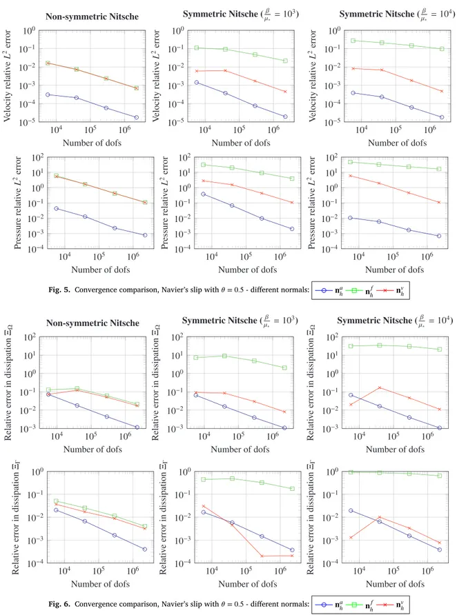
Fig.5.Convergencecomparison,Navier’sslipwith𝜃 =0.5-differentnormals:

Fig.6.Convergencecomparison,Navier’sslipwith𝜃 =0.5-differentnormals:

Ξ[J∕s]=ΞΩ+ΞΓ= 8𝜋𝜃𝑉2_𝑅𝐿𝜇 ∗ [ 4𝛽∗(1−𝜃)+𝜃𝑅 ] , (74) 𝐽𝑝[J∕s]=𝐺𝐿_∫ Γ_in𝐯⋅ 𝐧 d𝑆=−𝐺𝐿𝜋𝑅2_{𝑉, (75)} 𝑝drop[Pa]=𝑝𝑖𝑛−𝑝𝑜𝑢𝑡=𝐺𝐿= 8𝜃𝑉𝐿𝜇∗ 𝑅[4𝛽∗(1−𝜃)+𝜃𝑅 ]. (76)

Moreover,wedefinethe𝐿1_{-normofthevorticityby}

‖rot𝐯‖1[m3∕s]=_∫ Ω || || | ( 𝜕𝜔 𝜕𝑦,−𝜕𝜔𝜕𝑥,0 )_|| || |d𝑥= 8𝑉𝜃|Ω| 3[4𝛽∗(1−𝜃)+𝜃𝑅 ] = 8𝜋𝑅 2_𝐿𝑉𝜃 3[4𝛽∗(1−𝜃)+𝜃𝑅 ] (77)

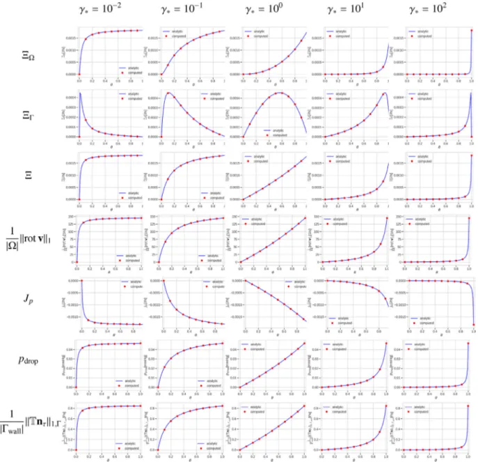
Fig.7. ComparisonoftheanalyticalandcomputeddissipationsΞΩ,ΞΓ,Ξ,pressuredrop𝑝drop,pressureflux𝐽𝑝and𝐿1normofvorticitydividedbyvolumeand𝐿1

normofwallshearstressdividedbywallareafortubulargeometrycomparedtotheanalyticalsolutionwithbenchmarkparametersdefinedinSection5.3.

andthe𝐿1_{-normofthewallshearstressby}

‖(𝕋𝐧)_𝜏‖1,Γwall[Pa.m 2_]= ∫Γwall |(𝕋𝐧)_𝜏| d𝑆=_[ 4𝜇∗𝑉𝜃|Γwall| 4𝛽∗(1−𝜃)+𝜃𝑅 ] = [ 8𝜋𝜇∗𝑉𝜃𝑅𝐿 4𝛽∗(1−𝜃)+𝜃𝑅 ]. (78) 5.3. Benchmarkparameters

Thegeometricalandflowparameterswerechosentobeascloseas possibletothoseforbloodflowintheaorticrootorasegmentof tho-racicaorta (motivatedbytheassessmentofclinical significanceof a

stenosedaorticvalve).Thegeometryconsideredisthatofa12mm ra-dius(24mmdiameter)cylinder.Thisisconsistentwithtypicalaortic di-mensions.Thegeometricaldatatogetherwiththedensity,thedynamic viscosityandtheinflowvelocityweretakenfromŠvihlová etal.(2017). ForgeometricaldataseealsoMadukauwa-Davidetal.(2018).

Therearetwoslipparametersprescribedonthewall,𝛾∗and𝜃,and

theyarerelatedtoeachother,see(40).Weusetheparameter𝛽∗=𝛾∗𝜇∗

asacharacteristiclengthofthegeometry,specifiedasradiusoftheinlet

𝑅.ThevaluesoftheconstantsandtheirunitsareshowninTable1.These valuesresultintheReynoldsnumber𝑅𝑒=𝑉𝑅𝜌∗

2𝜇∗

=1051.Twoprescribed functionsare𝐯in:=(0,0,𝜔(𝑥,𝑦))with𝜔(𝑥,𝑦)givenby(58)andtheoutlet

Fig.8. ComparisonoftheanalyticalandcomputeddissipationsΞΩ,ΞΓ,Ξ,pressuredrop𝑝drop,pressureflux𝐽𝑝,𝐿1normofvorticitydividedbyvolumeand𝐿1norm

ofwallshearstressdividedbywallareawithregardtotheparameter𝜃 fordifferent𝛾∗.Thesetwoparametersarerelatedtoeachotherthrough(7).

6. Results

Nextwecanlookatthenumericalresultsforthemodeldescribed in Section 2.1 as compared to the analytical solutions derived in

Section5.2.Thisgivesustheopportunitytoassesseveralaspectsofthe discretizationmethod.Firstofall,themeshconvergencecanbe com-paredforthesymmetricNitscheformulationwithdifferentpenalization parameters𝛽 andthenon-symmetricNitscheformulation.Then,witha selectedformulationwecomparethequantitiesofinterestforthefull scaleofboundaryconditionsfromfullslip(𝜃 =0.0)tonoslip(𝜃 =1.0).

6.1. Symmetricvs.non-symmetricNitscheformulation

Tables2–7summarizethebehaviorofthediscretesolutionwith re-specttothemeshrefinement.Thecomputationswerecarriedoutonthe sequenceof4regularlyrefinedmeshes.Fig.5collectstheconvergence behaviorforrelativeerrors ofvelocity𝐯andpressure𝑝in𝐿2 _norms

as ‖𝐯𝑎−𝐯ℎ‖𝐿2

‖𝐯𝑎‖𝐿2 and

‖𝐩𝑎−𝐩_ℎ‖_𝐿2

‖𝐩𝑎‖𝐿2 .Each graphcompares thebehaviorofthe

errorforthe3variantsofdiscretenormalvectors.Itisclearthatthe

analyticnormalgivesthemostaccuratesolution,howeverthisis avail-ableonlyinspecialcasesandcannotbeusedinageneralgeometry. Behaviorforthetwoothernormalsnowdependsonthevariantofthe Nitschemethodused.Thenon-symmetricNitschemethodgivesalmost thesameresultsforbothnormals– facetbasedandvertexbased.Inthe caseofsymmetricNitschemethodthevertexbasednormalgiveserrors comparablewiththenon-symmetricmethodbutthefacetbasednormal resultsinmuchlargererrorsandifthepenaltyparameterisnotchosen correctlyitseemstoconvergeatalowerrateofconvergence.

Fig.6portraysthesamecomparisonforthedissipation.Here the observationissimilar– namelythatthecombinationofthesymmetric Nitschemethodwiththefacetbasednormalleadstomuchlargererrors andslowerconvergencecompared toalltheothercombinations.We note thattheselectionof thevalueforthepenaltyparameter𝛽 was

givenbythefactthatforsmallervaluestheconvergenceisnotachieved, probablyduetolesserstability,andforhigherpenaltyparameterthe resultingaccuracydegrades.

Thefinalobservationisthattheresultsforthenon-symmetric vari-antoftheNitschemethodarenotsensitivetothechoiceofthenormal