HAL Id: hal-01899840
https://hal.archives-ouvertes.fr/hal-01899840
Preprint submitted on 19 Oct 2018
HAL is a multi-disciplinary open access
archive for the deposit and dissemination of sci-entific research documents, whether they are pub-lished or not. The documents may come from teaching and research institutions in France or abroad, or from public or private research centers.
L’archive ouverte pluridisciplinaire HAL, est destinée au dépôt et à la diffusion de documents scientifiques de niveau recherche, publiés ou non, émanant des établissements d’enseignement et de recherche français ou étrangers, des laboratoires publics ou privés.
Hossein Abbaspour, Francois Laudenbach
To cite this version:
Hossein Abbaspour, Francois Laudenbach. Morse complexes and multiplicative structures. 2018. �hal-01899840�
Hossein Abbaspour & François Laudenbach
Abstract. In this article we lay out the details of Fukaya’s A∞-structure of the Morse com-plexe of a manifold possibily with boundary. We show that this A∞-structure is homotopically independent of the made choices. We emphasize the transversality arguments that some fiber product constructions make valid.
Contents
1. Introduction 1
2. Multi-intersections towards A∞-structures 4
3. Compactification 12
4. Coherence 14
5. Transition 20
6. Orientations 23
7. A∞-structure 26
8. Morse concordance and homotopy of Ad-structures 29
Appendix A. Basics on homotopical algebras 33
References 35
1. Introduction
We are given an n-dimensional compact manifold M with boundary and a generic Morse function f : M → R, generic meaning that f has no critical point on the boundary and that the restriction f∂ of f to the boundary ∂M is a Morse function. For the purpose of the present
paper, it is useful to assume that M is orientable.
We recall that there are two types of critical points of f∂, those of Neumann type and those
of Dirichlet type; a critical point x of f∂ has type Neumann (resp. Dirichlet) if < df(x), n(x) >
is negative (resp. positive) where n(x) is a vector in TxM pointing outwards. We shall denote
by critkf the set of critical points of f (in the interior of M) of index k and by critNkf∂ (resp.
critD
kf∂) the set of critical points of f∂ of index k ∈ {0, . . . , n − 1} which are of Neumann type
(resp. Dirichlet type).
2000 Mathematics Subject Classification. 57R19. Key words and phrases. Morse theory, pseudo-gradient.
This setting was already considered in [15] where the main idea was to introduce so-called adapted pseudo-gradients, defined as follows. Below, we use notation slightly different from the cited paper.
A vector field XN is said to be N-adapted to f if the following conditions are fulfilled:
1) XN · f < 0 outside critf ∪ critNf ∂;
2) XN is pointing inwards at every point of ∂M except in some neighborhood of critNf ∂
where XN is tangent to the boundary; therefore, XN vanishes exactly at the points of
critf∪ critNf ∂;
3) near critf (resp. critNf
∂) the vector field XN (resp. XN|∂M) is the descending gradient
of f (resp. f∂) with respect to the Euclidean metric of some (unspecifized) Morse chart.1
Since the flow of XN is positively complete, each x ∈ critf ∪ critNf
∂ has an unstable manifold
Wu(x)whose dimension is equal to the index of x and a local stable manifold Ws
loc(x). Actually,
there is also a global stable manifold Ws(x)by taking the union of the inverse images of Ws loc(x)
by the positive semi-flow of XN.
The vector field is said to be Morse-Smale when all these invariant manifolds intersect mutu-ally transversely. Under this assumption, after choosing arbitrarily orientations of the unstable manifolds, one defines a graded complex
C∗(f, XN) = C∗N = CnN ∂N −→ · · · CN k ∂N −→ · · · CN 0 . Here, CN
k is the Z-module freely generated by critkf∪critNkf∂ and the differential ∂N is defined
by counting with signs the connecting orbits from x to y when the index of x equals ind(y) + 1 (notice that the local stable manifolds are co-oriented).
Similarly, a vector field XD is said to be D-adapted to f when it is N-adapted to −f. Notice
that XD · f > 0 apart from critf ∪ critDf
∂. Choose such an XD which is Morse-Smale and
choose an orientation of its unstable manifolds; they exist globally since the flow of XD is still
positively complete. One defines a second complex
C∗(f, XD) = C∗D =CnD−→ · · · C∂D kD−→ · · · C∂D 0D. Here, CD
k is the Z-module freely generated by critkf∪ critDk−1f∂. Notice the shift of the grading
which is justified by the equality:
CkD(f ) = Cn−kN (−f). The differential ∂D is defined on a generator x ∈ CD
k by counting with signs the connecting
orbits of XD from y ∈ CD
k−1 to x. The main result in [15] is the following.
Theorem 1.1.
1) The homology of the complex C∗(f, XN) is isomorphic to H∗(M ;Z).
2) The homology of the complex C∗(f, XD) is isomorphic to H∗(M, ∂M ;Z).
The labelling, Neumann or Dirichlet, comes from similar results which have been obtained previously in Witten’s theory of de Rham cohomology for manifolds with boundary (see [4, 10, 13]).
1In order to control the compactification of forthcoming moduli spaces, it is easier to reinforce the
In the present article, we present an important complement to Theorem 1.1 which deals with the multiplicative structures which exist on the considered complexes. Here we follow ideas which have been developed by K. Fukaya for closed manifolds (see [8] and also [3],[23]). Indeed, in [8] Fukaya has proposed the construction of an A∞-category whose objects are the smooth
functions on a given closed manifold M and the set of the morphisms Mor(f, g) is Z-module generated by the critical points of g − f. He describes the A∞-operations
mn: Mor(f1, f2)⊗ Mor(f1, f2)· · · ⊗ Mor(fn−1, fn)→ Mor(f1, fn)
by counting points with sign (orientation) on the zero-dimensional moduli space of flow lines intersection according to the scheme provided by a generic (trivalent) rooted tree.
These operations are only partially defined, meaning that the operation mn is only defined
for generic function fi’s. In particular, by taking fi = if, where f ∈ C∞(M )is a generic Morse
function, he suggested the existence of an A∞-structure on the Morse complex of f. Note that
in this example Mor(if, (i + 1)f)) is precisely the Morse complex of f. In this article, not only we give an accurate construction of the hitherto described A∞-structure on the Morse complex
of a Morse function f, but also we prove that this A∞-structure is well-defined up to
quasi-isomorphism of A∞-algebras. It turns out that the construction of A∞-quasi-isomorphisms
requires to extend Fukaya’s A∞-structure to manifolds with boundary.
Theorem 1.2. Here, M is supposed to be orientable and oriented. Then, each of the complexes CN
∗ and C∗D can be endowed with a structure of A∞-algebra A = {m1, m2, . . .} such that m1 is the
differential of the considered complex; here mddenotes the d-fold product. This structure is
well-defined up to “homotopy” from the data of a coherent family of Morse-Smale approximations of XN (resp. XD).
The approximations in question will be submitted to some transversality conditions for which the possible choices are not at all unique. The coherence (Definition 4.1) will be a form of naturality of these choices with respect to a certain group of diffeomorphisms of M.
The basic definitions about A∞-structures are recalled in Appendix A. As we shall see in
Section 8, the concept of homotopy of A∞-structures is the algebraic translation of the idea of
cobordism for the geometric objects we are going to introduce further.
The main example that we have in mind is 3-dimensional. Consider a link L in the 3-sphere S3, equipped with the standard height function h : S3 → R. The manifold with boundary we
are interested in is M := S3U(L), where U(L) is the interior of a small tubular neighborhood
of L, built by means of an exponential map. In general position of L, the height function induces a Morse function on L, and hence a generic Morse function f on M. Each maximum of h|L gives rise to a pair of critical points of f∂, one of Neumann type and index 2, and one of
Dirichlet type and index 1 (hence of degree 2 in CD
∗ ). Each minimum of h|L gives rise to a pair
of critical points of f∂, one of Neumann type and index 1, and one of Dirichlet type and index
0 (hence of degree 1 in CD
∗ ). It is reasonable to expect that the Morse complexes of this pair
(M, f ) informs a lot on the topology of L. We have not yet explored this topic systematically. As an exercise only, by using the Massey product which is derived from the third product of the A∞-structure on the Dirichlet type complex, one could prove à la Morse that the Borromean link is not trivial.
Sections 2 to 6 are devoted to topological preparation to multiplicative structures by means of a large use of Thom’s transversality Theorem with constraints [22]. Here are some more details:
-Section 2 makes a list of transversality conditions which will be used for defining products of an A∞-structure. These conditions are generic.
-Section 3 deals with the compactification of the geometric objects introduced in Section 2. The simple structure of the respective compactifications guarantees the preceding transversality conditions to be open.
-Sections 5 and 4 treat refinements on transversality conditions allowing the products to satisfy the A∞-relations. This is the hardest part.
-Section 6 with the orientation of the moduli spaces. - In Section 7 we introduce the A∞
-structure and prove A∞-relations.
- Section 8 explains why different choices in the previous constructions lead to concordant multi-intersections. That is the topological ingredient for homotopy of A∞-structures.
The proof of Theorem 1.2 will be achieved in Sections 7 and 8. We should say that many authors have addressed the A∞-structures of the Morse complex in various articles (see [9, 1, 2]
for instance). As far as we know, their construction amounts to a pre-∞ category/Algebra and do not really propose a homotopy A∞-invariance of the construction. The other authors
have treated the transversality issues using more analytical methods, such as moduli space of gradient trees, which are rather heavy when it comes to verifying the details. That is the reason why we have made efforts to provide a more topological and standard method. In particular we have tackled the difficulties relevant to the transversality issues by introducing a construction based on iterated fiber products.
Acknowledgements. The second author is deeply grateful to Christian Blanchet who led him to this topic many years ago.
2. Multi-intersections towards A∞-structures
In this article, we only consider the case of the boundary relative theory dealing with the Dirichlet type critical points and adapted gradient XD. Similar results hold true for the
Neu-mann type complex. In contrast with [15] where critical points in critf ∪ critDf
∂ are only
equipped with local stable manifolds, we shall here make use of global stable manifolds of criti-cal points. Since the flow of XD, denoted by ¯XD
t at time t, is positively complete, the following
definition makes sense:
Definition 2.1. For x ∈ critf ∪ critD(f
∂), the global stable manifold of x with respect to XD
is defined as the union
Ws(x, XD) = t>0 ¯XD t −1 Wlocs (x, XD).
Under mild assumptions, Ws(x, XD) is a (non-proper) submanifold with boundary and its
closure is a stratified set. Here is such an assumption (Morse-Model-Transversality) which is made in the rest of the paper.
(MMT) For every x ∈ critf ∪ critDf
∂ and y ∈ critDf∂, the neighborhood Uy of y in ∂M where
XD is tangent to the boundary of M is mapped by the flow transversely to Ws
As XD is Morse-Smale, the transversality condition is satisfied along a small neighborhood
U of the local unstable manifold Wu
loc(y, XD). Then, after some small perturbation of XD
on Uy U destroying partially the tangency of XD to ∂M, Condition (MMT) is fulfilled for
the pair (y, x). Thus, Condition (MMT) is generic among the D-adapted vector fields. The following proposition can be proved easily.
Proposition 2.2.
1)Under Condition (MMT), the global stable manifold Ws(x, XD)is a submanifold with
bound-ary (not closed in general).
2) If z belongs to the closure of Ws(x, XD), then there exists a broken XD-orbit from z to x.
The number of breaks defines a stratification of this closure clWs(x, XD).
For the rest of this section, we consider a generic Morse function f : M → R and a pseudo-gradient XD which is D-adapted to f. The transversality conditions Morse-Smale and (MMT)
are assumed.
We now turn to A∞-structures for which we refer to B. Keller [12]. In ([8, 9]), K. Fukaya
had proposed the construction of such structures on the Morse complexes of a closed manifold. We adapt his ideas to the case of M, a manifold with non-empty boundary. The main point is to parametrize multi-intersections by trees. First, we are going to define the trees under consideration, that we call Fukaya trees.
Definition 2.3. Let d be a positive integer. A Fukaya tree of order d (or a d-tree) is a finite rooted tree with d leaves which is properly C1-embedded in the unit closed disc D. The end
points (the root and the leaves) lie on the boundary ∂D. The rest of the tree lies in the interior of D. By a vertex we mean an interior vertex; it is required to have a valency greater than 2. An interior edge has its two end points in int D. Each edge is oriented from the root to the leaves.
Let Td be the set of Fukaya d-trees. There is a natural C1 topology on this set. The
ε-neighborhood of T0 ∈ Td is the set of Fukaya trees T equipped with a simplicial map ρ : T → T0
such that each edge α of T is embedded C1-close to the embedding of ρ(α) (which is an edge or
a vertex). This topology is a topology of infinite-dimensional manifold (Stasheff). But, up to isotopy (not ambient isotopy, due to moduli of angles), there are finitely many representatives only. From this fact it is possible to derive a stratification of Td where the number of interior
vertices is fixed on each stratum. In a generic tree all vertices have valency 3 (codimension 0 stratum). A codimension-one stratum in Td is made of trees all of which vertices have valency
3 except one which has valency 4.
Definition 2.4. Given the pair (f, XD), a decoration D of a Fukaya tree consists of the
fol-lowing: with each edge e of T , interior or not, one associates some approximation Xe of XD
which will be generic among the pseudo-gradients D-adapted to approximations2 of f.
Some mutual transversality conditions will be specified in Section 5. For the time being, we just list the needed conditions. Since the successive manifolds we are going to construct have natural compactification, all required transversality conditions will be not only dense but also open.
In the construction right below, we will use the positive semi-flow ¯Xe : [0, +∞) × M → M
of Xe. But for compactification purposes, it is more convenient to consider the graph of the
semi-flow in the following sense.
Definition 2.5. The graph G( ¯Xe)of the positive semi-flow ¯Xe is the part of M ×M made of the
pairs (x, y) such that y belongs to the positive half-orbit of x, that is: there exists t ∈ [0, +∞) such that y = ¯Xe(t, x). Since Xe is a pseudo-gradient, this time t is unique if x is not a zero of
Xe.
The graph contains the diagonal of M × M. For a pseudo-gradient semi-flow, the graph is a non-proper (n + 1)-dimensional submanifold, except at the points (a, a) where a is a zero of Xe. Its compactification will be discussed in Section 3 (in particular, Proposition 3.2).
The first projection M × M → M induces σe : G( ¯Xe)→ M which is called the source map.
The second projection induces τe : G( ¯Xe)→ M which is called the target map. These two maps
have a maximal rank, except at the points (a, a) as above.
Example 2.6. Let Q : Rn → R be the quadratic form of Morse index k and rank n:
Q(x1, . . . , xn) =−x21− . . . − x2k+ x2k+1+ . . . + x2n.
After taking local closure, the graph of the semi-flow of ∇Q looks like, for k = 1, . . . , n, the R-cone over an n-dimensional band (that is, ∼=Rn−1× [0, 1]) bounded by two affine subspaces: one is (−1, Rk−1, 0, . . . , 0)× (0, . . . , 0, Rn−k)⊂ Rn× Rnand the other is the part of the diagonal
over {xk =−1}. For k = 0, it is similar (change Q to −Q). See Figure 1.
{x = 1}
n = 1, k = 1 n = 1, k = 0
Figure 1.
2.7. Multi-intersection modelled on T . A construction. We are given a generic Fukaya d-tree T , with a decoration D, and d entries (x1, . . . , xd)where each xi belongs to critf ∪critDf∂.
The entries decorate the leaves of T clockwise. With these data we want to associate a manifold
(2.1) I(T,D, x1, . . . xd)⊂ M×n(T ) where n(T ) = d − 1.
Note that n(T )−1 = d−2 is equal to the number of interior edges. The reason of that dimension will appear along the construction. This manifold, called the multi-intersection modelled on T
or the T -intersection of the given entries, should be considered as a generalized intersection of the stable manifolds prescribed by (x1, . . . xd) and the pseudo-gradients listed in D.
The intersection process works as follows. With each edge e of T we are going to associate a generalized stable manifold Ws(e)and with each interior vertex v we are going to associate a
multi-intersection I(v) by applying the next rules inductively.
Rule 1. The edge ei ending at the i-th leaf is given the entry xi and is decorated by the vector
field Xei. This data yields the stable manifold W
s(x′
i, Xei) where x′i is the unique zero of Xei close to xi provided by the Implicit Function Theorem. One sets
Ws(ei) := Ws(x′i, Xei). Rule 2.
Let v be a vertex which is the starting point of ei and ei+1; there always exists such an i
except when T has no vertex. It is assumed that, whatever the entries are, the intersection I(v) := Ws(ei)∩ Ws(ei+1)
is transverse. Since there are finitely many entries, this transversality condition is easily ful-filled, at least when xi ∕= xi+1. The case xi = xi+1 raises some difficulty: the decoration of ei+1
has to differ from that of ei (compare Section 5).
The edge e ending at v is decorated by Xe. We consider the graph Ge := G( ¯Xe)of its positive
semi-flow ¯Xe, in the sense of definition 2.5. Let τe: Ge → M be its target map.
Rule 3. We define the generalized stable manifold Ws(e)as the fiber product
Ws(e) := limGe τe
−→ M←− I(v)j ,
where j denotes the inclusion I(v) → M. We have Ws(e) ⊂ M × M. It is endowed with a
source map which is induced by the source map σe of Ge. Note that σe is the restriction to
Ws(e)of the first projection p
1 : M × M → M.
Generically on Xe, that vector field has no zero on I(v). Then, since τe has maximal rank,
Ws(e) is a (non-proper) submanifold, whatever the entries are; it is said to be transversely
defined.
Nevertheless, the source map σe : Ws(e) → M is not immersive in general (due to the
tangencies of Xe with I(v)). Generically on Xe, this is an immersion almost everywhere.
Hence, the question is: how to make further intersections?
Let v′ be the origin of the above-mentioned edge e. First, consider the particular case where
v′ is also the origin of ei−1. It is assumed that I(v) is transverse to Ws(ei−1) (a new
transver-sality condition).
Rule 4. The multi-intersection I(v′)is defined as the fiber product
I(v′) := limWs(ei−1) j
−→ M σe
←− Ws(e), where j stands for the inclusion Ws(e
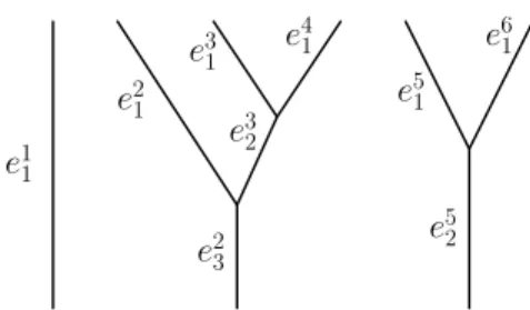
e1 e2 e0 v1 v2 v0 T (e2) Figure 2.
It becomes natural to ask the following question: under which transversality condition this fiber product is a manifold? Observe that I(v) is not moving when Xe is perturbed; as a
consequence, the requirement Ws(e
i−1)⋔ I(v) is a necessary condition.
Assume that condition. Then, generically on Xe, the restriction σe|Ws(e) of the source
map is transverse to Ws(e
i−1), whatever the entries are. Indeed, this follows from Thom’s
transversality theorem with constraints [22].
In that case, the fiber product is said to be transversely defined. It is a smooth submanifold I(v′) in Ge ⊂ M × M endowed with the projection pv′ : I(v′) → M induced by σe. That projection is again the restriction of the first projection p1 : M × M → M. This I(v′) is the
desired intersection, in our particular case. We introduce some notations and then we shall ready for an inductive construction.
If e is an interior edge in T , we denote T (e) the subtree of T rooted at the origin of e and containing e. Then, the integer n(e) is defined so that n(e) − 1 is equal to the total number of interior edges of T lying in T (e). If e is not interior and ends in a leaf, one takes n(e) = 1.
If v0 is an interior vertex of T , the integer n(v0) is defined so that n(v0)− 1 is equal to the
total number of interior edges above v0 with respect to the orientation of the tree from the root
to the leaves. Let e1, e2 be the two edges starting from v0 clockwise. The part of T rooted at
v0 will be denoted as a bouquet T (e1)∨ T (e2). One checks the formula
(2.2) n(v0) = n(e1) + n(e2)− 1
If e0 is the edge ending in v0 and e0 does not start from the root of T , we have
(2.3) n(e0) = n(v0) + 1
In what follows, we choose to denote the first projection of M×k → M by p
1 whatever k is.
We now start with the inductive construction. Denote by v1 and v2 the respective end points
of e1 and e2 (see Figure 2). The inductive assumptions are those stated from (2.4) to (2.6):
(2.4) The multi-intersection I(vj)is transversely defined as a submanifold of M×n(vj).
(2.5) The generalized stable manifold Ws(e
j)is transversely defined as a submanifold of
Each of these stable manifolds is endowed with a source map σj := σej to M which is again the restriction of the first projection p1 : M×n(ej) → M.
Assume also that the two following maps are transverse, that is: (2.6) p1|Ws(e1)⋔ p1|I(v2),
meaning that their product is transverse to the diagonal of M × M.
Be careful that the first projections p1 in the above formulas have not the same source in
general. Under these assumptions, Thom’s transversality theorem tells us that, generically on the decoration Xe2, the respective source maps σ1 and σ2 are mutually transverse. Thus, the next rule holds:
Rule 5. The multi-intersection I(v0), denoted by I (T (e1)∨ T (e2)), is transversely defined by
the fiber product
(2.7) I(v0) := lim Ws(e1) σ1 −→ M σ2 ←− Ws(e2) .
This is a submanifold of M×(n(e1)+n(e2)−1) = M×n(v0). It is endowed with a projection p
v0 : I(v0)→ M, which is the common value of σ1 and σ2 on this intersection. By convention, the
base of a fiber product can always be put as the first factor of the product. Thus, this common value is the restriction of p1 : M×(n(e1)+n(e2)−1) → M.
The edge e0 ending at v0 is decorated with a pseudo-gradient Xe0. Let Ge0 be the graph of its semi-flow and let τe0 : Ge0 → M be the target map. Generically on Xe0, its zeroes are not in the image pv0(I(v0)). Hence, τe0 is transverse to pv0|I(v0). Thus, the next rule holds:
Rule 6. The generalized stable manifold Ws(e
0) is transversely defined by (2.8) Ws(e0) := lim Ge0 τe0 −→ M←− I(vpv0 0) .
This fiber product is a submanifold of M×n(e0). The first projection of the latter product induces the projection σe0 : W
s(e
0)→ M.
For allowing us to pursue the construction inductively, it is necessary to assume some transversality conditions similar to the one expressed in (2.6). This condition is, a priori, generically satisfied by approximation of all previous decorations. More details will be given later on (Proposition 4.2); actually, all generic choices may be done inductively (Section 5).
Finally, let eroot= eroot(T )be the edge starting from the root of T and let v1root= vroot1 (T ) be
its interior vertex. Arguing inductively as above, we have a generalized intersection (2.9) I(T ) := I(v1root)⊂ M×n(v1root) = M×n(T ).
In this notation, the decoration and entries are missing. We define the T -intersection of the entries (x1, . . . , xd)associated with the chosen decoration D by
I(T ) = I(T,D, x1, . . . xd) := I(vroot1 )⊂ M×n(T ).
It is endowed with a projection proot : I(vroot1 )→ M in the same way as I(v0)was endowed with
Proposition 2.8. (Dimension formula) (2.10) δ(T ) := dim I(T ) =
1≤i≤d
(dim Ws(xi)− n) + d − 2 + n .
Proof. If we consider the Fukaya tree T0 where all interior edges are collapsed, formula (2.10)
where d − 2 is erased (as there is no interior edge) reduces to the usual dimension formula for an intersection of d submanifolds: it is additive up to the shift by the dimension. Each time an interior edge is created, the dimension increases by 1 since some flow is used and generates
a stable manifold. □
All the above-described manifolds are oriented. The orientations will be specified in Section 6. They will play an important rôle in the A∞-structures with integral coefficients.
2.9. Multi-intersection as a chain. In order to see the above multi-intersection I(T ) as a chain of degree δ(T ) in the Morse complex CD
∗ (f ), we have to define the coefficient
< I(T ), xroot >for every test data xroot∈ critf ∪ critDf∂ of degree δ(T ). We insist to decorate
the edge eroot with the vector field XD itself. Of course, this choice requires the following
condition: (2.11)
The projection proot is transverse to the unstable manifold Wu(xroot, XD)
for every xroot.
Here proot : I(T )→ M is induced by the first projection p1 : M×n(T )→ M.
Lemma 2.10. Given a Fukaya tree T , a generic decoration of T yields a multi-intersection I(T ) which fulfills (2.11).
Proof. In the recursive construction of a decoration of T , we are allowed to add some new transversality condition at each stage. Namely, for every vertex v (resp. edge e) of T and every data xroot we demand I(v) (resp. Ws(Xe)) to be transversely defined and, in addition, to be
transverse to Wu(x
root, XD). This new requirement can be easily satisfied. □
2.11. T -evaluation map. By choice of the degree of the test data, the codimension of the unstable manifold Wu(x
root, XD) is equal to δ(T ). Then, the following multi-intersection
< I(T ), xroot) >:= lim
I(v1 root) proot −→ M←− Wj u(x root, XD) , is 0-dimensional, where j stands for the inclusion Wu(x
root, XD) ↩→ M. As it will be explained
in Section 3, it is a compact set, and hence finite, with an orientation. Here, it is important to specify the orientation convention: for every critical point z
(2.12) orWs(z)∧ orWu(z)= or(M ) .
Therefore, it makes sense to define < I(T ), xroot > as the algebraic counting of elements in
this finite set. The map < I(T ), − > from the right degree test data to Z will be called the T-evaluation map; it depends on the choice of the decoration of T .
Definition 2.12. Given a generic Fukaya tree T , a decoration D is said to be admissible if, whatever the entries and the test data are, all the multi-intersections (resp. stable manifolds) associated with vertices (resp. edges) are transversely defined as submanifolds of M×k for some
integer k, as well as the T -evaluation.
Admissibilty is easily seen to be a generic property. But it is useful that this property be open. This requires to compactify the various objects that we just introduced (multi-intersections and their stable manifolds). This will be done in the next section.
The end of the present section is devoted to extend the description of multi-intersection to the case of non-generic Fukaya trees. First, we specifiy what is a subtree.
Definition 2.13.
1) The ordered set of leaves in a Fukaya tree T is denoted by L(T ). Let T0 and T1 be two Fukaya
trees. A Fukaya embedding j : T0 → T1 is an injective, non surjective, simplicial map which
sends L(T0) to a consecutive subset of L(T1) increasingly. The image j(T0) is called a Fukaya
subtree of T1.
2) An edge e in a Fukaya tree T is said to be of generation k if the maximal number of edges in a monotone path of T linking the origin of e to a leaf is equal to k.
3) A vertex which is the origin of a generation-k edge and not the origin of an edge of higher generation is said to be of generation k.
Note that the generation-k edges are ordered from the left. Indeed, there is a first leaf of T which is the terminating point of a monotone path P ⊂ T with k edges. The first edge of P will be the first generation-k edge. Then, erase the subtree which is rooted at the origin of P and contains P , and start again.
If v0 is a generation-k vertex in T , it is the origin of edges e1, . . . , em, where m > 1 (at least
one ej is of generation k). Let v1, . . . , vm denote the respective end points of e1, . . . , em and
let T1, . . . , Tm be the subtrees rooted at v0 containing v1, . . . , vm respectively. As before, the
integer n(vj) is defined such that n(vj)− 1 is equal to the number of interior edges above vj.
The integer n(ej) := n(vj) + 1 is equal to the number of interior edges in T lying in Tj.
Definition 2.14. Let fj : Nj → M, j ∈ J, be a finite set of smooth maps from manifolds to
M. They are said to be transverse if, for every subset K ⊂ J, the product map j∈K fj : j∈K Nj → M|K|
is transverse to the small diagonal of the target.
In that case, the fiber product limj∈Jfj is said to be transversely defined. This is a smooth
submanifold of the product j∈JNj.
Note that in the usual definition one takes K = J.
Let us again consider a Fukaya tree T , not necessarily generic, with a decoration DT, that
is, the data of an approximation Xe of XD for each edge e in T . We are going to repeat the
inductive definition of multi-intersection for each vertex of T . For that, we look at the vertex v0 in the setting previously described.
Assume that the multi-intersections I(vj), j = 1, . . . , m, are transversely defined and are
submanifolds of M×n(vj). Generically on X
p1 is again the first projection p1 : M×n(vj) → M. Thus, the generalized stable manifold
Ws(e
j,DT)is transversely defined as the fiber product
(2.13) Ws(ej,DT) := lim Gej τej −→ M p1 ←− I(vj)
Therefore, this stable manifold is a submanifold of M×n(ej)and the restriction of the source map σej to this fiber product is nothing but the restriction of the first projection p1 : M×n(ej
)→ M.
Proposition 2.15. In the above setting, the extra following assumptions are made: (2.14) The family of maps p1 : I(vj)→ M
j∈{1,...,m} is transverse.
Then, without changing the decoration DT above the vertices vj, generically on the decorating
vector fields Xej, j = 1, . . . , m, the multi-intersection I(v0,DT) is transversely defined as the fiber product (2.15) I(v0,DT) := lim j Ws(ej,DT) p1 −→ M.
Moreover, I(v0,DT) is a submanifold of M×n(v0), where n(v0)− 1 is equal to the number of
interior edges in T1∨ . . . ∨ Tm, and its projection to M is the restriction of the first projection.
Proof. First, thanks to assumption (2.14), for each j = 1, . . . , m, generically on the gradient field Xej, the family
p1|I(v1), . . . , p1|I(vj−1), p1|Ws(ej, Xej)
is transverse. Once, this is done, it is available to put successively p1|Ws(ej, Xej) transverse to the preceding family p1|Ws(e1, Xe1), . . . , p1|W
s(e
j−1, Xej−1)
by generic approximation. In all cases, Thom’s transversality theorem with constraints applies. The rest of the statement is clear by counting the dimensions and applying the definition of the integers n(vj)and n(ej). □
Remark 2.16. Due to the compactness which will be proved in Section 3, each genericity condition in question in the previous statement is fulfilled in an open dense subset of the space of gradient vector fields.
3. Compactification In general, the stable manifolds Ws(x
i, XD) are not compact and the graphs Ge are never
compact. In this section, we analyse their individual compactification and how they contribute to the compactification of the multi-intersection I(T ). All these closures will be stratified. The codimension-one strata are of particular interest. This is explained in the subsequent proposi-tions.
Proposition 3.1. Let x be a critical point in critkf ∪ critDk−1f∂ and XD be a Morse-Smale
pseudo-gradient D-adapted to f. Then, the closure in M of the stable manifold Ws(x, XD)
is made of all points which are linked to x by an orbit or a broken orbit of XD. It is a
stratified set whose strata of positive codimension are stable manifolds of some critical points y∈ critℓf ∪ critDℓ−1f∂ with ℓ < k. The codimenion-one strata are obtained for ℓ = k − 1.
This is well known for closed manifolds [14]. The same proof gives the case of manifold with non-empty boundary. The proof of the following proposition is very similar by considering the flow in the Morse model near a critical point. In what follows, we omit to note the pseudo-gradient.
Proposition 3.2. Let G ⊂ M × M be the graph of the positive semi-flow ¯XD of the
pseudo-gradient XD. Then:
1) The closure cl(G) of G in M × M is made of all pairs of points (x, y) where y belongs to the positive orbit of x or any broken positive orbit starting from x.
2) This cl(G) is a stratified set whose strata of positive codimension are made of pairs of points (x, y) where x is connected to y by a broken orbit passing through a non-empty sequence of critical points in critf ∪ critDf
∂.
3) The codimension-one strata are made of pairs of distinct points (x, y) where x belongs to the stable manifold Ws(z) for some z ∈ critf ∪ critDf
∂ and y belongs to the unstable manifold
Wu(z).
From Example 2.6 (or Proposition 6.6), we know that the strata considered in 3) above are (non-closed) boundary component of G. Observe that the index of z has no effect on the codimension of the stratum.
Notice also that G is already a manifold with boundary and corners due to the fact that M × M is such a manifold (if ∂M ∕= ∅). Moreover, the diagonal of M × M lies in G as a boundary (except over the zeroes of XD). The list of strata described in the items 2) and 3)
does not include them. Under the transversality assumption (MMT) introduced in Definition 2.1, the stratification of stable manifolds and graphs behave nicely with respect to ∂M and all together form a stratification with conical singularities in the sense of [14].
These partial results are made more precise in the following proposition.
Proposition 3.3. Let T be a Fukaya tree with d leaves and let D be an admissible decoration (in the sense of Definiton 2.12). Then:
1) The closure of IT(D, x1, . . . xd)in M×n(T ) has a natural stratification whose singularities are
conical for every system of entries.
2) A codimension-one stratum H other than those coming from ∂M or the diagonal of M × M has the following form:
There exist j ∈ {0, . . . , d − 1} and a sub-tree T0 in T , with k leaves, a root v0 and an initial
edge e ending at the vertex v1, and there is a zero z of the pseudo-gradient Xe ∈ D decorating
e such that:
- (i) the dimension of IT0(D, xj+1, . . . , xj+k) is equal to the Morse index of z;
- (ii) the stratum H and its transverse conical structure are generated in I(T ) by iterated fiber products from the pair
Ws(z)× cWu(z)× MI(T0) , Ws(z)× {z} , where c(−) stands for the cone of (−).
Remark 3.4. Note that by (i) the fiber product Wu(z)×
MI(T0)is a finite set S. When taking
the orientations into account, S is a signed finite set and the sum of these signs is an algebraic multiplicity, say µ. Therefore, H can be seen with a boundary component of the closure of I(T )with mutiplicity µ.
Proof. We limit ourselves to the case of generic trees. In order to determine the closure of I(T ) one follows the recursive construction 2.7 . As a result, the closure of I(T ) is itself the iterated fiber product of the closures of the factors. Thus, we have to check that, at each step the projection maps, restricted to strata in factors, are mutually transverse. That follows from the fact that the transversality conditions for multi-intersections are required to be fulfilled for every system of entries.
Concretely, when looking at the step mentioned on Figure 2 and assuming that the closures of Ws(e
1), Ws(e2) are stratified with conical singularities, the following is required: for each
pair of strata (A1, A2) where Ai is a stratum of the closure of Ws(ei), i = 1, 2, the restricted
source maps σ1|A1 and σ2|A2 are transverse. By fiber product diagram chasing, we get that
B := A1×
MA2 is a stratum of codimension k1 + k2 in the closure of IT(v0) where ki is the
codimension of Ai in cl
Ws(e
i)
. The singularities are conical by products and intersection with the diagonal of M × M.
For looking at what happens through the stable manifold Ws(e
0), we limit ourselves to the
case of a stratum of codimension one neither generated by ∂M nor by the diagonal ∆M. If B
from above is of codimension one in clIT(v0)
one can pursue the process of fiber products and B generates a codimension-one stratum in IT.
For having a new phenomenon, we need to start with I(v0)itself and consider, in the closure of
Ws(v
0), a stratum of broken orbits generated by a zero z of the vector field Xe. By admissibility
of the decoration, the embedding of Wu(z)into M is transverse to the projection p
v0 : IT(v0)→ M. Then the part of IT(v0) over Wu(z) is a submanifold S whose codimension is equal to the
Morse index of z.
If the dimension condition (i) is fulfilled, S is a finite set. Taking the pull-back to the graph Ge of the semi-flow ¯Xe and then the closure produces a bundle over Ws(z) which contains
Ws(z)× {z} and whose fiber is c(S) (adapt [14, Lemma 4] to the fiber product setting).
Therefore, Ws(z)× {z} appears as a boundary component of the closure of Ws(e) in M × M
with multiplicity and (ii) is fulfilled.
If S were not zero-dimensional, the top of the above-mentioned cone would be of codimension larger than one in c(S), and hence, H would not be of codimension one in clI(T ). □
Corollary 3.5. The admissible decorations of a given Fukaya tree form a dense open set among all decorations.
Proof. Let D be an admissible decoration of the generic Fukaya tree T . At each step of the construction 2.7, one looks at the strata of highest codimension first. They are closed, hence compact. Transversality along a compact set is an open property. As the singularities of the stratification are conical, transversality along a stratum S implies the following local transver-sality in a neighborhood N(S) of S in the ambiant manifold (which is some product M×k). For
each stratum S′ having S in the closure, transversality along S′ ∩ N(S) holds true. But the
complement in S′ of an open neighborhood of the frontier cl(S′) S′ is compact. We use again
4. Coherence
In this section, all Fukaya trees will be generic or not. The A∞-structure that we want to
reach requires to consider all Fukaya trees and to decorate them in a coherent way. We give the precise definition right below.
Definition 4.1. 1) Two admissible decorations of T are said to be isotopic if they lie in the same arcwise connected component of admissible decorations.
2) Assume that T0 and T1 are given admissible decorations D0 and D1 respectively. The two
decorations are said to be coherent if, for any Fukaya embedding j : T0 → T1 (in the sense of
Definition 2.13), the induced decoration j∗D
1 is isotopic to D0.
3) A system of admissible decorations {D(T )}T for all generic Fukaya trees is said to be coherent
if for any pair (T0, T1) of Fukaya trees the corresponding decorations D(T0) and D(T1) are
coherent.
We consider the group G = Diff0(M )of smooth diffeomorphisms of M isotopic to IdM. We
have chosen from the beginning a Morse-Smale vector field XD thanks to which some Morse
complex was built which calculates the relative homology H∗(M, ∂M ;Z).
Notation 4.2. Denote by Σ the union of unstable manifolds Wu(x, XD) of positive
codimen-sion, x ∈ critf ∪ critDf
∂. And similarly, Σ∗ denote the union of stable manifolds Ws(x, XD)
of positive codimension. Both Σ and Σ∗ are stratified submanifolds of M with conical
singu-larities. Let GΣ denote the connected component of Id in the subgroup of G which consists of
diffeomorphisms preserving the stratified set Σ. Recall that T1 (resp. T2) denotes the unique
tree with one leaf (resp. two leaves).
Proposition 4.3. Let d be a fixed positive integer. Then, for every g in some open and dense subset of GΣ, the sequence S = (Dk1)dk=1 of decorations T1 defined by
(4.1) D11 = XD,D12 = g∗XD, . . . ,Dj1 = g◦(j−1)∗ XD, . . . ,D1d= g∗◦(d−1)XD
has the following properties: 1) The family Ws(D1
1), . . . , Ws(D1d)
is transverse whatever the entries are. Moreover, this family is transverse to Σ, that is, to every unstable manifold contained in Σ.
2) For every integer j, 1 ≤ j < d, the decoration of T2 with Dj(T2) := (D1j,D j+1
1 , g∗◦(j−1)XD),
for the left branch, the right branch and the trunk respectively, is admissible. The decoration Dj(T
2) is isotopic to D1(T2) in the space of admissible decorations of T2. In particular, the
family {Dj(T
2)}j≤d−1 is coherent.
First, we need some lemma involving a more simple setup.
Lemma 4.4. Let N′ (possibly empty) and N be two transverse compact submanifolds of M of
positive codimension. Let GN′ denote the subgroup of G made of diffeomorphisms leaving N′ invariant. Then, the following property is generic for g ∈ GN′:
âĂŤ for every positive integer d, the family of embeddings {g◦j : N → M}d−1
j=0 is transverse
(in the sense of Definition 2.14); âĂŤ this family is transverse to N′.
Proof. We recall the following classical fact wich is a part of the so-called Kupka-Smale The-orem (see J. Palis & W. de Melo’s book [18, Chap. 3]): For a generic g ∈ GN′, all periodic points of g whose periods are less than d are non-degenerate. In particular, they are isolated. Therefore, generically, they do not lie in N.
First, we assume N′ is empty; in that case G
N′ = G. As usual for proving a transversality theorem with constraints, it is sufficient to prove that the statement holds when replacing g with a smooth finite dimensional family in G passing though g. Indeed, Sard’s theorem says that, if the statement holds for a family, it holds for almost every element in that family. We do it when d = 3; the general case is similar with more complicated notations. We have to prove that generically the following intersections are transverse:
(i) The triple intersection Θg := N∩ g(N) ∩ g◦2(N )is transverse;
(ii) The intersections N ∩ g(N) and N ∩ g◦2(N )are transverse.
We limit ourselves to prove the first item. The desired transversality condition is the following: The map
(4.2) g : N˜ (x, y, z)× N × N −→→ (x, g(y), gM × M × M◦2(z))
is transverse to the so-called small diagonal δ ⊂ M × M × M. This property is open by compactness of N. We have only to prove that it is satisfied on a dense set of G. We start with an element g ∈ G having its periodic points apart from N. We search for a family Γ ⊂ G passing through g and having the triple transversality condition (4.2). We first need to find a set of parameters.
If x0 ∈ Θg, there exists (y0, z0) ∈ N × N such that x0 = g(y0) and x0 = g◦2(z0). By
assumption on g, these three points are mutually distinct. Then, there is a finite coverings of Θg by Euclidean closed balls {Bj}qj=1 with the following property: denote by Bj′ and Bj′′ the
respective preimages of Bj by g and g◦2; if Bj is small enough, Bj, Bj′ and Bj′′ are mutually
disjoint. Each of these balls and their preimages are thought of as contained in an open chart. Our space of parameters will be (Rn, 0)q× (Rn, 0)q, where n = dim M and (Rn, 0) stands for a
small neighborhood of the origin in Rn.
For sj a small vector in the coordinates around Bj, the deformation gsj of g is defined by gsj(y) = g(y) + sj when y ∈ Bj′ and gsj(y) = g(y)when y lies outside some small neighborhood of B′
j given in advance.
Similarily, for tj a small vector in the coordinates around B′j, the deformation gtj is defined by gtj(z) = g(z) + tj when z ∈ Bj′′ and gtj(z) = g(z) when z lies outside some small given neighborhood of B′′
j. Notice that, for z ∈ Bj′′,
(gtj)◦2(z) = g(g(z) + tj).
If s = (s1, ..., sq) and t = (t1, ..., tq) are two q-tuples of small vectors in Rn, the announced
family Γ = gs,t is any family in G which coincides with gsj (resp. gtj) on the sj-axis (resp. on the tj-axis). As a map, Γ reads as the following:
(4.3) Γ : N × N × N × (R(x, y, z, s, t)n, 0)q× (Rn, 0)q −→−→ M × M × M x, gs,t(y), (gs,t)◦2(z)
We are going to show that this map is transverse to the small diagonal δ. More precisely, we are going to check that, for every triple (x, y, z) such that x = g(y) = g◦2(z), the restricted map
(s, t)∈ (Rn, 0)q× (Rn, 0)q −→gs,t(y), (gs,t)◦2(z)
is a submersion valued in M ×M. The triple (x, y, z) belongs to some triple of balls (Bj, Bj′, B′′j).
Thus, we restrict to s = sj and t = tj, the other translation coordinates being equal to 0. The
jacobian matrix J at (x, y, z, 0, 0) reads: J =
IdTxM 0 0 dg(g(z))
where dg(g(z)) : TyM → TxM is the tangent map to g at the point y = g(z). Finally, J is
an epimorphism. That finishes the proof that Γ is transverse to the small diagonal in the case when N′ is empty; if N′∩ N = ∅, the proof is the same. We are left with the case N′ ⋔ N ∕= ∅.
Let K denote the transverse intersection N′∩ N. We first have to put the triple intersection
K∩ g(K) ∩ g◦2(K) in transverse position in N′. This can be done according to the preceding
proof by replacing (N, M) with (K, N′). Just observe that the restriction G
N′ → Diff0(N′) is a fibration. Automatically, the transversality we get along N′ extends to transversality in some
neighborhood of N′.
Now, we are reduced to put in transverse position the triple intersections which do not ap-proach N′. Notice that, when x = g(y) = g◦2(z) /∈ N′, then y and z are not in N′ since g
preserves N′. For such triple points, the preceding proof works as if N′ were empty. This
finishes the proof of Lemma 4.4. □
We notice that the statement of Lemma 4.4 extends to the case where N and N′ are
subman-ifolds with conical singularities. We briefly indicate how the proof has to be changed. First, we consider the case when N′ =∅. The domain of the map Γ in formula (4.3) is a stratified set.
Thus we have to check that when A and B are two submanifolds with conical singularities of M, then A × B is a submanifold with conical singularities in M × M. Namely, if some stratum S ⊂ A (resp. S′ ⊂ B) has a link3 L (resp. L′), the link of the product S × S′ is the join L ∗ L′.
Now, if the domain of Γ is stratified with conical singularities, if σ is one of the strata and if Γ|σ is transverse to the small diagonal of the target, then the same holds near σ for each stratum τ having σ in its closure. Therefore, we are allowed to argue on each stratum of the domain of Γ inductively on the increasing dimension.
In the case where N ⋔ N′ ∕= ∅, we look at each smooth stratum σ of N′. Considering
K := N ⋔ σ as a submanifold with conical singularities in σ, we are able to realize the required transversality if it is already realized along every stratum in the frontier ¯σ σ. Again, arguing inductively, we are done with the stratified extension of Lemma 4.4.
Proof of Proposition 4.3.
1) The Morse-Smale property of the vector field XD implies that Σ∗ and Σ are two
trans-verse submanifolds with conical singularities. Then, we are allowed to apply Lemma 4.4 in its generalized form by taking N = Σ∗ and N′ = Σ. It tells us that for a generic g ∈ G
Σ and for 3 For x ∈ S, the intersection of A with a neighborhood of x in M reads S × cL where L is a submanifold
with conical singularities in the r-sphere, r = dim M − dim S − 1, and where cL stands for the cone on L in the (r + 1)-ball.
any entries, the intersection Ws(g◦(j−1)
∗ XD)∩ Ws(g◦j∗ XD) =: Ws(D1j)∩ Ws(D j+1
1 )is transverse.
Moreover, by 2) of Lemma 4.4, this intersection is transverse to Σ. This proves the first item. 2) Let us prove first the admissibility of D1(T2). Set I1
1 := Ws(D11) ⋔ Ws(D12). Consider
the intersection Wu(XD)⋔ I1
1. Its transversality follows from the first item. Thus, the inverse
image p−1
2 (I11) by the target map p2 is transverse to p−11 (Wu(XD)) in M × M at any point of
the diagonal.
The intersection G( ¯XD)∩ p−1
2 (I11) is transverse since there are no zeroes of XD in I11 (the
stable manifold associated with the trunk is transversely defined). We have to check that p−11 (Wu(XD)) intersects transversely G( ¯XD)∩ p−12 (I11). A point (x, y) in that intersection
satifies: x ∈ Wu(XD), y ∈ I1
1 and y = ¯XtD(x) for some t ≥ 0. As Wu(XD) is positively
invariant by the flow, we have y ∈ Wu(XD), that is, y ∈ Wu(XD)∩ I1 1.
The lifted flow ¯XD × Id
M to M × M preserves the three submanifolds the intersection of
which we are looking at. As said above, their mutual transversality holds in (y, y), and hence it holds in (x, y). This is the desired admissibility of D1(T2). The admissibility of Dj(T2) will
follow from the isotopy argument which is given right below.
For the second part of 2), observe that g◦(j−1) is a common factor in the three decorations
which appear in Dj(T2). Recall g is isotopic to Id
M by an isotopy (gt)t∈[0,1] which keeps Σ
invariant. Decompose g◦j = g◦(j−1)◦ g, apply the isotopy to the left factor, namely g◦(j−1) t , and
keep the right factor g unchanged. Along the isotopy, all the required transversality conditions are preserved since the triple of decorations are moved by an ambient isotopy. Therefore, this is an isotopy of admissible decorations, which is the statement of the second item. □
We are going to generalize Proposition 4.3 to any forest in the following sense.
Definition 4.5. 1) The height of a tree is the generation of its root (see Definition 2.13). In this subsection, the trees are drawn in the upper half-plane with roots in R× {0}. By definition, the root of a tree T belongs to one edge only; this edge is called the trunk of T (denoted by eroot(T ) in Subsection (2.7). The other edges of T are its branches.
2) A forest of height h is a finite union of pairwise disjoint trees of height ≤ h with at least one tree of height h.
Any height-h forest F yields a height-(h−1) forest c(F ) just by erasing a small neighborhood of all generation-h trunks and descending the newly created roots to R × {0}. This process can be iterated and yields successively c2(F ), c3(F ) and so forth.
4.6. Labeling of the edges and g-standard decoration. Denote by F(d) the set of forests with d leaves at most. For F ∈ F(d), the j-th leaf of F determines a unique maximal monotone path Pj(F )in F ending to that leaf. If e is an edge of F , it will be labeled ej
h(F )(or e j
h when no
possible confusion) if h is the generation of e and j labels the leftmost path Pj(F ) containing
e (see Figure 3). Observe (e.g. on this example) that for a given h > 1, any j ∈ [1, d] cannot appear as label of an edge of F .
e1 1 e2 1 e3 1 e 4 1 e5 1 e2 3 e3 2 e6 1 e5 2
Figure 3. A height-3 forest with 6 leaves
Recall the group GΣ of diffeomorphisms of M which are isotopic to IdM by an isotopy keeping
Σ invariant. For g ∈ GΣ, the g-standard decoration of F consists of decorating ejh(F ) with the
vector field g◦(j−1)
∗ XD. The multi-intersection associated with the vertex (of generation h − 1)
which lies at the end of ej
h(F ) will be denoted by I j h(F ).
Remark 4.7. If T is a subtree of F , there are two natural decorations on T : the first one is Dg(T ), the own g-standard decoration of T ; the second one is Dg(F )
|T which is induced on
T from the g-standard decoration of F . The question of coherence amounts to compare these two decorations on T . In this aim, what follows is helpful: if ej
1(F ) is the leftmost edge of
generation 1 sitting in T , then g◦(j−1)
∗ is a common factor to every edge decoration in Dg(F )|T.
The next lemma is the technical part for proving that, generically, the g-standard decoration is admissible and coherent.
Lemma 4.8. Given the number d of leaves, for every generation h, 1 ≤ h ≤ d, there exists an open dense subset Gh(d)⊂ GΣ such that the following two properties hold for every height-h
forest F ∈ F(d) and for every g ∈ Gh(d):
(4.4)
For every possible j, the map p1| Ws(ejh(F ), g∗◦(j−1)XD) is transverse to Σ and to
the family p1|Ws(eℓk(F ), g∗◦(ℓ−1)XD)
(k,ℓ) where k < h and (k, ℓ) runs among
all labels of branches of F, except those in the tree whose trunk is ej h(F ).
(4.5)
The family of maps p1| Ws(ejh(F ), g◦(j−1)∗ XD)
j, j running among
all possible labels, is a transverse family and, in addition, transverse to Σ.
In particular, if g ∈ Gh(d) the g-standard decoration makes all multi-intersections of F
trans-versely defined; that is, this decoration is admissible.
Proof.We prove this statement inductively on h. For h = 1, this is the first item of Proposition 4.3; let G1(d)denote the open dense set in question in that proposition. As a finite intersection
of open dense sets is still so, we may fix h and F ∈ F(d) in what follows.
Let us prove the statement for h = 2. About genericity of the condition (4.4), we limit ourselves to prove the genericity of transversality of p1|Ws(ej2(F ), g∗◦(j−1)XD) to one Ws(Dk1)
only, k ∕= j, j + 1. As openness of the condition is clear, we focuse on denseness. Then, we start with g1 ∈ G1(d) and we try to approximate it by g ∈ GΣ fulfilling the required transversality.
Denote by Φj
t the positive semi-flow of g∗◦(j−1)XD and take the g-standard decoration of every
considered edge. In that setting, (4.4) amounts to say that the equation whose unknowns are (x, t)∈ Ws(Dk
1)× R+:
(4.6) Φjt(x)∈ I2j(F )
is regular. This equation depends on g ∈ GΣ which plays the role of a parameter; it is hidden
in the domain of x and the intersection Ij
2(F ). By Proposition 4.3, for g close to g1 the
submanifolds Ws(Dk
1)and I21(F )are mutually transverse and their intersection is transverse to
Σ. That allows us to search maximal rank for the equation (4.6) by slightly deforming g in GΣ.
Note: firstly, Ws(Dk
1) can be thought of as being compact since all the entries of degree less
dim M are considered; and secondly, generically on g there are no zeroes of g◦(j−1)∗ XD lying in
I2j(F ). As a consequence, there are no solutions of (4.6) when t is large enough; (by reasoning on each stratum of Σ∗ âĂŤ see Notation 4.2 âĂŤ by decreasing codimension yields a uniform
bound for a possible t when g varies near g1).
When the parameter g is incorporated to the unknowns, the equation (4.6) extended to all g in a neighborhood of g1 is of maximal rank (already with respect to g) for (x, t) close to
some (x0, t0). By the above-noted compactness, we have only finitely many (x0, t0) to
con-sider. Therefore, we have a finite dimensional family G0 ⊂ GΣ passing through g1 such that
the equation (4.6) extended to G0 is of maximal rank. Then, by Sard’s Theorem, g1 can be
approximate by some g ∈ G0 where (4.6) has a maximal rank. Moreover, the transversality to
Σof the considered family (with the g-standard decoration) is for free as the approximation of g1 is made inside GΣ.
Regarding the condition (4.5), we limit ourselves to transversality of stable manifolds associ-ated with two trunks of generation 2 only, say ej
2(F ) and ek2(F ), k > j. For any i, let Φitdenote
the flow of g◦(i−1)
∗ XD. For a given g ∈ GΣ, (4.5) reads:
(4.7) Φjt1(x)∈ I2j(F ), Φkt2(x)∈ I2k(F ),
the unknows being (x, t1, t2) ∈ M × (R+)×2. The regularity of (4.7) could be discussed as we
did for (4.6). In particular, it is important to check there are no solution when one ti, i∈ {1, 2}
approaches +∞. It is not needed to say more about that condition.
About the induction from generation h−1 to generation h, it is not different from the passage from h = 1 to h = 2, except that having more complicated notation. More details seem not to
be needed. □
Proposition 4.9. Every forest F ∈ F(d) decorated with a g-standard decoration is admissible and coherent if g belongs to Gd(d) from Lemma 4.8.
Proof. The admissibility of such a decoration holds by Lemma 4.8. Concerning the question of coherence, suppose we are given F ∈ F(d) and a height-h sub-tree T ⊂ F . Let d′ < d the
number of leaves of T . Take any g ∈ Gd(d). This determines the g-standard decoration Dg(F )
of F , together with the induced decoration Dg(F )|
T on T , and also a decoration Dg(T ) of T
as Gd(d)⊂ Gh(d)for every h ≤ d. The question is to check that these two decorations of T are
Let ej
1(F ) be the leftmost generation-1edge of T ⊂ F . As noted in Remark 4.7, g∗◦(j−1) is a
common factor in the g-standard decoration of all edges of T : if eℓ
q(F ) is an edge of T , then the decoration of eℓ q(F ) reads g◦(ℓ−1)∗ XD = g∗◦(j−1) g∗◦(ℓ−j)XD .
Remember that g is isotopic to Id among the diffeomorphisms which preserve Σ. Let (gt)t∈[0,1]
such an isotopy, with g0 = g and g1 = IdM. Apply (gt)t to the factor g◦(j−1) while keeping
the other factors unchanged. This ambient isotopy of M carries decorations of all edges T accordingly. Every multi-intersection remains transversely defined and transverse to Σ. Thus, admissibility is kept throughout the isotopy.
Call D1(T ) the decoration of T at time t = 1 of the isotopy (g◦(j−1)t )t. By construction,
the generation-1 edges of T are decorated by XD, g
∗XD, ..., g◦(d
′−1)
∗ XD consecutively. Since the
monotone paths descending from the leaves to the root of T determined the decoration of T at time t = 0, this remains true at time t = 1 of the isotopy. As a consequence, D1(T ) is the
g-standard decoration of T . The coherence property is proved. □ 5. Transition
Proving A∞-relations in Section 7 requires analysing the transition phenomenon from I(T′)to
I(T′′), where T′and T′′are two generic Fukaya trees with d leaves on each side of a
codimension-one stratum in the space Td of Fukaya trees with d leaves (see Definition 2.3).
5.1. Setting of the transition. We consider two Fukaya trees T′ and T′′ which differ only in
the star of v (see Figure 4). The intermediate Fukaya tree T has codimension one since v has valency 4. Up to isotopy, T′ and T′′ are the only two possible deformations from T to a generic
Fukaya tree. The edge e′ (resp. e′′) is collapsed in T′ → T (resp. T′′ → T ). The counting of
interior edges gives n(T′) = n(T′′) = n(T ) + 1.
The collapse e′ ↘ v carries any admissible decoration D
T′ to a unique admissible decoration of T , just by forgetting the decoration of e′. It will be denoted by D
T′→T. One will say that DT′→T is induced by DT′ through the collapse of e′. Note that the diagram
(5.1) Ws(e′)→ M ← Ws(e 3)
contains the diagram
(5.2) I(v′)→ M ← Ws(e 3)
as a codimension-one subdiagram by intersecting Ws(e′) with the diagonal of M × M. Then,
the diagram (5.2) defines the generalized triple intersection I(v) transversely.
Lemma 5.2. Let e′ be an interior edge of a Fukaya tree T′ and let T := T′/e′ be the tree
resulting of the collapse of e′. Then, the induction map is a continuous. In particular, path
connected components of admissible decorations are sent to admissible path components. Proof. This statement follows from the fact that all transversality conditions are open since they are to be satisfied along compact sets which are the stratified compactifications of the
e
1e
2e
3v
v
0v
0T
0T
v
v
0T
00v
e
0v
0v
1v
2v
00e
00v
3 Figure 4.involved multi-intersections. If T′ reduces to T by collapsing an edge, the transversality
condi-tions for admissibility in T′ are contained in those for admissiblity in T . □
Definition 5.3. Let T′ and T′′ be two trees reducing by collapse onto T . The two
admissi-ble decorations DT′ and DT′′ are said to be transition compatible if they induce two isotopic admissible decorations on the codimension-one tree T .
Proposition 5.4. Let T′ → T ← T′′ be a transition of Fukaya trees in F(d). Let g be an
element of Gd(d) from Lemma 4.8. Then the g-standard decorations Dg(T′) and Dg(T′′) of T′
and T′′ respectively induce the same decorations on T , namely the g-standard decoration of T .
Proof. According to the definition of the g-standard decoration, the collapse of an edge only changes the generation level of some edges, but not their upper indices. Therefore, the g-standard decoration of any edge existing in T is the same as it was before the collapse. □
The following proposition will be useful in Section 6.
Proposition 5.5. In this setting, the multi-intersection I(T ) has a natural smooth embedding j′ : I(T ) → I(T′) (resp. j′′ : I(T ) → I(T′′)) as a boundary. These embeddings extend to
the closure clI(T ) in a way compatible with the stratifications. Then, I(T′) ∪ I(T )I(T
′′) is a
(piecewise smooth) manifold which is equipped with a natural stratified compactification. Notice that this amalgamation is not contained in M×(n(T )+1). It only can be immersed
thereto, with a fold along I(T ).
Proof. It is sufficient to focus on the subtrees T (v0), T′(v0) and T′′(v0) rooted at v0 (Figure
4). Since T′ and T′′ play the same rôle with respect to T , we look only at T (v
0) and T′(v0).
For short, v0 will named v.
On the one hand, the multi-intersection IT(v)is contained in M×n(v,T ), where n(v, T ) − 1 is
equal to the number of interior edges of T lying above v. We have
(5.3) IT(v) = Ws(e1)× MW s(e 2) × MW s(e 3) ,
where the fiber product is associative. On the other hand, IT′(v) is contained in M×n(v,T′) and the graph Ge′ of the semi-flow associated with the decoration of e′ is contained in the product of the first two factors. Thus, there is a diagonal map
(5.4)
J : M×n(v,T ) → M×n(v,T′) (x, y, z, . . .) → (x, x, y, z, . . .) Observe that IT′(v′) is canonically isomorphic to Ws(e1)×
MW s(e 2). Therefore, we have: (5.5) IT(v) = J∗ Ge′× MIT′(v ′)× MW s(e 3) .
As a consequence, J induces the desired embedding j′, which is a boundary because the diagonal
is a boundary of Ge′.
In the preceding formulas we neglected to mention the admissible decorations which is always a g-standard decoration for a generic g in GΣ. But, by Proposition 5.4 we know that each edge
has the same decoration when it contributes to the intersection (5.3) or to the multi-intersection (5.5).
□ 5.6. From d leaves to d + 1 leaves.
So far, in Sections 4 and 5 we have worked with trees or forests having a bounded number of leaves. We now explain how to decorate them without having any bound on the number of leaves.
Proposition 4.9 and Proposition 5.4 state the existence of admissible decorations of Fukaya trees with d leaves having the two properties: coherence and transition compatibility. Recall the group GΣ defined in Notation 4.2. And recall from Lemma 4.8 the open dense subset Gh(d)
of GΣ. Since increasing the number of leaves increases the number of forests, and for each of
them the number of transversality requirements, the set Gh(d + 1) is open and dense in Gh(d).
Therefore, Gd+1(d + 1) is open dense in Gd(d). As GΣ endowed with the C∞ topology is a
Baire space, the intersection G∞:=∞d Gd(d)is non-empty, and even dense. One can choose to
decorate every Fukaya tree with its g-standard decoration where g belongs to this intersection. It satisfies the conclusion of the two above-mentioned propositions for every d. Therefore, the following proposition holds true.
Proposition 5.7. Let T be the collection of Fukaya trees. Every tree T ∈ T can be given an admissible decoration DT such that the family D := {DT}T∈T is coherent and transition
compatible.
6. Orientations
The matter of orientation is a question of Linear Algebra. Some conventions have to be chosen.
1) Let E be a vector subspace of an oriented vector space V . Let ν(E, V ) be a complement to E in V . Then, the orientation and the co-oriention of E will be related as follows:
(6.1) orν(E, V )∧ or(E) = or(V ).
2) Let E be a half-space with boundary B. Let ε be a vector in ν(B, E) pointing outwards, where ν(B, E) is a complement to B in span(E). Then, the orientations of B and E will be related as follows:
(6.2) ε∧ or(B) = or(E).
When E is oriented, this orientation of B is called the boundary orientation; it is denoted by or∂(B, E); one also says that B is the oriented boundary of E. Notice that, when E ⊂ V , the
choices 1) and 2) are compatible if we choose ν(B, V ) = ν(E, V ) ⊕ εR.
6.2. Orientation and fiber product. Let E1, E2, V be three oriented vector spaces and, for
i = 1, 2, let fi : Ei → V be a linear map. Assume that f1× f2 : E1× E2 → V × V is transverse
to the diagonal ∆. Then the fiber product E12 := E1×
V E2 is well-defined as the preimage of ∆
by f1× f2.
The first factor of V × V is seen as a complement to ∆ in V × V . So, the orientation of V defines a co-orientation of the diagonal. The transversality yields a canonical isomorphism ν(E12, E1× E2) ∼= ν(∆, V × V ). Thus, E12 is co-oriented in E1× E2. Eventually, it is oriented
according to (6.1).
Proposition 6.3. In the case when a fiber product with three factors is defined, the orientation is associative, that is:
E1× V E2 × V E3 and E1×V E2× V E3
have the same orientation. Proof. It is sufficient to look at the small diagonal δ3 in V × V × V . In the first case it is seen
as the diagonal of ∆ × V and in the second case it is seen as the diagonal V × ∆. In both cases, its co-orientation is induced by the orientation of the first V × V . □
In the setting of 6.2, we have the following formulas.
Proposition 6.4. 1) Let E1 be an oriented linear half-space with oriented boundary B1 and let
E2 be an oriented vector space. Assume that the restriction f1 × f2|(B1× E2) is transverse to
∆. Then, the fiber product B12 := B1×
V E2 is the boundary of E12 and its orientation coincides
with the boundary orientation, that is:
(6.3) or∂(B12, E12) = or B1× V E2 .
2) Let E2 be now an oriented linear half-space with an oriented boundary B2 and let E1 be an
oriented vector space. Assume that the restriction f1× f2|(E1× B2) is transverse to ∆. Then,
the fiber product B12 := E1×
V B2 is the boundary of E12. The orientations are related as follows:
(6.4) or∂(B12, E12) = (−1)dim E1or E1× V B2 .