Homogenized moment tensor and the effect of near-field heterogeneities on nonisotropic radiation in nuclear explosion

HAL Id: hal-02546063

https://hal.archives-ouvertes.fr/hal-02546063

Submitted on 17 Apr 2020

HAL is a multi-disciplinary open access

archive for the deposit and dissemination of

sci-entific research documents, whether they are

pub-lished or not. The documents may come from

teaching and research institutions in France or

abroad, or from public or private research centers.

L’archive ouverte pluridisciplinaire HAL, est

destinée au dépôt et à la diffusion de documents

scientifiques de niveau recherche, publiés ou non,

émanant des établissements d’enseignement et de

recherche français ou étrangers, des laboratoires

publics ou privés.

explosion

Gael Burgos, Yann Capdeville, Laurent Guillot

To cite this version:

Gael Burgos, Yann Capdeville, Laurent Guillot. Homogenized moment tensor and the effect of

near-field heterogeneities on nonisotropic radiation in nuclear explosion. Journal of Geophysical Research :

Solid Earth, American Geophysical Union, 2016, 121 (6), pp.4366-4389. �10.1002/2015JB012744�.

�hal-02546063�

Homogenized moment tensor and the effect of near-field

heterogeneities on nonisotropic radiation

in nuclear explosion

Gaël Burgos1,2_{, Yann Capdeville}3_{, and Laurent Guillot}1

1_{CEA, DAM, DIF, Arpajon, France,}2_{Institut de Physique du Globe de Paris, France,}3_{LPG, Université de Nantes, France}

Abstract

We investigate the effect of small-scale heterogeneities close to a seismic explosive source, at intermediate periods (20–50 s), with an emphasis on the resulting nonisotropic far-field radiation. First, using a direct numerical approach, we show that small-scale elastic heterogeneities located in the near-field of an explosive source, generate unexpected phases (i.e., long period S waves). We then demonstrate that the nonperiodic homogenization theory applied to 2-D and 3-D elastic models, with various pattern of small-scale heterogeneities near the source, leads to accurate waveforms at a reduced computational cost compared to direct modeling. Further, it gives an interpretation of how nearby small-scale features interact with the source at low frequencies, through an explicit correction to the seismic moment tensor. In 2-D simulations, we find a deviatoric contribution to the moment tensor, as high as 21% for near-source heterogeneities showing a 25% contrast of elastic values (relative to a homogeneous background medium). In 3-D this nonisotropic contribution reaches 27%. Second, we analyze intermediate-periods regional seismic waveforms associated with some underground nuclear explosions conducted at the Nevada National Security Site and invert for the full moment tensor, in order to quantify the relative contribution of the isotropic and deviatoric components of the tensor. The average value of the deviatoric part is about 35%. We conclude that the interactions between an explosive source and small-scale local heterogeneities of moderate amplitude may lead to a deviatoric contribution to the seismic moment, close to what is observed using regional data from nuclear test explosions.

1. Introduction and Motivations

For decades, observations of anomalous phases produced by explosion-type sources have been reported. These wave trains are short-period Sn and Lg waves with large transverse seismic components or long-period Love surface waves [Press and Archambeau, 1962; Brune and Pomeroy, 1963; Aki et al., 1969; Priestley et al., 1990;

Vavrycuk and Kim, 2014]. Indeed, an explosive source in a 1-D horizontally layered, isotropic medium, cannot

generate SH or Love waves. Understanding the nature of this transverse shear wave generation is a major issue for the explosion/earthquake discrimination [Taylor et al., 1989; Woods et al., 1993] and the determination of explosion characteristics [Nuttli, 1986; Patton, 1991; Mayeda and Walter, 1996].

Numerous different physical processes have been proposed to explain those observations, depending on the type of waves, on the distance from the receiver to the source region, and on the frequency domain considered.

Shear waves can be generated along the propagation of an initially compressional and isotropic wavefield, this latter interacting with geological interfaces (such as the free surface or the Moho) to produce P-to-S or Rg-to-S conversions [Vogfjord, 1997; Baker et al., 2012]. The Rg-to-Lg scattering has also been well studied (using spec-tral characteristics of these waves) and is often considered as a major mechanism for shear wave generation [Gupta et al., 1992; Patton and Taylor, 1995], as well as the S*-to-Lg and P-pS-to-Lg conversions [Xie et al., 2005].

Rodgers et al. [2010] have convincingly shown, using a full numerical 3-D approach, that interaction of the

com-pressional wavefield with free surface topographical features can generate significant transverse shear waves. At intermediate to low frequencies, path effects are also involved in transverse shear motion generation, with such mechanisms as off-great circle propagation or multipathing [Levshin and Ritzwoller, 1995] or mode conversions by coupling between Rayleigh and Love waves [Pedersen et al., 1998].

RESEARCH ARTICLE

10.1002/2015JB012744

Key Points:

• Interaction between an explosion and small-scale heterogeneities generate nonisotropic radiation

• Nonperiodic homogenization allows to take into account this interaction in an effective way

• Numerical simulations show significant nonisotropic radiation compared to observations

Correspondence to:

G. Burgos, burgos@ipgp.fr

Citation:

Burgos, G., Y. Capdeville, and L. Guil-lot (2016), Homogenized moment tensor and the effect of near-field heterogeneities on nonisotropic radi-ation in nuclear explosion, J. Geophys. Res. Solid Earth, 121, 4366–4389, doi:10.1002/2015JB012744.

Received 14 DEC 2015 Accepted 18 MAY 2016

Accepted article online 25 MAY 2016 Published online 11 JUN 2016

©2016. American Geophysical Union. All Rights Reserved.

Other kinds of explanation suggest that source effects are predominant with postexplosion anelastic phe-nomenon leading to a nonisotropic far-field radiation. As a direct illustration, one may cite the recent Source Physics Experiment (SPE) chemical explosions, for which accelerometer records of near-field ground motions show a very significant transverse component [Townsend and Mercadente, 2014; Townsend and Obi, 2014]. In the region immediately surrounding the source, the shock wave produced by the explosion creates rock damage, which may lead to asymmetries in the seismic radiation pattern and generate S waves [Johnson and

Sammis, 2001]. Damage may also be at the origin of secondary sources with double-couple or compensated

linear vector dipole (CLVD) attributes, due to elasticity changes (Ben-Zion and Ampuero [2009] or Patton and

Taylor [2011] that tackle the issue of damage related to tensile failure). Further, a short time after the explosion,

spall closure can occur, when the rocks above the source are accelerated upward and then collapse, and this can be a source of nonisotropic radiations [Springer, 1974; Day and McLaughlin, 1991].

In the case of preexisting stress in the medium, the explosion can release tectonic elastic strain throughout the damaged zone around the cavity [Press and Archambeau, 1962; Toksoz et al., 1971; Wallace et al., 1985;

Stevens and Thompson, 2015] or by triggering a nearby earthquake [Aki et al., 1969; Aki and Tsai, 1972], which

also leads to shear waves generation. Moreover, interesting numerical experiments tend to show that slid-ing of discrete rock masses at joints under the effect of the stress wave could be the origin of tangential components of motion [Heuzé et al., 1990; Vorobiev et al., 2015], which can also be compared to observa-tions in the far-field by using coupling techniques between hydrodynamic modeling and elastic modeling [Pitarka et al., 2015].

In this article, we focus on another process which has been little studied and involves the elastic interac-tions between an explosive source and the elastic heterogeneities located in the near field [Oliver et al., 1960; Smith, 1963; McLaughlin et al., 1992], at relatively lower frequencies. The isotropic symmetry of the radiation pattern of the explosion, as well as the compressional mode of radiation, can be broken due to small-scales inhomogeneities in the immediate vicinity of the source [Leavy, 1993; Ben-Menahem, 1997], which is different and complementary to the study of the scattering everywhere but at the source [Frankel and

Clayton, 1986]. Recently, some numerical approaches investigated the case of explosions with near-source

heterogeneities and found significant shear waves generation but at higher frequencies [Pitarka et al., 2007;

Stevens and Xu, 2010].

The interests of this paper lie in the following three topics. First, we show that in the low-frequency part of a propagating wavefield can be found a distinct and highly energetic ballistic S wave component, whose ori-gin is the interaction of an initially compressional wave with near-field small-scale heterogeneities or even a single small-scale heterogeneity (in the following, small scales and small distances refer to quantities much smaller than the minimum wavelength of the wavefield). Leavy [1993] also demonstrated such an occur-rence but within the restricting context of first-order perturbation theory. As will be discussed, this also means that the effective moment tensor for an explosion located inside a small-scale heterogeneous region is deviatoric.

The second interest is to be related to the way we calculate the effective moment tensor associated with an explosive point source immersed in an area with small-scale heterogeneities. To practically perform such a study, we could use a purely numerical brute-force approach. To this end, we could, for example, rely on the spectral element method (SEM) [Patera, 1984; Komatitsch and Vilotte, 1998] as a solver of the elas-tic wave equation, and compute syntheelas-tic seismograms in earth models with small-scale heterogeneities located within the near-field of a point source explosion. The apparent far-field moment tensor could then be obtained by inverting those synthetic seismograms. This approach would definitely work (even if very time consuming), but we choose here a different and more physical one and we will use the brute-force approach only as a validation tool: we rely on the nonperiodic homogenization to study these source-heterogeneities interactions. The nonperiodic homogenization technique [Capdeville and Marigo, 2007, 2008; Capdeville et al., 2010a, 2010b; Guillot et al., 2010] is an asymptotic method designed to upscale media: for a given minimum wavelength and a given acoustic or elastic media containing fine-scale heterogeneities, it makes it possible to build a smooth effective medium and an effective wave equation that reproduce the wavefield up to a desired accuracy. In the present work, the nonperiodic homogenization makes possible to take into account of interactions of the explosion point source with nearby small-scale heterogeneities by computing an associ-ated source corrector and subsequently the corresponding effective moment tensor without actually solving

the complete wave equation. As the source corrector mainly depends on the small structure, we can directly observe the effect of small-scale heterogeneities located close to the point source in a long period context. It therefore makes a systematic study possible; we can compute the apparent source effect associated with different small-scale heterogeneity characteristics without actually computing synthetic seismograms in a complex medium.

Finally, to assess how the outcomes of our numerical approach are compatible with observations, we ana-lyze Nevada National Security Site (NNSS) explosions’ data, which are well-known for showing nonisotropic radiation at long period [Wallace et al., 1983, 1985]. Indeed, using only long period data enables us to focus on source-heterogeneities interaction effects rather than on dynamic effects that cannot be handled in our context. In our understanding of the problem, the regional inversion of the seismic tensor associated to the NNSS data will give access to an effective moment tensor whose deviatoric part represents the observed non-isotropic radiation. So, in this paper, we use the moment tensor inversion at regional scale of well-studied NNSS data [Given and Mellman, 1986; Patton, 1991; Dreger and Woods, 2002; Ford et al., 2009] to evaluate the results of our nonperiodic homogenization experiments by comparison. It appears that interactions with mild local heterogeneities have the potential to generate almost as an anisotropic effective moment tensor for explosions, as the one inverted for Nevada Site tests.

2. A Numerical Example of Source-Heterogeneity Interaction

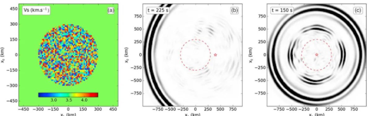
We begin with a numerical example of the interaction between an explosive point source and nearby small-scale heterogeneities. We study the wavefield propagation for two different source locations in the same 2-D elastic medium. The elastic model is built as a 600 × 600 km2_{heterogeneous matrix of 50 × 50 square}

elements, embedded in a 2400 × 2400 km2_{homogeneous square (see Figure 1), with perfectly matched}

layers (PML) [e.g., Festa et al., 2005] surrounding the physical domain to mimic radiation conditions. In each element of the heterogeneous matrix, the elastic properties are homogeneous but their values are randomly generated with a uniform distribution within ±25% of the outer square elastic values. Only one realization of the random elastic properties within the heterogeneous matrix is performed: it is therefore a deterministic medium.

For the first experiment, an explosive point source is located outside the heterogeneous inner square (100 km away) and inside for the second experiment. For both experiments, the wavefield induced by an explosive source with a Ricker wavelet time function of 50 s central period and 20 s corner period (corresponding to a 70 km minimum wavelength) is computed using the SEM with a mesh of square elements which honors all the physical discontinuities of the model.

Snapshots of the resulting seismic kinetic energy for the two cases are shown in Figure 1. It clearly appears that when the source is outside and more than one wavelength away of the heterogeneous square, only one circular coherent energy ring, typical of an explosive ballistic isotropic P wavefront, can be observed, followed by an incoherent coda wavefield. When the source is in the heterogeneous square, a second coher-ent wave front can be observed, which travels slower than the first one and has a four-lobe radiation pattern, which is typical of an S wave energy wave front generated by a double-couple source. A simple analysis (see Figure 4) shows that it is indeed the case. From these simple numerical experiments, we conclude that the existence of a second wave front (an S wave) leading to an apparent source with a double-couple component is due to the presence of heterogeneities whose size and distance to the source location are much smaller than the minimum wavelength. These heterogeneities interact with the near-field (i.e., the evanescent part of the wavefield carrying no energy, see Aki and Richards [2002, p. 85, equation 4.35]) which is dominant for dis-tances smaller than a small fraction of the minimum wavelength and can be neglected for disdis-tances greater than one or two wavelength (depending on the desired accuracy). In addition, it can be seen on Figure 2 that the four-lobe radiation pattern of the double-couple component is not generated by the propagating wave scattered by the large-scale geometrical feature of the patch of heterogeneities (i.e., the edges of the square patch in Figure 1).

In the next section, we use the homogenization theory as a tool to calculate and interpret these source-heterogeneities interactions for 2-D and 3-D cases, avoiding the complex and expensive SEM step. The 2-D experiments, allowing quick simulation, are used to first explore qualitatively the possible effects

Figure 1. (a) Heterogeneous medium represented bySwave velocity (km s−1_{). The starting values for the medium are}

PandSwave velocities of 6.1 km s−1_{and 3.57 km s}−1_{and density of 2.8 g cm}−3_{. (b) Kinetic energy snapshot (t = 225s)}

for an explosion outside of the heterogeneous square. (c) Kinetic energy snapshot (t = 150s) for an explosion inside the heterogeneous square. The represented domains are a zoom in the2400 × 2400km2actual domain, the kinetic energy is normalized, source locations are shown as red stars, and the contour of the heterogeneous square as dashed red line.

of the small-scale heterogeneities on the apparent moment tensor. The 3-D experiments, more numerically intensive, are then used to quantitatively evaluate these effects only.

3. Homogenization Principle Applied to Source-Heterogeneity Interactions

For a given heterogeneous elastic medium, a propagating wavefield with a wavelength much larger than the heterogeneity scales of the medium, only “sees” them in a effective way. In the case of a general elastic medium (that is, when no periodicity, no statistical invariance, or natural scale separation assumption can be made), the nonperiodic homogenization method [Capdeville et al., 2010a; Guillot et al., 2010; Capdeville et al., 2010b] allows the determination of an upscaled, or effective, elastic medium. Compared to many homoge-nization methods [e.g., Sanchez-Palencia, 1980; Bensoussan et al., 1978], the effective medium obtained with the nonperiodic homogenization method is, in general, not spatially uniform but is smoother than the orig-inal medium. In the forward-modeling context, this asymptotic method can be used as preprocessing stage before using a numerical wave equation solver: by removing small scales, it makes it possible to accurately model the propagation of intermediate and low-frequency wavefield at a much lower cost than when using the original medium with small-scale heterogeneities [see Capdeville et al., 2010b, 2015]. In this paper, we show that another interest of the method is to make it possible to calculate, understand, and visualize the interaction of a point source with the surrounding small-scale heterogeneities without actually solving the full elastic wave equation.

When applied to the elastodynamics issue, the nonperiodic homogenization method is based on the assump-tion that the spectrum of the considered wavefield is cutoff at a certain frequency, or equivalently, that this wavefield is defined by a minimal spatial wavelength𝜆m(which can always be the case after filtering raw

seismic data). When no specific assumption on the spatial variation of the elastic properties can be made

(that is, no periodicity, no statistical invariance, or natural scale separation) , the separation between small (microscopic) scales and large (macroscopic) scales is set by the parameter

𝜀0= 𝜆0 𝜆m

, (1)

where𝜆₀is the value below which the scales are considered as small and above which the scales are con-sidered as large.𝜀₀is user defined; it controls the degree of details that the effective model will contain with respect to𝜆_m.

In general, at any space location x and time t, the elastic displacement u(x, t) is driven by the following wave and constitutive equations

𝜌𝜕ttu −𝛁 ⋅ 𝝈 = f , (2)

𝝈 = c ∶ 𝝐 (u) , (3)

associated with appropriate initial and boundary conditions, where𝜌(x) is the medium mass density, c(x) its fourth-order elastic tensor,𝝐 (u) = 1

2

(

𝛁u +t_𝛁u)_{the strain tensor,𝝈(x, t) the stress tensor, and f(x, t) the}

seismic source vector.

The homogenization technique aims to approximate equation (2) and equation (3) with the following effective equation

𝜌𝜀0𝜕

ttu𝜀0−𝛁 ⋅ 𝝈𝜀0= f𝜀0, (4) 𝝈𝜀0_{= c}𝜀0_∶𝝐 (u𝜀0₎, ₍₅₎

where (𝜌𝜀0_(x), c𝜀0_{(x)) are the}𝜀

0effective mass density and elastic parameters, u𝜀0(x, t) is the effective

displace-ment (the order 0 homogenized displacedisplace-ment), and𝝈𝜀0_(x, t) is the effective stress (actually, the average of the

order 0 homogenized stress). As already mentioned, unlike what is usually found in many homogenization processes, the effective properties here are not spatially uniform and still depend upon the space variable x. The user defined𝜀0parameter controls the level of detail exhibited by the effective medium with respect

to𝜆m. As a consequence, all the effective quantities and solutions depend upon𝜀0. When𝜀0is small enough,

the effective displacement u𝜀0_{is a very good approximation of u (in practice, u}𝜀0_{converges towards u as}𝜀2 0).

Computing the effective medium𝜌𝜀0_{and c}𝜀0_{as well as the strain concentrator G}𝜀0_{(see below and Appendix A)}

is not a linear operation and requires to numerically solve a set of partial differential equations. The method is detailed in Capdeville et al. [2010b] and Guillot et al. [2010].

When the external source term can be described by a moment tensor M acting at x0, the external source

vector is defined as

f(x, t) = −g(t)M ⋅ 𝛁𝛿(x − x₀), (6)

where g(t) is the source time function. When there are small-scale heterogeneities near the point source, homogenization theory requires a correction of the source leading to the effective f𝜀0_{. Corrections for the}

receivers are also needed when they are embedded in small-scale heterogeneities (as it can be seen in equation (A2)), but it is a term in𝜀0which indicates it is a small effect. f𝜀0still has the same form but with an

effective moment tensor M𝜀0_{, linearly related to the original moment tensor}

M𝜀0 ≡ G𝜀0_(x

0) ∶ M, (7)

with G𝜀0_{(x), the strain concentrator (see Appendix A). Interestingly, G}𝜀0_{is a quantity that varies spatially at}

the fast scale of the small heterogeneities (that is, with details of medium, even when much smaller than the wavelength) and which, in general, does not preserve the isotropic nature of M in the explosion case. M𝜀0

is the “apparent” moment tensor and is the only one that can be retrieved with a moment tensor inversion of the low-frequency part of seismograms. Unless the heterogeneity structure around the source is perfectly known, it is not possible to recover the original moment tensor M. Nevertheless, assuming some plausible heterogeneous structures near the source, the homogenization tool can evaluate the effects of such structures on an explosion and help to interpret and understand some observed and unexpected features of related real seismic data.

Let us conclude this section by a general comment. To express the relative contributions of isotropic and deviatoric parts of the effective moment tensor, the diagonalized effective moment tensor ̄m (whose elements

̄miare the eigenvalues of M𝜀0) can be decomposed as follows:

̄m =⎡⎢ ⎢ ⎣ ̄m1 0 0 0 ̄m2 0 0 0 ̄m3 ⎤ ⎥ ⎥ ⎦ =1 3 tr(̄m) I + ⎡ ⎢ ⎢ ⎣ ̄m′ 1 0 0 0 ̄m′ 2 0 0 0 ̄m′ 3 ⎤ ⎥ ⎥ ⎦, (8)

where the isotropic moment is defined by the trace of the tensor MI=

(

̄m1+ ̄m2+ ̄m3

)

∕3 which gives access to the purely deviatoric remaining tensor (with elements ̄m′

i); this deviatoric tensor can also be decomposed

in double-couple (DC) or compensated linear vector dipole (CLVD) type of source in a nonunique way [Julian

et al., 1998]. Practically, we use the ratio pISO as the isotropic relative contribution (%), defined by Hudson et al.

[1989] as pISO = MI∕ ( |MI| + | ̄m′1| ) with| ̄m′ 1| ≥ | ̄m ′ 2| ≥ | ̄m ′

3|, and pDEV = (1 − pISO) as the deviatoric relative

contribution (%) to the moment tensor.

4. Numerical Experiments in 2-D

In this section, the interaction between a point source and local heterogeneities is qualitatively studied by per-forming 2-D numerical simulations. For a given heterogeneous elastic medium and a given corner frequency, the nonperiodic homogenization allows the calculation of the associated effective medium and correction terms for the source and receivers. As we investigate how the source is affected by local heterogeneities, the idea is to neglect the effective medium as it is small compared to the wavelength and to focus only on the effect of the source corrector as computed by the homogenization procedure.

4.1. Experiment Principle and Validation Test

In the following numerical experiments, we generate heterogeneous elastic media with various small-scale heterogeneities near the source and then compute the corresponding source correctors by using nonperiodic homogenization.

The heterogeneous medium, a 2400 × 2400 km2_{square, is designed to be homogeneous everywhere except}

in a small area around the source location (Figure 3). This small area is either composed of a single element or of a chessboard square of 2 × 2 elements (the elements are always several times smaller than𝜆m), each with

different constant elastic properties and density. These elements alternate positive and negative anomalies with respect to the homogeneous medium. For the homogeneous part of the reference medium the elastic values are those of the lower crust of the Eastern California and Western Nevada model [Song et al., 1996]:

Pand S wave velocities of 6.1 km s−1_{and 3.57 km s}−1_{and density of 2.8 g cm}−3_{(this model will be used in}

section 6 for the full moment tensor inversions). The elastic properties in the heterogeneous part are defined by their contrast with respect to the homogeneous surrounding domain.

To compute the source corrector in the heterogeneous medium, we use the 2-D finite element implemen-tation of the nonperiodic homogenization of Capdeville et al. [2010b]. To this purpose, a triangular mesh, which honors all the physical discontinuities of the model, is designed using the software Gmsh [Geuzaine and

Remacle, 2009]. The minimum wavelength of the wavefield𝜆mis chosen to be roughly equal to 70 km, which

corresponds to a cutoff period of 20 s. In general, the effective medium and source corrector are necessary to obtain an accurate effective solution. Here we will neglect the effective medium and use the fully surrounding homogeneous medium instead. As we will see below, such an approximation is fine because the heteroge-neous area is small. We define𝜆0to be equal to𝜆m(𝜀0= 1) which is of little importance as𝜀0mainly influences

the effective medium (it also affect the corrector but to a less extent) which is neglected and replaced by an homogeneous one. Additionally, as in our case𝜆minis large compared to the heterogeneity size, the choice of 𝜀0has almost no influence.

To validate our approach, we shall systematically compare reference and homogenized solutions both com-puted with SEM. The reference solution is comcom-puted for a simple explosion in the heterogeneous medium, which requires the design of a fine mesh to account for the discontinuities in the heterogeneous area. Although we can use larger elements outside the small heterogeneous area, the time step is determined by the smallest elements of this area, whose size is much smaller than the minimum propagated wavelength𝜆m.

It induces a large increase in the computational cost of the simulation. On the contrary, the homogenized solu-tion is computed in a fully homogeneous medium with a corrected source term (equasolu-tion (7)). It only requires

Figure 3. (a) Kinetic energy 2-D snapshot (t = 125s) for the reference run (explosion in a heterogeneous medium). (b) Kinetic energy 2-D snapshot (t = 125s) for the homogenized run (corrected source in a homogeneous medium). The represented domains are a zoom in the2400 × 2400km2_{actual domain, the kinetic energy is normalized, source}

locations are shown as red stars, and receivers locations are shown as red triangles. A zoom in of the 2-D medium around the source is represented for each graph (lower left corner) by theV_Sparameter (km/s).

a sparse mesh whose grid spacing is constrained by the minimum wavelength𝜆mas the effective medium is

neglected (or𝜆0if the effective medium is considered). In both cases, PML encircle the physical domain, and

the source time function is a Ricker wavelet with a 20 s corner period.

In order to show the simplicity and accuracy of our procedure, we present an example case for one heteroge-neous medium. The 12 × 12 km2_{heterogeneous part of the medium is composed of 2 × 2 square elements}

(6 × 6 km2_{for each element, which is more than 10 times smaller than𝜆}

m) with a contrast of elastic values

(according to Lamé parameters) and density between nearby elements of 50% (±25% between elements and the surrounding homogeneous medium). The reference medium is homogenized, and the source corrector is computed for a point source located at xs=t(720 m, 421 m), with x =t(0, 0) as the center of the heterogeneous

area. The source location has been deliberately chosen slightly off the square centre where the source correc-tion is the smallest. The relevant source correccorrec-tion is applied to an isotropic moment tensor (equacorrec-tion (7)) to obtain the corrected, effective source, which leads to a relative contribution of the deviatoric moment pDEV up to 12.3%.

Figure 3 shows two snapshots of the wavefield kinetic energy at time t = 150 s for the two cases. Similarly, as observed in Figure 1, two coherent wavefronts arise in the reference solution; the first is the expected P wave front and the slower second one is typical of an S wave front induced by a double-couple source mechanism, which is the only deviatoric source type possible in the 2-D case. This strong S wave front is not generated by any far-field propagation effect but by the interaction between the near-field and small-scale heterogeneities located in the immediate vicinity of the source. The heterogeneities can be small for their spatial extension and still interact with the source and create this strong S wave coherent front (if the elastic contrast is large enough). On the homogenized solution snapshot, it clearly appears that the wavefield, generated by the cor-rected source and in the absence of any heterogeneities near the source, accurately reproduces the reference one (including the S wave front).

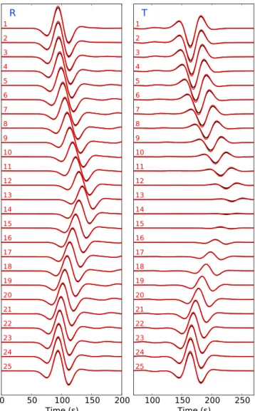
In Figure 4 are reported the seismograms recorded at the receivers locations (plotted in Figure 3). It can be seen that the reference (u) and homogenized (u𝜀0_{) solutions are in good agreement for both radial and transverse}

components. Using displacement L2_{norm misfit𝜉 =}√_∫tmax

0 (u𝜀0− u)2(t)dt ∕

√ ∫tmax

0 u2(t)dt, for instance, we

obtain at the 23rd receiver𝜉 = 0.062 for the radial component and 𝜉 = 0.076 for the transverse component. These small remaining differences are due to the fact that the true effective medium has been replaced by a purely homogeneous medium.

This simple numerical example validates our procedure and emphasizes the near-field nature of this process. The strong S wave front is due to the heterogeneities in the immediate vicinity of the source; hence, a large complex medium as shown in Figure 1 or 2 is not necessary, 2×2 heterogeneities (Figure 3), or even one single heterogeneity (Figure B1) at the source is enough.

Figure 4. (left) Radial and (right) transverse components of displacement recorded at the receivers shown in Figure 3.

The reference solution is plotted in black and the corrected source solution is plotted in red.

Moreover, this canonical example of a 12 km heterogeneous area which is much smaller than the 70 km min-imum wavelength associated with the 20 s corner period of the source, is scalable to, for example, a 120 m heterogeneous area with a 5 Hz corner frequency (corresponding to a 700 m minimum wavelength), which will produce the exact same result.

4.2. Effect of the Heterogeneity Relative Amplitude

First, we consider how much the source corrector depends on the strength (i.e., the amplitude of the pertur-bation of elastic values relatively to the homogeneous background medium) of the anomalies located in the small heterogeneous area. To that purpose, we use the same mesh as the one in the validation test, a 12 × 12 km2_{wide area of 2 × 2 heterogeneous square elements around the source (the elements are more than 10}

times smaller than𝜆m). We then generate a series of perturbed elastic values and density ranging from 5% to

150% between nearby elements (corresponding to the range ±2.5% to ±75% between the elements and the surrounding homogeneous medium). Such heterogeneity contrasts are large but not unrealistic, especially in the shallower layers of the Earth and at small scales.

All of these heterogeneous models are subsequently homogenized using nonperiodic homogenization at order 0, and for each model, the source corrector G𝜀0₍̂x) is computed on a 2-D grid sampling ̂x of the part of

the domain around the area of heterogeneities (̂x ∈ [−12 km, 12 km]2_).

Figure 5 shows, for some values of the heterogeneity strength, the distribution of the relative contribution of the deviatoric moment pDEV(̂x), associated with corrected moment tensor (equation (7)) for each sample

Figure 5. Deviatoric componentpDEV distribution for three 2-D heterogeneous media with various amplitude contrast values: (a) 20%, (b) 50%, and (c) 80%. Focal mechanisms of the deviatoric component are shown for some specific source locations on Figure 5.

of the heterogeneous area. This illustrates how strongly the source signature is perturbed as a function of its location within the area of heterogeneities. Obviously, the pDEV(̂x) values increase as the amplitude of the elastic and density anomalies increases throughout the heterogeneous area, for example, at x =t_{(1.2 km,}

1.8 km): we find pDEV(20%) = 4.2%, pDEV(50%) = 9.4%, and pDEV(80%) = 13.4%. Moreover, we can notice throughout the distribution of pDEV that the strongest values are confined to regions with the largest velocity variations.

The maximum value of pDEV(̂x) (within the heterogeneous area) is picked out for the full range of amplitude perturbations (Figure 10). It seems to increase logarithmically, reaching, respectively, 18%, 29%, and 39% for 20%, 40%, and 80% elastic values and density perturbations.

4.3. Effect of Heterogeneity Size and Position

Second, we consider the influence of the heterogeneity size on the source corrector, as well as the effect of its relative location with respect to the point source. To that end, we generate heterogeneous models containing a single quadrangle heterogeneous area whose size is varying from 2 × 2 km2_{to 20 × 20 km}2_{. The elastic}

values and density perturbation with the surrounding medium is identical for all the models (50%).

Each heterogeneity model is homogenized using nonperiodic homogenization at order 0. For each model, the source corrector is computed for a line of source locations starting from the interface between the het-erogeneous quadrangle and the homogeneous surrounding medium to 500 km away from the quadrangle (for distance much smaller than𝜆_mto much greater than𝜆_m).

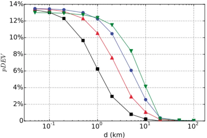
Figure 6. Deviatoric componentpDEV associated with the corrected tensor as a function of the size and the distance (d) to a single 2-D square heterogeneity (of 50% elastic contrast). The deviatoric component evolution is represented for different heterogeneity size:2 × 2km2_(black),

5 × 5km2_{(red),10 × 10km}2_{(blue), and20 × 20km}2_(green).

Figure 6 shows, for some heterogene-ity size values, the relative contribu-tion of the deviatoric moment pDEV (for a corrected isotropic moment tensor) as a function of the distance to the heterogeneity. Regardless of the heterogeneity size, pDEV decreases in a sigmoid-shaped way as a function of the logarithm of the distance. It appears that the smaller the hetero-geneity is, the faster pDEV decreases. For instance, pDEV reaches half of its maximum value at 1.1 km distance for a 2 km heterogeneity, while it reaches the same value at 2.8 km, 5.1 km, and 7.4 km for a 5 km, 10 km, and 20 km heterogeneity, respectively. Another point is that independently of the het-erogeneity size, pDEV strongly tends

to zero for a source-heterogeneity distance greater than 20 km, which has to be related to the identical mini-mum wavelength𝜆_m= 70 km (corresponding to a 20 s minimum period) used for the homogenization of all heterogeneous models.

5. Numerical Experiments in 3-D

We now keep analyzing the interaction between point source and local heterogeneities but in the 3-D case. As in the previous section, we use nonperiodic homogenization to compute the source corrector (and neglect the effective medium) associated with some models containing near-source small-scale heterogeneities.

5.1. Experiment Principle and Validation Test

The 3-D heterogeneous medium is a 1200 × 1200 × 1200 km3_{cube, which is designed to be homogeneous}

except in one near-source small area (compared to the minimum wavelength𝜆m) of heterogeneities. The

small heterogeneous area is a 12 × 12 × 12 km3_{chessboard cube of 2 × 2 × 2 elements, each with constant}

elastic properties and density. These eight elements alternate positive and negative perturbations relatively to the homogeneous surrounding medium. The elastic values and density of the homogeneous medium and the heterogeneous elements are the same as that described in section 4.1.

The computation of the source corrector for a heterogeneous medium is performed using the 3-D implemen-tation of the nonperiodic homogenization at order 0 of Capdeville et al. [2015]. Unlike the 2-D implemenimplemen-tation used in section 4 which is adapted to discontinuous media, this 3-D implementation extensively relies on a fast Fourier transform iterative algorithm that implies a regular gridding of the medium which is more adapted to continuous media. Thus, we could expect some numerical difficulties in our case, because of the small-scale heterogeneities and discontinuities in the model. Nevertheless, this problem will be addressed further in the section and found not to be really an issue. As in section 4 the minimum period in the wavefield is 20 s, cor-responding to a minimum wavelength𝜆m= 70 km. Once again, the (small) lateral variations of the effective

medium are neglected to only keep the source corrector, we use a𝜀0equal to 1.

The heterogeneous initial model contains interfaces and since the homogenization requires a continuous sampling, we reach the smallest possible sampling of 25 m (for 6 km wide heterogeneous elements) using extensive parallel computing resource to obtain the more accurate possible homogenized solution. This sampling step corresponds to a 3 × 103_{factor compared to the minimum propagated wavelength𝜆}

m.

Once again, the accuracy of this approach can be evaluated using a 3-D SEM solver for computing reference and homogenized solutions. As in section 4, the reference solution is obtained using SEM in the fine-scale medium. Such a computation is CPU demanding, due to the occurrence of small-scale elements, requiring a fine hexahedral mesh, hence a small time step. Computing the homogenized solution only requires a sparse mesh for the homogeneous medium and a corrected source (equation (7)) and is as usual much a cheaper task than for the reference solution. For both meshes the physical medium is surrounded by PMLs, and the source time function is a Ricker wavelet of 20 s corner period.

To assess the accuracy of our 3-D procedure, we present a 3-D example case which is similar to the 2-D exam-ple case shown in section 4.1. The heterogeneous model is homogenized, the effective medium is neglected and replaced by an homogeneous medium, and the source corrector is computed for a source located at

x_s=t_{(600 m, −2040 m, 600 m), with x =}t_{(0, 0, 0) the center of the heterogeneous area). The corrected source}

is obtained by applying the source corrector to an isotropic moment tensor, showing a relative contribution of the deviatoric moment tensor pDEV roughly equal to 24.3%. We use a 3-D SEM solver to compute the ref-erence solution (explosion in the heterogeneous medium) and the homogenized solution (corrected source in a homogeneous medium) for the same configuration of source and receivers locations.

Snapshots of the two resulting wavefields are shown in Figure 7 at time t = 125 s. As in 2-D, two coherent wavefronts can be observed, the faster one is the P wave front and the slower one is an S wave radiation pat-tern (SV and SH wave energy). This S wave energy front is generated by the interaction of the compressional wavefield with the small-scale heterogeneities near the explosive point source. The homogenized solution presents almost identical wavefield characteristics, which implies that the corrected source accurately inte-grates the effect of the near-source heterogeneities. It should be emphasized that this source can produce either DC or CLVD as a function of its location in the heterogeneous area (see Appendix B for a preliminary analysis of the corrected source decomposition into DC/CLVD in the 3-D case).

Figure 7. (a) Kinetic energy 3-D snapshot (t = 125s) for the reference run (explosion in a heterogeneous medium). (b) Kinetic energy 3-D snapshot (t = 125s) for the homogenized run (corrected source in a homogeneous medium). The kinetic energy is normalized, source locations are shown as a blue dots, and receiver locations are shown as red dots. The 3-D medium around the source is represented for each graph (lower left corner) by theVSparameter (km/s).

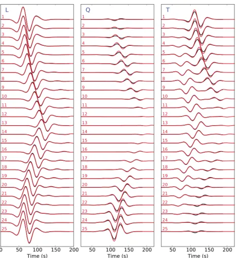
We also show the three-component seismograms recorded at the receivers locations for both reference and homogenized cases in Figure 8. P wave direction component (L) shows a good agreement between reference and homogenized solutions, while SV wave (Q) and SH wave (T) directions components present lower but satisfactory agreement in amplitude. For example, at the 25th receiver, the displacement L2_{norm misfit𝜉 is}

Figure 8.Pwave direction (L, left),SVwave direction (Q, center), andSHwave direction (T, right) components of the displacement recorded at the receivers shown in Figure 7. The reference solution is plotted in black, and the corrected source solution is plotted in red.

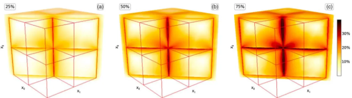
Figure 9. Deviatoric componentpDEV distribution for three 3-D heterogeneous media with various amplitude contrast values: (a) 25%, (b) 50%, and (c) 75%.

equal to 0.04 for the L component and 0.24 for the Q component and at the second receiver,𝜉 is equal to 0.04 for the L component and 0.27 for the T component. These remaining small differences can be due to the inadequate sampling of our discontinuous heterogeneous medium for the nonperiodic homogenization procedure and also to the fact that we neglect the effective medium in the source area and propagate the wavefield in a purely homogeneous medium.

5.2. Effect of the Heterogeneity Relative Amplitude

For the 3-D case, we only consider the effect of near-source anomalies amplitude on the source corrector. For that purpose, we generate a series of perturbed elastic values and density ranging from 5% to 140% between nearby elements inside the heterogeneous area (corresponding to the range ±2.5% to ±70% between the elements and the surrounding medium).

We apply 3-D nonperiodic homogenization on these heterogeneous models and compute the source correc-tor distribution G𝜀0₍̂x) for a 3-D grid sampling of the heterogeneous area ̂x ∈ [−12 km, 12 km]3_.

The distribution of the relative contribution of the deviatoric moment pDEV(̂x) (associated with the source corrector distribution for an isotropic tensor) is shown in Figure 9 for some amplitude values. As expected, larger-amplitude anomalies produced stronger pDEV for the whole heterogeneous area. At point

x =t_{(2.88 km, 1.68 km, −0.24 km), we find pDEV(25%) = 13.2%, pDEV(50%) = 21.4%, and pDEV(75%) = 26.7%.}

Besides, it appears that pDEV stronger values are located at the junction of the elements (vertices, faces, and edges) and also in lobes along the edges.

The maximum values of pDEV(̂x) for the entire series of heterogeneous models are also reported in Figure 10. It shows a similar trend but a larger increase than the 2-D results, reaching 23%, 37%, and 51% for 20%, 40%, and 80% elastic values and density perturbations, respectively.

Figure 10. Maximum deviatoric componentpDEV for a series of heterogeneous media with amplitude contrast values ranging from 5% to 135%. The evolution of maximum deviatoric component is shown for the 3-D simulations (black) and the 2-D simulations (grey).

6. Deviatoric Moment

From Explosion Data

The aim of this section is to assess if the numerically observed effects of small-scale heterogeneities on moment tensors (see sections 4 and 5) are compatible with what can be measured on long period data from underground explosions. Such data are very well suited to achieve our goal for the following reasons: (1) the original unaffected moment tensor for an explosion is a priori known; (2) the minimum wavelength of the wavefield is much larger than the characte-ristic size of the geological hetero-geneities around the point source;

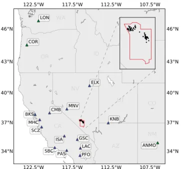
Figure 11. Map of the western United States. Stations (blue triangles) and events (black circles) used in this study

are shown. All the events are located within the boundaries of the Nevada Test Site (red). A blowup of the events distribution is shown on the top right corner.

(3) neglecting 3-D wave propagation effects is less critical than at short period; (4) finally because of the recurrence of nuclear shots in the same, small areas it is easier to find different sources within a distance small compared to the wavelength for explosion experiments than for any other type of sources.

We select the well-known database of the U.S. nuclear tests conducted at the Nevada National Security Site (NNSS, formerly known as the Nevada Test Site) until 1992 for which the date, time, yield, location, and depth of burial of events are directly available [Springer et al., 2002]. We collect three-component data from all the regional broadband stations available for the largest NNSS nuclear tests since the year 1980 (about 80 events). We only keep the data which present a high signal-to-noise ratio in order to obtain a total of 42 events (from Pahute Mesa and Yucca Flat regions) recorded at 14 stations from the TriNet, Incorporated Research Institutions for Seismology/U.S. Geological Survey, Berkeley Digital Seismic Network, the Lawrence Livermore National Laboratory (LLNL) network, and Geoscope networks (Figure 11). Most of the stations are located between azimuth 180∘ and 310∘ with epicentral distance from 1.8∘ to 4.7∘, except three stations approxi-mately at 10∘. We remove the instrument response and filter the data between 20 s and 50 s (except for the LLNL stations, for which we use the period range 10 s–30 s due to inaccurate sensitivity of instruments at long period).

First, data are analyzed by comparing events whose detonation points are located within a very close distance to each others such that observed differences in the waveforms can only be related to phenomena occurring right at the source. Second, multiple events are gathered and compared at the same station in a more sys-tematic manner. Third, we perform a full moment tensor inversion for some NNSS events in order to obtain the effective moment tensor, whose deviatoric contribution is a measurement of the observed nonisotropic radiation. It establishes reference values for comparison with our numerical experiments.

6.1. Nearby Events

As the NNSS database contains a large number of closely located events, we can study the occurrence of nonisotropic radiation by comparing pairs of very close events. Thus, the possible propagation effects can be neglected: the distance between a pair of events is small enough with respect to the wavelength of the wavefield; waves are considered to propagate along similar paths. It implies that anomalous perturbations in the waveforms between the pair of events are related to a near-source phenomenon only.

All possible combinations of pairs among the 42 selected events have been tested; we find interdistances between events ranging from 600 m up to 50 km. There is a large number of pairs of events whose inter-distance is much smaller than the minimum wavelength of the wavefield (roughly equal to 70 km here).

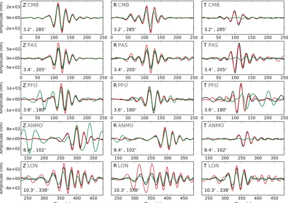
Figure 12. Three components data from common stations for events MONTELLO (black), HOYA (red), and COMSTOCK

(green). Vertical (Z), radial (R), and transverse (T) components are filtered between 20 and 50 s. On the lower left corner of each vertical plot, the epicentral distance, and azimuth are indicated.

However, to be compared, both events must also have approximately the same magnitude and be recorded at a number of common stations which is large enough.

We select two pairs of events from the Pahute Mesa area which satisfy these criteria: MONTELLO/HOYA and MONTELLO/COMSTOCK. The depths of burial of the events are almost equal, for MONTELLO, HOYA, and COMSTOCK they are 658 m, 642 m, and 620 m, respectively. The distance between events MONTELLO and HOYA is 2.5 km and 1.7 km between MONTELLO and COMSTOCK (Figure 12). These interdistances are much smaller than the smallest wavelength of the wavefield. We can see in Figure 12 that the waveforms of the couple of events MONTELLO/HOYA present a pretty good agreement for the three components at all com-mon stations (except for the radial component of the most distant station LON), notably for the transverse components which show large amplitudes, almost of the same order as the radial and vertical components. For the couple of events MONTELLO/COMSTOCK (Figure 12) we can notice that while there is a good agree-ment between radial and vertical components, the amplitude of the transverse components associated with the event MONTELLO is much larger than the ones associated with the event COMSTOCK (except for the station LON), which is very small with respect to the radial and vertical components.

In the first case (MONTELLO/HOYA) we observe the same high amplitudes for the transverse components (and more generally, quite similar waveforms) for events separated by a distance of 2.5 km, the sources of the two events could have interacted with the local heterogeneities in the same way. However, one has to consider that source-receiver path effects may also lead to the occurrence of large tangential components. In the second case (MONTELLO/COMSTOCK) we observe a large discrepancy between seismograms associated with the two events. This seems to indicate that the phenomenon leading to a nonzero amplitude transverse component is located near the source and that local heterogeneities< 1.7 km wide may dramatically affect the regional waveforms (see section 7).

6.2. Station Collection

Another approach to analyze the data and point out the nonisotropic radiation effects in the observations, and similar to that of the previous section, is to compare all events that have been recorded at the same station.

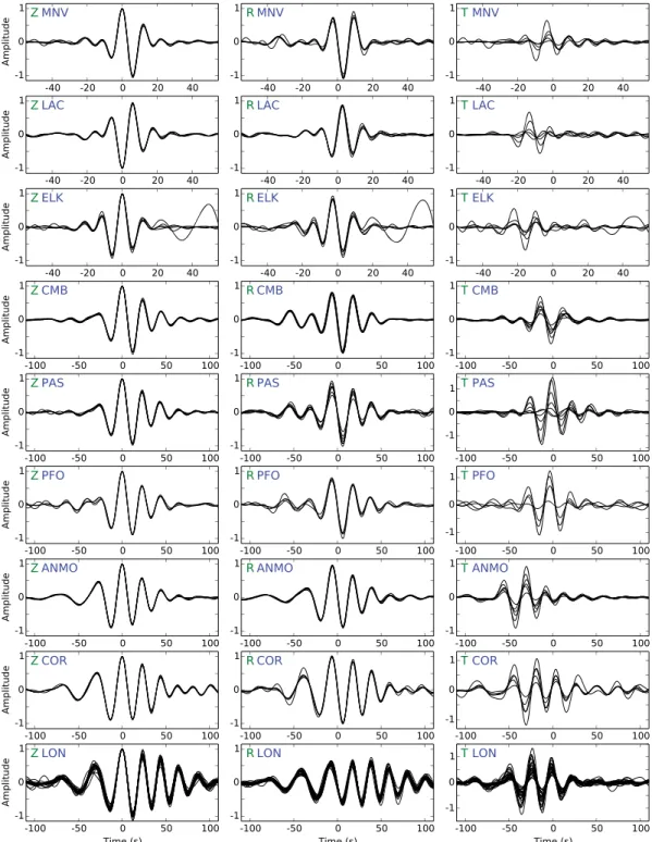
Figure 13. Multiple events at same stations. For all the events recorded at each station, the amplitude of the three

components are normalized to the maximum amplitude of the vertical component. The data are filtered between 20 and 50 s except for the LLNL stations (MNV, LAC, and ELK) which are filtered between 10 and 30 s. On the lower left corner of each vertical plot, the epicentral distance and azimuth are indicated. The scale of the transverse component may be larger than the others.

We select the stations that recorded a large number of events, with a high signal-to-noise ratio for the three components. Moreover, we limit the interdistance between events to a maximum value of 10 km which is much smaller than the minimum wavelength caught in the filtered data (70 km) even for the LLNL stations (35 km for a minimum period of 10 s). In order to compare different events with different magnitudes, we shift and normalize the three components, respectively, by the time and largest value of the vertical component for each event.

In Figure 13 are shown eight stations that have recorded enough events with a high signal-to-noise ratio (5 to 7 depending on the stations). These stations present a wide range of epicentral distance (1.8∘ to 10.4∘) and azimuthal coverage at the regional scale. The LLNL stations (MNV, LAC, and ELK), which are filtered in a narrower frequency band, present an accurate match of the vertical and radial waveforms for the multiple events, whereas the waveforms for the transverse component show various amplitudes and some phase shifts for the different events. The maximum amplitudes are 50% less than the vertical one. The longer-period sta-tions (CMB, PAS, ANMO, and COR) also present an accurate match for the vertical and radial components, while the waveforms of the transverse component show diverse amplitudes, with maximum values in the order of the vertical one except for the station PAS, where maximum amplitudes are 50% more than the vertical component. At the bottom of Figure 13 are shown seismograms recorded at the station LON: they present the largest number of records (26 events). Once again, the transverse component waveforms present a range from low to very high amplitudes.

We notice a large range of amplitudes on the transverse component depending on the events, indeed with small distance between events compared to the wavelength, a large effect on the transverse component amplitude is observed, which could be related to a local interaction with the source. Additionally, the dif-ference between LLNL stations and longer-period stations could be an indication on the size of the local heterogeneities. Indeed, the interaction between the near-field and small-scale heterogeneities located in the vicinity of the source requires that the minimum wavelength of the wavefield is much larger than the size of heterogeneities. As soon as the frequency increases, the minimum wavelength decreases and the size of heterogeneities can no longer be seen as small scales.

6.3. Moment Tensor Inversion

We now consider the quantification of the nonisotropic radiation for a selection of NNSS events. A classical representation of the properties of a point source is the full seismic moment tensor [Gilbert, 1971]. In the case of a pure explosion, the moment tensor is isotropic (only related to volume variation). Otherwise, any nonisotropic radiation implies a deviatoric part in its moment tensor representation. Therefore, the moment tensor inversion of a carefully chosen data set provides a measure of the deviatoric parts that can be compared to results of sections 4 and 5.

We invert for the moment tensors of 11 NNSS events, which are selected according to the number of stations available for each event (four at least) and the quality of the signal-to-noise ratio on the three components. We implement a time domain inversion of the data for the full moment tensor; this data vector is made of the time seismograms u of all their components at all stations available; in vectorial form, d = t(_u

1, … , uk, …

) , where u_kis the displacement associated to the kth data. Seismograms can be expressed as linear combina-tions of components of the moment tensor and the associated Green’s funccombina-tions [Stump and Johnson, 1977]. The synthetic displacement̄u_kassociated with the kth data is related to m_i, the ith component of the moment tensor and G_kithe associated Green’s function, as

̄uk(x, t) = ∑ i Gki(x, t) mi (9) or in matrix form ̄u = G ⋅ m , (10)

where m is a vector gathering the six independent components of the moment tensor and G the correspond-ing Green’s functions. As we are able to build the Green’s function (we know the location and depth of the explosions) in equation (10), following Tarantola and Valette [1982], it is simple to solve the least square inverse problem minimizing the L2_{misfit between data u and synthetic seismograms ̄u to obtain the estimated}

moment tensor components:

Figure 14. Three-component data (black) and synthetics (red) associated to the best fitting moment tensor solution for

the event BEXAR. The data are filtered between 20 and 50 s except for the LLNL stations (KNB and LAC) which are filtered between 10 and 30 s. On the lower left corner of each vertical plot, the epicentral distance and azimuth are indicated.

In order to have a better constraint of the isotropic part of the full moment tensor, the moment tensor is decomposed into a combination of elementary sources, as

m_i=∑

n

a_nm∗

in, (12)

where m∗

inis the ith component of the nth elementary source and anits associated coefficient. Then we can

rewrite equation (9) with equation (12) as

uk(x, t) = ∑ n G∗ kn(x, t) an, (13) where G∗

knare the Green’s function associated with the elementary sources. We choose to use the

decompo-sition of Kikuchi and Kanamori [1991], based on elementary sources

M∗ 1,…,6= ⎡ ⎢ ⎢ ⎣ 0 1 0 1 0 0 0 0 0 ⎤ ⎥ ⎥ ⎦, ⎡ ⎢ ⎢ ⎣ 1 0 0 0 −1 0 0 0 0 ⎤ ⎥ ⎥ ⎦, ⎡ ⎢ ⎢ ⎣ 0 0 0 0 0 1 0 1 0 ⎤ ⎥ ⎥ ⎦, ⎡ ⎢ ⎢ ⎣ 0 0 1 0 0 0 1 0 0 ⎤ ⎥ ⎥ ⎦, ⎡ ⎢ ⎢ ⎣ −1 0 0 0 0 0 0 0 1 ⎤ ⎥ ⎥ ⎦, ⎡ ⎢ ⎢ ⎣ 1 0 0 0 1 0 0 0 1 ⎤ ⎥ ⎥ ⎦.

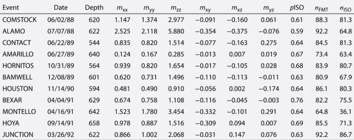
Table 1. Summary of the Full Moment Tensor Inversion Resultsa

Event Date Depth m_xx m_yy m_zz m_xy m_xz m_yz pISO _{𝜎FMT 𝜎ISO} COMSTOCK 06/02/88 620 1.147 1.374 2.977 −0.091 −0.160 0.061 0.61 88.3 81.3 ALAMO 07/07/88 622 2.525 2.118 5.880 −0.354 −0.375 −0.076 0.59 92.2 64.8 CONTACT 06/22/89 544 0.835 0.820 1.514 −0.077 −0.163 0.275 0.64 84.5 81.3 AMARILLO 06/27/89 640 0.124 0.167 0.285 −0.013 0.007 0.019 0.67 73.4 63.4 HORNITOS 10/31/89 564 0.939 0.820 1.654 −0.017 −0.105 0.028 0.68 83.9 80.7 BAMWELL 12/08/89 601 0.620 0.731 1.496 −0.110 −0.113 −0.011 0.63 80.9 67.9 HOUSTON 11/14/90 594 0.481 0.490 0.910 −0.056 0.002 −0.174 0.64 86.1 80.3 BEXAR 04/04/91 629 0.674 0.758 1.108 −0.116 −0.045 −0.003 0.76 82.2 75.5 MONTELLO 04/16/91 642 1.523 1.780 3.454 −0.332 −0.101 0.291 0.64 64.8 36.1 HOYA 09/14/91 658 0.978 0.887 1.516 −0.309 0.094 0.007 0.69 85.5 71.3 JUNCTION 03/26/92 622 0.866 1.002 2.068 −0.031 0.147 0.076 0.63 92.2 86.7

a_{The depths of burial of the events are in meters. The Cartesian tensor components are in10}16_{N m. The variance}

reductions for full moment tensor inversion_𝜎FMTand explosive source_𝜎ISOare in percent.

Thus, the components of the full moment tensor are retrieved from the coefficients of the elementary sources, and we can rewrite equation (12) as

M = ⎡ ⎢ ⎢ ⎣ m₁ m₄ m₅ m₄ m₂ m₆ m₅ m₆ m₃ ⎤ ⎥ ⎥ ⎦ = ⎡ ⎢ ⎢ ⎣ a₂− a₅+ a₆ a₁ a₄ a₁ −a₂+ a₆ a₃ a₄ a₃ a₅+ a₆ ⎤ ⎥ ⎥ ⎦. (14)

The computation of the Green’s functions is based on a 1-D elastic model of Eastern California and Western Nevada [Song et al., 1996]. To address uncertainties in the elastic model, following Ford et al. [2009], we first compute a population of models by the perturbation of model parameters (for each parameter of the model, three specific values are possible). Second, in the inversion process, the Green’s function are allowed to shift with respect to the data (shifts are small compared to the period). The Green’s functions are calculated for each model and each elementary source by using the normal modes method. The inversion of data for the full moment tensor (equation (11)) is performed for the 11 selected events and for the whole population of models. We keep the models and shifts which show the best fit to the data, with the fit𝜎 (variance reduction) defined as 𝜎 = ⎛ ⎜ ⎜ ⎜ ⎝ 1 − ∑ k √ ∫tmax 0 (̄uk− uk)2(t)dt ∑ k √ ∫tmax 0 u2k(t)dt ⎞ ⎟ ⎟ ⎟ ⎠ . (15)

As an example, we show data and synthetics waveforms resulting of the full moment tensor inversion for the event BEXAR in Figure 14. Despite small-amplitude overestimations (stations PAS and PFO) for the vertical and radial components, the data and synthetics are in good agreement.

All the results of the full moment tensor inversion for the 11 NNSS events are summarized in Table 1. We find moment tensor solutions with high variance reduction>80% except for MONTELLO and AMARILLO and even

>90% for some events (ALAMO, JUNCTION). The improvement of the variance reduction compared to a purely

isotropic source range from 3% to 29% depending on the amplitudes of the transverse components for the event. The magnitude of the variance reduction depends on how different is the source from a pure explosion and, in our case, how strong is the transverse component. In the case of a strong transverse component the variance reduction between isotropic solution and full moment tensor solution will be large, but with a weak transverse component it could be small.

We find isotropic moment contributions pISO ranging from 59% to 76%, with an average of about 65%. Our results are in good agreement with the study of Ford et al. [2009] (which take into account a larger number of events and with a refined method). Ford et al. [2009] find average pISO values about 64%, with maximum values at 79%.

7. Discussion

The present work is a first attempt to show that the elastic interaction between local small-scale hetero-geneities (or a single heterogeneity) and a point source is a phenomenon that is efficient in perturbing the initial radiation pattern. The homogenization theory, and its application to the source term, appears to be an accurate and convenient technique to understand and calculate these local interactions. It allows us to go further as what can be obtained using the perturbative approach suggested by Leavy [1993], as far as the heterogeneity size is much smaller than the smallest wavelength of the wavefield.

Moment tensor inversions for carefully chosen NNSS events seem to indicate that the level of anisotropy in their effective radiation (an average of 35%) is somewhat larger than what can be generally obtained in the 2-D and 3-D numerical experiments conducted previously in this paper. According to these experiments, these high values can nevertheless be reached with the following configurations: a moderate amplitude heterogeneity in the immediate vicinity of the source or a more distant one but with a stronger amplitude. In this systematic study, we use hypothetical values for the contrast of elastic parameters and density, ranging from 5% to 145%, as well as for heterogeneity dimensions, down to 6 × 6 × 6 km3_{. As an example, we can}

compare our values with the NNSS area geological settings [Howard, 1985]. Among the four main geological units that can be distinguished (sedimentary deposits, volcanic tuff, carbonate rocks, and plutonic rocks), we observe elastic contrasts ranging from 72% to 150% and these units are several kilometers wide and several hundreds of meters deep. Thus, our hypothetical values are reasonable and more extreme properties for the heterogeneity size in particular (much smaller features) can be found. Moreover, realistic geology could also involve anisotropy, solid-fluid interface and complex geometry which we have not investigated yet. An important application is related to the effective radiation associated with an explosive point source. We want to underline that the elastic source/small heterogeneities interactions should not be ruled out, concerning the generation of anomalous S wave observed in the low-frequency part of seismograms, as has often been the case [Massé, 1981; Patton, 1991]. As pointed by Leavy [1993], the first and main effect related to the occurrence of small scatterers in the near-field is the generation of a scattered field with a quadrantal pattern and primary waves similar to those associated with an earthquake and therefore SH-polarized waves (it should be noted that this polarization is defined with respect to the coordinate system related to this “earthquake” double-couple). This mechanism may explain an intriguing observation: Rayleigh wave signals related to explosions at the same test site are similar (in the time and frequency domains) at a given station and do not change as the number of shots grow [McEvilly and Peppin, 1972].

This fact seemed to rule out the tectonic release hypothesis [Massé, 1981], as these signals should be lowered after a detonation. On the contrary, our hypothesis does not contradict this observation as the amplitudes of the initial and scattered fields are linearly related (equation (7)) and not distorted by any real tectonic component. This observation is particularly interesting and should be accounted for in the scaling of the long-period explosion spectrum or in yield estimation. Finally, one ought to notice that depending on the rel-ative geographical position of the couple source/heterogeneities, the characteristics of the earthquake-like component may be those of a strike-slip, a dip-slip, or a CLVD source mechanisms, which is the same as the ones classically mentioned when considering tectonic release or block-driven motions, respectively, to explain anomalous generation of S components for explosive sources.

8. Conclusion and Perspectives

We have studied the macroscopic interaction of point sources with nearby heterogeneities of size much smaller than the wavelength. Our work is based on the nonperiodic homogenization method which makes possible to perform such a study without explicitly computing synthetic seismograms in complex models and to obtain directly the effective moment tensor accounting for the small-scale point source interaction. We have conducted a set of 2-D and 3-D numerical experiments based on this method which have been validated against a reference solution computed using the SEM solver. On one hand, the application of non-periodic homogenization to reference media with small-scale heterogeneities around the source gives access to the effective moment tensor and the associated deviatoric contribution to the seismic moment. This study shows deviatoric contributions reaching 21% for 2-D and 27% for 3-D near-source heterogeneities presenting a 25% contrast of elastic values.