Y-shaped jets driven by an ultrasonic beam reflecting on a wall

HAL Id: hal-01174278

https://hal.archives-ouvertes.fr/hal-01174278

Submitted on 8 Jul 2015

HAL is a multi-disciplinary open access

archive for the deposit and dissemination of sci-entific research documents, whether they are pub-lished or not. The documents may come from teaching and research institutions in France or abroad, or from public or private research centers.

L’archive ouverte pluridisciplinaire HAL, est destinée au dépôt et à la diffusion de documents scientifiques de niveau recherche, publiés ou non, émanant des établissements d’enseignement et de recherche français ou étrangers, des laboratoires publics ou privés.

Y-shaped jets driven by an ultrasonic beam reflecting on

a wall

Brahim Moudjed, Valéry Botton, Daniel Henry, Séverine Millet, Hamda Ben

Hadid

To cite this version:

Brahim Moudjed, Valéry Botton, Daniel Henry, Séverine Millet, Hamda Ben Hadid. Y-shaped

jets driven by an ultrasonic beam reflecting on a wall. Ultrasonics, Elsevier, 2016, 68, pp.33-42. �10.1016/j.ultras.2016.02.003�. �hal-01174278�

1

Y-shaped jets driven by an ultrasonic beam reflecting

on a wall.

Brahim Moudjed

, Valéry Botton

, Daniel Henry

, Séverine Millet

, and Hamda Ben Hadid

1

Laboratoire de Mécanique des Fluides et d’Acoustique, CNRS/Université de Lyon,

Ecole Centrale de Lyon/Université Lyon 1/INSA de Lyon,

ECL, 36 avenue Guy de Collongue, 69134 Ecully Cedex, France

2

CEA, Laboratoire d’Instrumentation et d’Expérimentation en Mécanique des Fluides et

Thermohydraulique, DEN/DANS/DM2S/STMF/LIEFT, CEA-Saclay, F-91191 Gif-sur-Yvette

Cedex, France

Abstract

This paper presents an original experimental and numerical investigation of acoustic

streaming driven by an acoustic beam reflecting on a wall. The water experiment features a 2

MHz acoustic beam totally reflecting on one of the tank glass walls. The velocity field in the

plane containing the incident and reflected beam axes is investigated using Particle Image

Velocimetry (PIV). It exhibits an original y-shaped structure: the impinging jet driven by the

incident beam is continued by a wall jet, and a second jet is driven by the reflected beam,

making an angle with the impinging jet. The flow is also numerically modeled as that of an

incompressible fluid undergoing a volumetric acoustic force. This is a classical approach, but

the complexity of the acoustic field in the reflection zone, however, makes it difficult to

derive an exact force field in this area. Several approximations are thus tested; we show that

the observed velocity field only weakly depends on the approximation used in this small

region. The numerical model results are in good agreement with the experimental results. The

spreading of the jets around their impingement points and the creeping of the wall jets along

the walls are observed to allow the interaction of the flow with a large wall surface, which can

even extend to the corners of the tank; this could be an interesting feature for applications

requiring efficient heat and mass transfer at the wall. More fundamentally, the velocity field is

shown to have both similarities and differences with the velocity field in a classical centered

acoustic streaming jet. In particular its magnitude exhibits a fairly good agreement with a

formerly derived scaling law based on the balance of the acoustic forcing with the inertia due

to the flow acceleration along the beam axis.

Keywords : acoustic streaming, steady streaming, reflections, jets, Eckart.

1. Introduction

Acoustic streaming designates the ability to drive quasi-steady flows by acoustic propagation in dissipative fluids and results from an acousto-hydrodynamics coupling. Nyborg [1] and Lighthill [2] gave a theoretical insight into this phenomenon in the case of acoustic waves propagating in an infinite medium. In particular, they have shown that these flows can be modeled as those of incompressible fluids driven by a volumetric acoustic force fac given by:

Submitted to Ultrasonics (2015)

2

where α is the acoustic pressure wave attenuation coefficient, c is the sound celerity, Iac is the temporal

averaged acoustic intensity and 𝑥′⃗⃗⃗⃗ is the direction of acoustic waves propagation.

The use of equation (1) in the incompressible Navier-Stokes equations has been validated by several experimental investigations [3-10]. They have been conducted in the so-called Eckart configuration, that is to say a situation featuring progressive acoustic waves far from walls, in order to avoid as much as possible interactions with walls. This method leads to two main results which confirm the reliability of the approach. Firstly, a linear acoustic model is suitable and convenient to compute the spatial variations of the force term given by equation (1) [8,9]. Secondly, scaling laws for the flow velocity are found to be consistent with the obtained experimental results [8].

Acoustic streaming can significantly affect heat and mass transfer in a great number of processes, and even lead to turbulent mixing. An extensive review of all the processes in which acoustic streaming could bring significant improvements is outside the scope of the present paper; let us just mention that such a review should include biomedical applications [11-15], sonochemistry [16-19], acoustic velocimetry [20] and even semi-conducting crystals growth and metallic alloys solidification [21-32]. The fluids involved in these processes may of course have very different acoustical and mechanical properties; but a proper dimensional analysis approach can be used to deduce from water experiments a quantification of the flow which would be observed in any other Newtonian fluid [8]. Another peculiarity of applications is that they are generally implemented in a finite size, more or less confined, domain; a limitation of the former experimental investigations with respect to this confinement is that they generally feature an absorbing wall facing the acoustic source to prevent reflection of the acoustic waves. Setting such nearly ideal boundary condition is usually not possible in the applications cited above, so that accounting for acoustic reflections is now a key issue in the modeling of such applications.

The present study is thus dedicated to the experimental investigation and numerical modeling of the acoustic streaming flow generated in water by an ultrasonic beam reflecting on a wall. The ASTRID experimental setup (Acoustic STReaming Investigation Device) used in our previous studies [7-9] has been adapted for the present investigation. A challenge in the modeling is, in particular, to deal with the complexity of the acoustic field in the area of the reflection, close to the wall, where the waves are neither plane nor even with a very clear propagation direction. Besides the modeling issues, this is, as far as we know, the first report of an acoustic streaming flow generated by a reflecting acoustic beam and a yet unobserved and original flow pattern is put into light.

The experimental setup will be described in section 2, the modeling strategy, in section 3, and the results and the discussion will be presented in section 4.

2. Experimental setup and typical flow pattern

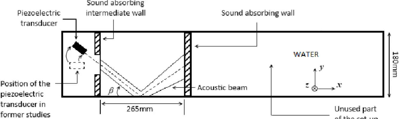
Experiments are performed in a rectangular cavity filled with water. A top view of the setup is presented in figure 1; this is actually a modification of the formerly presented ASTRID setup [7-9]. A 2 MHz circular plane transducer from Imasonic, with a diameter of 29 mm, is used to generate the acoustic beam. The investigation domain is delimited by two sound absorbing plates made of Apflex F28 tiles from Precision Acoustics™. The first plate (from left to right on the figure) is positioned close to the transducer. It is drilled with a 63 mm hole and covered with a thermo retractable plastic film to let the sound enter in the investigation area but, at the same time, provide a rigid wall condition for the generated steady flow. The second plate is the end-wall of the investigated area. In our former studies [7-9], the distance between the centers of the transducer surface and the plastic film was 10 mm and the second plate was set at 275 mm from the transducer surface center. In the present study, the positions of the film and plates are kept identical, but the transducer is displaced. A glass lid is moreover installed on top of the water in order to avoid the dissymmetry in the boundary conditions due to a free surface. The dimensions of the investigation volume delimited by the two sound absorbing plates and the side, top and bottom walls of the glass tank are thus 265 x 180 x 160 mm3 (length x width x depth).

As depicted in figure 1, the transducer is tilted from its original position along the tank axis so that it is now oriented towards a side wall and creates a beam in the middle horizontal xy plane (namely at 80

3

mm from the bottom and top walls). This acoustic beam impinges at the middle of the side wall with an angle  = 34°; it is then reflected towards the end-wall where it is absorbed (Fig. 1).

Figure 1: Experimental setup (top view). The origin of the Cartesian frame is set at the middle of the inner surface of the sound absorbing intermediate wall: x-axis is parallel to the lateral walls, y and z axis are respectively horizontal and vertical. The depth is 160 mm and a glass lid avoids the presence of a free surface.

A PIV (Particle Image Velocimetry) system is used to measure the velocity field in the horizontal middle xy plane for three electrical powers: P = 2, 4 and 8 W. It includes a continuous laser which emits light at a wavelength of 532 nm. Image acquisition is performed with a camera from

Stemmer Imaging with a resolution of 2048 x 2048 pixels and with a frequency of 5 Hz. In our measurements, 7500 images are acquired as soon as the transducer is switched on, so that acquisition lasts about 25 min. The de-ionized water that is used is seeded with 5 μm Polyamid Seeding Particles of density 1030 kg m-3 from Dantec. The temperature of water was measured to be 23 °C.

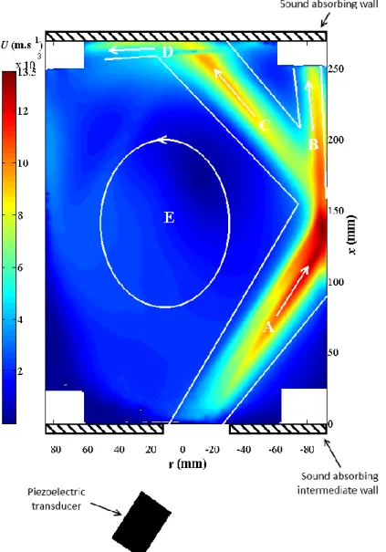
A typical experimental velocity field in the middle horizontal xy plane is presented in figure 2. Note that the white rectangles in the corners of the domain are due to obstacles in the field of view: these obstacles are the holders of the top lid, which are not in the fluid domain, but above. The velocity map shown in figure 2 is obtained with an electrical power of 8 W, but the same “y-shaped” flow structure is observed for the two other investigated electrical powers. This flow structure can be described as composed with 5 regions denoted A, B, C, D and E, which are delimited with white lines on the figure. While impinging the wall, the incident acoustic streaming jet (region A) splits into two jets: a wall jet moved by inertia (region B) and another acoustic streaming jet driven by the reflected acoustic beam (region C). This second acoustic streaming jet itself impinges the end-wall, where a second wall jet occurs (region D). Note that, as the acoustic beam is not reflected at this sound absorbing wall, this wall jet is the only jet generated in this area. These jets all together drive a large recirculation at the scale of the cavity in this middle plane (region E).

Submitted to Ultrasonics (2015)

4

Figure 2: Velocity magnitude obtained by PIV in the xy horizontal plane for an electrical power of P = 8 W. The piezoelectric transducer and the two absorbing walls are also represented as in figure 1. Four fastening systems, used to maintain the top wall, mask little zones at each corner, which appear as white squares. The observed “y-shaped” flow pattern is underscored by white lines. We distinguish 5 elements in the structure of this flow: A (incident acoustic streaming jet), B (first wall jet), C (reflected acoustic streaming jet), D (a second wall jet at the end-wall) and E (large recirculation at the scale of the cavity).

3. Numerical model

To simulate the flow, we consider a rectangular cavity with dimensions 265 × 180 × 160 mm3 (length × width × depth) filled with water. All the boundaries are considered as rigid walls with a no-slip condition. The computations are performed with the commercial software StarCCM+, which is used to solve the laminar, 3D, incompressible Navier-Stokes equations with an additional acoustic force term:

𝜌

𝑑𝑢⃗⃗

𝑑𝑡

= −grad

⃗⃗⃗⃗⃗⃗⃗⃗⃗⃗𝑝 + 𝑓⃗

+ 𝜇∆𝑢,

⃗⃗⃗⃗

(2)

where 𝑢⃗⃗ is the flow velocity (m s-1

), p is the hydrodynamic pressure (Pa),  is the fluid density ( = 1000 kg m-3),  is the dynamic viscosity ( = 10-3 Pa s) and 𝑓⃗𝑎𝑐 is the volumetric acoustic force (N m-3)

5

given by equation (1), with the sound attenuation  = 0.1 m-1, the celerity c = 1480 m/s and Iac

computed as described hereunder.

For a single transducer, the calculation of the acoustic intensity field is based on the Huygens-Fresnel assumption. The plane circular acoustic source is discretized with 200 x 200 elements. Each element with a surface S = α ( and α are the polar coordinates on the acoustic source surface) is considered as a secondary source emitting a spherical wave. The resulting acoustic intensity field is calculated at any location (x, y, z) in the fluid domain by superimposing each secondary source contribution (Rayleigh's integral). It is then expressed as:

𝐼

=

|Σ|

,

(3)

where Iac max is the maximal acoustic intensity, which is reached, for example, at the Fresnel length, 

is the wavelength and  is expressed as:

Σ = ∑ ∑

𝑒

√𝑥

_{+ 𝑦}

_{+ 𝑧}

_{+ 𝜎}

− 2𝜎

𝑦

cos(𝛼

) − 2𝜎

𝑧

sin(𝛼

)

σ

ΔσΔα,

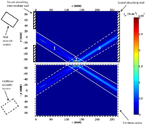
where (x’, y’, z’) are the coordinates of the points (x, y, z) of the fluid domain expressed in a frame of reference associated with the transducer: origin at the center of the transducer, x’ along the horizontal beam axis, y’ horizontal and transverse to the beam axis, z’ vertical. The beam reflection at the wall is accounted for by calculating the acoustic field generated by a fictitious source symmetrically disposed with respect to the side wall where the reflection occurs and superimposing it to the acoustic field generated by the real acoustic source, as depicted in figure 3. As previously mentioned, the angle is chosen to be 34°; for this angle, the reflection coefficient for the water-glass couple is equal to 1, as can be computed from the Snell-Descartes laws, so that the incident acoustic wave is completely reflected. The intensity delivered by the fictitious source is thus considered to be the same as that delivered by the real source. As a first approximation, the total acoustic intensity is then estimated by:

𝐼

=

4𝜆2

|Σ

+ Σ

|

,

(4)

despite the fact that the plane wave assumption might not hold in some regions of the resulting beam. The quantities real and fictitious are calculated, using equation (3), in the framework of the real and

fictitious source, respectively. Note that, in the case where a part of the incident acoustic wave is transmitted through the wall (i.e. the reflection is partial), the acoustic reflection coefficient is added as a multiplicative factor of fictitious in equation (4).

Figure 3 shows a typical acoustic intensity field obtained with this method; the upper part of the figure shows the real acoustic field while the lower part is the fictitious domain used for the calculation of the reflected beam. We describe the acoustic field as composed with three parts: the incident beam, here delimited by white solid lines (region 1), the reflected beam, delimited by white dashed lines (region 3) and the area where interferences occur between these two beams (region 2). This region 2 is numerically defined as a prism with vertical axis and triangular cross-section, located along the lateral wall at mid-length of the cavity and covering the interference zone (see figure 4a).

As can be seen from the intensity field pattern in the incident beam, the reflection wall is situated in the end part of the near-field region. In regions 1 and 3, the contribution of the reflected and incident acoustic beam, respectively, can obviously be neglected, so that the propagation direction is clear and the plane wave assumption holds. In region 1, the acoustic force field is thus computed from equation (1), oriented according to the propagation direction of the acoustic waves emitted by the real source. Likewise, the acoustic force field in region 3 is computed from equation (1), oriented according to the propagation direction of the acoustic waves emitted by the fictitious source.

Submitted to Ultrasonics (2015)

6

Figure 3: Acoustic intensity field in the xy horizontal plane with a reflection on the lateral wall for fac max = 4.05 N m -3

; the top part of the figure corresponds to the real domain; the bottom part is the fictitious domain; as a 100% reflection is considered, this configuration is fully symmetric with respect to the water-glass interface. The (real) transducer and the two absorbing walls are also represented for the real domain, as in figure 1.

The difficulty is to model the acoustic force field in region 2. A costly possibility would be to compute the acoustic velocity field, for instance from the compressible Euler equations, and to deduce the acoustic streaming force from a Reynolds-stress like computation or to use the inverse method developed by Myers et al. [33] where the acoustic force is computed from PIV velocity measurements. To overcome this time-consuming procedure, our strategy is, first, to evaluate the amplitude of the acoustic force with equation (1) where Iac is computed with equation (5), then, to implement several

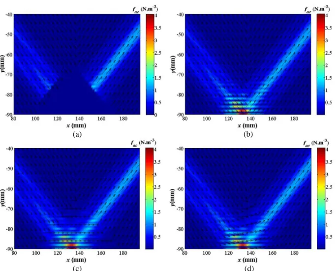
crude models for the direction of the acoustic force vector in region 2 and, finally, to compare the obtained velocity fields to the experimental data. As most of the momentum driving the flow is injected by the acoustic beams in regions 1 and 3, we can indeed expect this local modeling to have only little influence on the observed flow pattern, so that even a crude modeling can yield convenient results when compared to experimental data. Four models are considered and illustrated in figure 4, which is a zoom on region 2. The assumptions made for region 2 with these different models are:

- model a: zero force is applied,

- model b: the force field is computed from the incident beam on the left hand side of the impingement and from the reflected beam on its right hand side,

- model c: the force is assumed parallel to the wall, - model d: the force field lines are assumed circular.

7

(a) (b)

(c) (d)

Figure 4: Acoustic force field in the horizontal xy middle plane with (a) zero force, (b) incident and reflective force at each side of the impingement, (c) straight force parallel to the lateral wall and (d) circular force in the crossing zone. Colors provide information on the level of fac and normalized vectors are used to give the direction of fac.

The fluid domain is meshed with cubic cells; a mesh convergence study led us to choose 1 mm cells so that the total number of cells is 3 million. The acoustic force is computed with the Matlab software at each cell center from equation (1) through two steps: calculation of Iac and computation of fac. The

acoustic force level is characterized by the maximum value of the force, fac max, reached, for example,

on the beam axis at the Fresnel length. To compute the flow, we used the steady segregated solver implemented in StarCCM+™ for the two lower values of the acoustic force, but, for convergence reasons, the 2nd order unsteady segregated solver was preferred for the highest intensity of the acoustic force, with a time step of 1 second.

Submitted to Ultrasonics (2015)

8

(a) (b)

(c) (d)

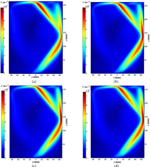
Figure 5: Numerically computed velocity magnitude in the horizontal xy middle plane for fac max = 1.75 N m-3 with (a)

model a, (b) model b, (c) model c and (d) model d, as explained in figure 4.

Typical velocity intensity fields obtained using the different force models are plotted in figure 5 for fac max = 1.75 N m

-3

. As can be seen on these colormaps, the observed flow pattern hardly differs from one model to another. The maximum velocity is found to be of 7 mm s-1 for the crudest model, model a, and 7.7, 7.9 and 7.9 mm s-1 for models b, c, and d, respectively. The discrepancy between these 3 last models is thus less than 3%, which is smaller than the experimental uncertainty on the velocity measurements. We thus consider that the result is only slightly dependent on the force model and decide to use model c in the rest of the study.

9

4. Results and discussions

(a) (b)

Submitted to Ultrasonics (2015)

10

(e) (f)

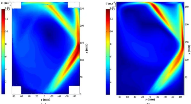
Figure 6: Velocity intensity fields in the horizontal xy middle plane for: (a) and (b) fac max = 1.75 N m-3, (c) and (d) fac max =

2.70 N m-3, (e) and (f) fac max = 4.05 N m -3

. On the left: (a), (c) and (e) experimental measurements using the PIV technique. On the right: (b), (d) and (f) numerical calculations with StarCCM+™ software. Note that four fastening systems, used to maintain the top wall, mask little zones at each corner, which appear as white squares in the experimental fields.

A comparison of experimentally measured and numerically computed velocity magnitudes in the xy middle plane, which contains the incident and the reflected beam axes, is shown in figure 6. As can be seen, the flow pattern is well reproduced by the numerical simulations. In particular the ‘y shape’ of the flow structure is observed and the relative flow intensities in the different branches of this structure correspond to those observed in the experiments. The complexity of the velocity profiles in the incident beam is also observed both numerically and experimentally: indeed, carefully looking at the region given by -80 mm < y < -50 mm and x ~100 mm, we can see that the jet is not a usual straight axi-symmetric jet.

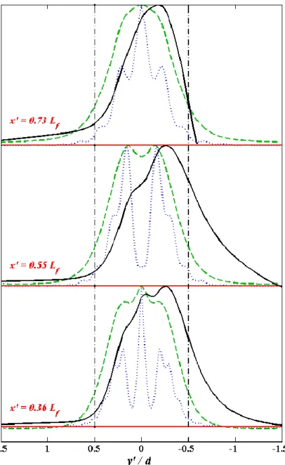
Such a complexity in transverse velocity profiles has formerly been observed for non-reflected centered acoustic streaming jets [6,9]. It was clearly correlated to diffraction patterns occurring in the acoustic near-field region: the acoustic intensity field features a number of local maxima inducing local accelerations, which distort the usual smooth shape of the velocity profiles. In the present case, an additional complexity is due to the bending of the jet towards the aquarium wall. Figure 7 gives a comparison of three normalized velocity transverse profiles in the incident beam (black solid lines), to their equivalent in the case of a centered acoustic streaming jet [9] (green dashed lines). Though the experimental configurations are not exactly the same, these profiles are plotted at the same distance x’ from the source along the acoustic beam: x’=0.36 Lf, 0.55 Lf and 0.7 Lf (Lf being the Fresnel length).

The sources used in both cases being the same, the normalized acoustic force profiles are identical before the interaction with the wall; they are plotted as blue dotted lines. Looking at the transverse location of the maximum velocity, we see a clear deviation of the jet with regard to the reference centered jet, which can reach up to a few millimeters. Note also that the transverse size of the jet in the incident beam is still comparable with the acoustic field diameter.

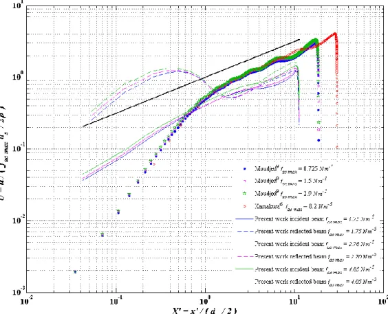
An interesting feature of the jets formerly observed by Moudjed et al. [9] was that a proper scaling allowed to plot on the same figure velocity profiles obtained with different experimental setups (see their figure 5). The appropriate scaling relies on the balance between the acoustic force and the inertia due to the flow acceleration along the jet; this yields the following scaling law for the variation of the velocity along the beam axis: U = X’1/2, where U = u/(f ds/2)

1/2

is the normalized velocity in the direction of the beam axis and X’ stands for the distance from the wall along the beam axis, scaled by the acoustic source radius, ds/2. The velocity profiles obtained numerically by Moudjed et al. [9] for a

11

centered beam aligned with the x axis of the cavity and for three investigated force values are reproduced in figure 8 as colored symbols, as well as the profile obtained in a similar configuration by Kamakura et al. [6]. The profiles along the incident beam are also plotted as solid lines, while the profiles along the reflected beam are plotted as dashed lines. Let us recall that the full black line is the scaling law U = X’1/2. The over-velocities observed in the reflected jet for X’<1 correspond to the region affected by the impingement of the incident jet. As can be expected, the size of this region scales with the acoustic source diameter. Note also that the initial variation of the velocity (for X’<1) in the tilted incident beam is different from what was obtained for a centered beam. In any case, for

X’>1, the expected X’1/2

scaling is quite nicely observed along the two jets. The observed velocity levels are, however, smaller than in both former studies with centered jets, which can partly be attributed to the bending of the jet in the present study: indeed this plot, along the acoustic beam axis, does not correspond to the maximum velocity in the jets.

Figure 7: Horizontal normalized profiles taken in the direction y’ transverse to the beam axis for: the experimental acoustic intensity (blue dotted lines), the numerical velocity in a centered, non-reflected, near-field acoustic streaming jet (from figure 5 of [9]) (black solid lines) and the numerical velocity in the incident beam in the present investigation for fac max = 2.70 N m

-3

(green dashed lines). These profiles are taken at the same distance x’ from the transducer along the acoustic beam axis, and plotted for three values of x’.

Submitted to Ultrasonics (2015)

12

Figure 8: Dimensionless plot of the longitudinal velocity profiles along the jets (incident and reflected) in the present study (full and dashed lines) in comparison to former studies with non-reflected centered acoustic streaming jets [6,9]. The full black line corresponds to the U = X’1/2

scaling law issued from the balance between the acoustic force and the inertia due to the flow acceleration along the jets.

Note that our 3D computations give access to a number of data that could not easily be accessed in the experiment, such as, for instance, the 3D shape of the jet illustrated in figure 9. This figure represents the jet envelope defined as the region in which the velocity magnitude exceeds a certain threshold value, here chosen as 4 mm/s. This plot particularly emphasizes the spreading of the jets around their impingement points. Friction at the wall and heat and mass transfer properties for this type of flow could also be computed, in link with peculiar applications, though this is outside the scope of the present paper. An interesting feature of such a flow pattern is that the main wall jet (region B) nearly reaches the corner of the tank, which could indeed be used to avoid heat or mass accumulation in this peculiar zone of the fluid domain.

13

Figure 9: 3D plot of the velocity magnitude isovalue at 0.004 m s-1. The left and the right hand sides of the figure give two different views of the impingement of the acoustic streaming jet on the lateral walls (view from the involved lateral walls and view from the inside of the cavity, respectively). Four of the five parts of the flow described in figure 1 are indicated here: incident jet A, first wall jet B (along the lateral wall), reflected jet C and second wall jet D (along the sound absorbing end-wall).

5. Conclusion

This paper presents the first experimental and numerical observation of Eckart acoustic streaming jets reflecting on a wall. The reflection of the acoustic beam driving the flow yields a peculiar ‘y-shape’ flow pattern, observed experimentally and well reproduced in the numerical simulations. The observed ‘y-shape’ flow pattern is due to the fact that the incident beam drives a jet that impinges on the lateral wall and creates a wall jet; at the same time, the acoustic beam is reflected on this lateral wall, which drives a second acoustic streaming jet forming an angle with the incident beam. The spreading of the jets around their impingement points and the creeping of the wall jets along the walls would allow the interaction of the flow with a large wall surface, which can even extend to the corners of the tank; this could be an interesting feature for applications requiring efficient heat and mass transfer at the wall. Confinement effects result in a significant bending of the incident jet; consequently the maximum velocity in a jet cross section can be a few millimeters far from the acoustic beam axis. Transverse profiles of the jet velocity exhibit complex shapes explained partly from this bending of the jet and partly from the complexity of the acoustic force field due to diffraction patterns, in particular in the acoustic near-field. The jet velocity profiles along the incident and reflected beam axis, however, feature the expected scaling from the balance between the acoustic force and inertia linked to the flow acceleration along the beam. This makes it possible to plot on the same figure velocity data obtained in very different experimental conditions (with and without reflections, different frequencies and source diameters, different acoustic intensities, etc.) and get a coherent picture.

A rough acoustic force model is shown to be sufficient to get a proper first order description of this rather complex flow. In particular this model relies on a standard linear acoustics approach, including diffraction effects, but the complex phenomena occurring in the interference zone of the incident and reflected beams are drastically simplified. A finer approach would, at least, include space and time resolved 3D computations of the unsteady compressible Euler equations in this zone and the determination of the force term through the Reynolds stress tensor based on acoustic velocities; this would, indeed, be a very costly and difficult task, obviously out of reach of our engineering approach.

Submitted to Ultrasonics (2015)

14

6. Aknowledgements

Funding for this project was provided by a grant, including a doctoral fellowship for Brahim Moudjed, from ARC Energies Région Rhône-Alpes.

The authors greatly acknowledge Marion Cormier and Ancelin Borel, who worked on this project as undergraduate students at the INSA de Lyon mechanical engineering department.

7. References

[1] W. L. Nyborg, “Acoustic Streaming,” in NonLinear acoustics, Academic Press., San Diego, 1998.

[2] S. J. Lighthill, “Acoustic streaming,” J. Sound. Vibr., vol. 61, p. 391, 1978.

[3] H. Mitome, “The mechanism of generation of acoustic streaming,” Electron. Commun. Jpn. Pt.

III: Fundam. Electron. Sci., vol. 81, p. 1, 1998.

[4] A. Nowicki, T. Kowalewski, W. Secomski, and J. Wojcik, “Estimation of acoustical streaming: Theoretical model, Doppler measurements and optical visualisation,” Europ. J. Ultrasound, vol. 7, p. 73, 1998.

[5] V. Frenkel, R. Gurka, A. Liberzon, U. Shavit, and E. Kimmel, “Preliminary investigations of ultrasound induced acoustic streaming using particle image velocimetry,” Ultrasonics, vol. 39, p. 153, 2001.

[6] T. Kamakura, T. Sudo, K. Matsuda, and Y. Kumamoto, “Time evolution of acoustic streaming from a planar ultrasound source,” J. Acoust. Soc. Am., vol. 100, p. 132, 1996.

[7] B. Moudjed, V. Botton, D. Henry, S. Millet, J.-P. Garandet, and H. Ben Hadid, “Oscillating acoustic streaming jet,” Appl. Phys. Lett., vol. 105, 184102, 2014.

[8] B. Moudjed, V. Botton, D. Henry, H. Ben Hadid, and J.-P. Garandet, “Scaling and dimensional analysis of acoustic streaming jets,” Phys. Fluids, vol. 26, 093602, 2014.

[9] B. Moudjed, V. Botton, D. Henry, S. Millet, J.-P. Garandet, and H. Ben Hadid, “Near field acoustic streaming jet,” Phys. Rev. E, vol. 91, 033011, 2015.

[10] H. C. Starritt, C. L. Hoad, F. A. Duck, D. K. Nassiri, I. R. Summers, and W. Vennart,

“Measurement of acoustic streaming using magnetic resonance,” Ultrasound Med. Biol., vol. 26, p. 321, 2000.

[11] M. A. Solovchuk, T. W. H. Sheu, M. Thiriet, and W.-L. Lin, “On a computational study for investigating acoustic streaming and heating during focused ultrasound ablation of liver tumor,”

Appl. Therm. Eng., vol. 56, p. 62, 2013.

[12] H. C. Starritt, F. A. Duck, and V. F. Humphrey, “An experimental investigation of streaming in pulsed diagnostic ultrasound beams,” Ultrasound Med. Biol., vol. 15, p. 363, 1989.

[13] H. C. Starritt, C. L. Hoad, F. A. Duck, D. K. Nassiri, I. R. Summers, and W. Vennart,

“Measurement of acoustic streaming using magnetic resonance,” Ultrasound Med. Biol., vol. 26, p. 321, 2000.

[14] G. Zauhar, H. C. Starritt, and F. A. Duck, “Studies of acoustic streaming in biological fluids with an ultrasound Doppler technique,” Br. J. Radiol., vol. 71, p. 297, 1998.

[15] G. Zauhar, F. A. Duck, and H. C. Starritt, “Comparison of the acoustic streaming in amniotic fluid and water in medical ultrasonic beams,” Ultraschall Med., vol. 27, p. 152, 2006.

[16] M. C. Schenker, M. J. B. M. Pourquié, D. G. Eskin, and B. J. Boersma, “PIV quantification of the flow induced by an ultrasonic horn and numerical modeling of the flow and related processing times,” Ultrason. Sonochem., vol. 20, p. 502, 2013.

[17] M. C. Charrier-Mojtabi, A. Fontaine, and A. Mojtabi, “Influence of acoustic streaming on thermo-diffusion in a binary mixture under microgravity,” Int. J. Heat Mass Transf., vol. 55, p. 5992, 2012.

[18] J. Klima, “Application of ultrasound in electrochemistry. An overview of mechanisms and design of experimental arrangement,” Ultrasonics, vol. 51, p. 202, 2011.

15

[19] A. Mandroyan, M. L. Doche, J. Y. Hihn, R. Viennet, Y. Bailly, and L. Simonin, “Modification of the ultrasound induced activity by the presence of an electrode in a sono-reactor working at two low frequencies (20 and 40 kHz). Part II: Mapping flow velocities by particle image velocimetry (PIV),” Ultrason. Sonochem., vol. 16, p. 97, 2009.

[20] C. M. Poindexter, P. J. Rusello, and E. A. Variano, “Acoustic Doppler velocimeter-induced acoustic streaming and its implications for measurement,” Exp. Fluids, vol. 50, p. 1429, 2011. [21] D. Gao, Z. Li, Q. Han, and Q. Zhai, “Effect of ultrasonic power on microstructure and

mechanical properties of AZ91 alloy,” Mater. Sci. Eng. A, vol. 502, p. 2, 2009.

[22] X. Jian, H. Xu, T. T. Meek, and Q. Han, “Effect of power ultrasound on solidification of aluminum A356 alloy,” Mater. Lett., vol. 59, p. 190, 2005.

[23] X. Jian, T. T. Meek, and Q. Han, “Refinement of eutectic silicon phase of aluminum A356 alloy using high-intensity ultrasonic vibration,” Scrip. Mater., vol. 54, p. 893, 2006.

[24] G. N. Kozhemyakin, L. V. Zolkina, and M. A. Rom, “Influence of ultrasound on the growth striations and electrophysical properties of GaxIn(1-x)Sb single crystals,” Solid State Elect., vol. 51, p. 820, 2007.

[25] G. N. Kozhemyakin, “Imaging of convection in a Czochralski crucible under ultrasound waves,”

J. Cryst. Growth, vol. 257, p. 237, 2003.

[26] G. N. Kozhemyakin, “Influence of ultrasonic vibrations on the growth of InSb crystals,” J. Cryst.

Growth, vol. 149, p. 266, 1995.

[27] L. V. Zolkina and G. N. Kozhemyakin, “Influence of ultrasound on the growth striations in GaxIn(1-x)Sb single crystals,” Funct. Mater., vol. 12, p. 714, 2005.

[28] X. Liu, Y. Osawa, S. Takamori, and T. Mukai, “Microstructure and mechanical properties of AZ91 alloy produced with ultrasonic vibration,” Mat. Sci. Eng. A, vol. 487, p. 120, 2008. [29] L. Yao, H. Hao, S.-H. Ji, C. Fang, and X. Zhang, “Effects of ultrasonic vibration on

solidification structure and properties of Mg-8Li-3Al alloy,” Trans. Nonfer. Met. Soc. Chin., vol. 21, p. 1241, 2011.

[30] Z. Zhang, Q. Le, and J. Cui, “Microstructures and mechanical properties of AZ80 alloy treated by pulsed ultrasonic vibration,” Trans. Nonfer. Met. Soc. Chin., vol. 18, p. s113, 2008.

[31] J. P. Garandet, N. Kaupp, D. Pelletier, and Y. Delannoy, “Solute segregation in a lid driven cavity: Effect of the flow on the boundary layer thickness and solute segregation,” J. Cryst.

Growth, vol. 340, p. 149, 2012.

[32] J. P. Garandet, N. Kaupp, and D. Pelletier, “The effect of lid driven convective transport on lateral solute segregation in the vicinity of a crucible wall,” J. Cryst. Growth, vol. 361, p. 195, 2012.

[33] M. R. Myers, P. Hariharan, and R. K. Banerjee, “Direct methods for characterizing

high-intensity focused ultrasound transducers using acoustic streaming,” J. Acoust. Soc. Am., vol. 124, p. 1790, 2008.