HAL Id: tel-02274422
https://pastel.archives-ouvertes.fr/tel-02274422
Submitted on 29 Aug 2019HAL is a multi-disciplinary open access archive for the deposit and dissemination of sci-entific research documents, whether they are pub-lished or not. The documents may come from teaching and research institutions in France or abroad, or from public or private research centers.
L’archive ouverte pluridisciplinaire HAL, est destinée au dépôt et à la diffusion de documents scientifiques de niveau recherche, publiés ou non, émanant des établissements d’enseignement et de recherche français ou étrangers, des laboratoires publics ou privés.
vehicles
Francisco Navas Matos
To cite this version:
Francisco Navas Matos. Stability analysis for controller switching in autonomous vehicles. Robotics [cs.RO]. Université Paris sciences et lettres, 2018. English. �NNT : 2018PSLEM050�. �tel-02274422�
Préparée à MINES ParisTech
Analyse de stabilité pour la reconfiguration de
contrôleurs dans de véhicules autonomes
Soutenue par
Francisco NAVAS
Le 28 Novembre 2018
Ecole doctorale n° 432
Sciences des Métiers de
l’Ingénieur (SMI)
Spécialité
Mathématiques, Informatique
temps-réel, robotique
Composition du jury :
Michel, BASSETUniv. d’Haute Alsace Président Mariana, NETTO
IFFSTAR Rapporteur
Youcef, MEZOUAR
Univ. Clermont Auvergne Rapporteur Lydie, NOUVELIERE
Univ, d’Evry Examinateur
Jorge, VILLAGRÁ
CSIC (Espagne) Examinateur
Fawzi, NASHASHIBI
INRIA Directeur de thèse
Vicente, MILANÉS
Acknowledgments
I would like to express my sincere gratitude to my supervisors Vicente Milanés and Fawzi Nashashibi for the continuous support of my Ph.D. thesis and research, for their patience, motivation, enthu-siasm, and immense knowledge. Their guidance helped me in all the time of research and writing of this thesis. I could not have imagined having better supervisors for my Ph.D. thesis.
I thank my fellow labmates in the Robotics and Intelligent Transportation Systems team at INRIA for the stimulating discussions, the help during experimental tests, and for all the fun we have had in the last three years.
Last but not the least, I must express my gratitude to my familiy and friends, Ales, Cris, David, Jared, Jorge, Julia, Pietro, Raoul and Raquel for their continued support and encouragement, and for their patience experiencing all the ups and downs of my research. I thank Pietro for his willingness to read countless pages of meaningless equations.
Contents
Acknowledgments i 1 Introduction 1 1.1 Motivation . . . 1 1.2 Objectives . . . 5 1.3 Manuscript organization . . . 5 1.4 Contributions . . . 6 1.5 Publications . . . 7 1.5.1 Journal articles . . . 7 1.5.2 Conference papers . . . 72 State of the art 11 2.1 Origins . . . 12
2.2 Australian National University . . . 13
2.2.1 Q offline control design . . . . 14
2.2.2 Direct adaptive Q-control . . . . 15
2.2.3 CL identification . . . 15
2.2.4 Iterated/Nested (Q, S) control design . . . . 15
2.2.5 Indirect adaptive (Q, S)-control . . . . 16
2.3 Technical University of Denmark . . . 17
2.4 Aalborg University . . . 18
2.5 Discussion . . . 20
3 Youla-Jabr-Bongiorno-Kucera parameterization 29 3.1 System description . . . 29
3.1.1 The nominal plant model . . . 29
3.1.2 The stabilizing controller . . . 31
3.2 Doubly coprime factorization . . . 33
3.3 All stabilizing controllers/Controller reconfiguration . . . 36
3.3.1 From a initial stabilizing controller to a final stabilizing controller . . . 37
3.3.2 From a initial stabilizing controller to several stabilizing controllers . . . 39
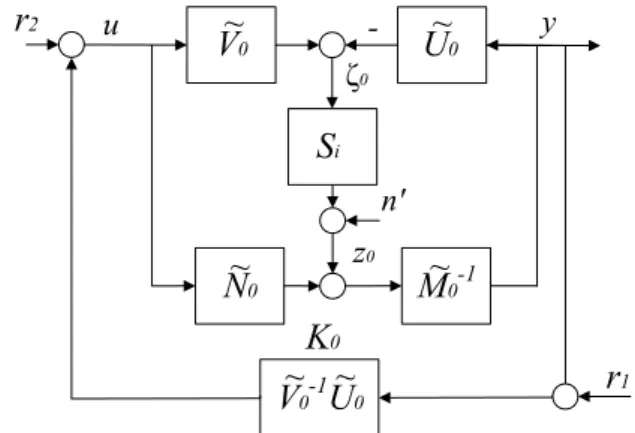
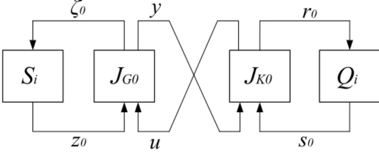
3.3.3 Controller structures . . . 42
3.4 Numerical examples . . . 46
3.4.1 Stable transition . . . 47
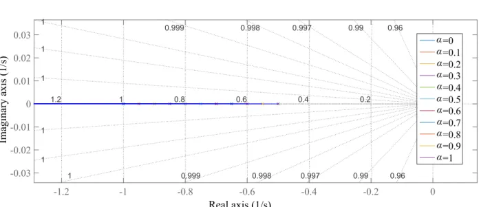
3.4.2 Root locus evaluation . . . 48
3.4.3 Transient behavior . . . 49
3.5 Conclusions . . . 53 iii
4 Dual Youla-Jabr-Bongiorno-Kucera parameterization 57
4.1 System variations . . . 57
4.2 Doubly coprime factorization . . . 58
4.3 All systems stabilized by a controller . . . 59
4.3.1 From a nominal model to a real model . . . 60
4.4 Adaptive control design . . . 61
4.4.1 Multi model adaptive control . . . 64
4.5 Dynamics identification . . . 67
4.5.1 Open-loop identification . . . 67
4.5.2 Closed-loop identification . . . 67
4.6 Conclusions . . . 72
5 Applications 75 5.1 Experimental platform and simulation models . . . 75
5.1.1 Cycab . . . 76
5.1.2 Nissan Infinity M56 . . . 78
5.2 YK controller reconfiguration . . . 78
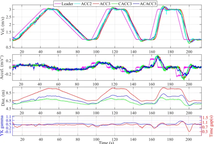
5.2.1 Cooperative adaptive cruise control . . . 79
5.2.2 Advanced cooperative adaptive cruise control . . . 82
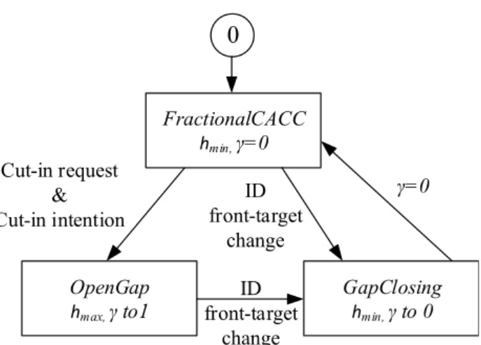
5.2.3 Cut-in/cut-out transitions in CACC systems . . . 93
5.3 Closed-loop identification . . . 104
5.3.1 Online closed-loop identification for longitudinal vehicle dynamics . . . 104
5.4 Adaptive control design . . . 111
5.4.1 Multi model adaptive control for cooperative adaptive cruise control appli-cations . . . 111
5.5 Conclusions . . . 123
6 Conclusions 127 6.1 Contributions to the state of the art . . . 129
6.1.1 Youla-Kucera parameterization . . . 129
6.1.2 CACC . . . 129
6.1.3 Autonomous driving . . . 130
6.2 Future research directions . . . 130
Chapter 1
Introduction
Autonomous vehicles are getting more and more attention because of their potential to both significantly reduce the number of road fatalities and improve drivers’ daily lives. Driverless cars research field has been very active in recent years, and significant advances have been achieved. However, there are still some significant gaps before having fully automated vehicles on public roads.
The research on the last years has been focused on the development of multi-sensor systems able to perceive the environment in which the vehicle is driving in, permitting to create a comprehensive map of the traffic situation. These multi-sensor perception systems are significantly increasing the complexity when it comes to autonomously control the vehicle. Different control systems are activated according to a multi-target decision making system. Each of these systems follows performance and stability criteria for its design, but they all have to work together, providing stability guarantees and being able to handle unexpected situations as unpredicted uncertainties or even fully outages from sensors. With these premises, the goal of this Ph.D. work is to further investigate intelligent advanced control systems to provide stable responses for autonomous vehicles under different circumstances.
This thesis has been developed within the Robotics and Intelligent Transportation Systems (RITS) team/project at the French National Institute for Research in Computer Science and Control (INRIA, from french: Institut National de Recherche en Informatique et en Automatique). In the following, the author explains motivation, objectives, manuscript organization and main contributions of the presented work.
1.1 Motivation
Autonomous driving aims to improve traffic flow, reduce accidents and fuel consumption, and make possible personal car travel for everyone regardless of their abilities or conditions. An autonomous vehicle is built by combining a set-of-sensors and actuators together with sophisticated algorithms. These algorithms perform different functions, taking the information coming from the sensors to make the vehicle react to different traffic situations through the actuators [Luettel et al., 2012]. A general architecture for autonomous driving is in Fig. 1.1. Details about each of the blocks that form this autonomous vehicle’s architecture are found below:
• Acquisition. It is the process on charge of getting information from the installed sensors in the vehicle. Global Position Systems (GPS), Inertial Measurement Unit (IMU) and odom-etry are used for vehicle location in a coordinate framework; Light Detection And Ranging
1.1. MOTIVATION 3 (LiDAR) sensors, radar, ultrasounds, and cameras are employed for having a 360º view of the environment.
• Communication. Vehicle to Vehicle (V2V) and Vehicle to Infrastructure (V2I) wireless com-munications are used to be able to communicate with other vehicles and road infrastructure. • Perception. This block uses the information coming from the acquisition stage, in order to understand and model the environment around the vehicle, being aware of its state in such environment. Obstacles detection in the surroundings (pedestrians, vehicles. . . ), ego-vehicle’s localization and detection of lane marks on the road, are some of the tasks linked to this block.
• Decision. It manages the data processed in the perception stage for a dynamic behavior of the vehicle. It is able to react and interact with unexpected situations that usually affect the predefined driving such as: pedestrians, road works, obstacles, Human-Machine-Interface (HMI) request, etc.
• Control. It is responsible for the reference path tracking and driving safety requirements provided by the decision stage. Control variables as steering angle and longitudinal velocity are obtained in order to correctly follow orders given by the decision stage.
• Actuation. The control output is sent to the different vehicle actuators: The steering wheel for the lateral control; and throttle, brake and gear shift for longitudinal control.
This PhD work is focused in the control block design. According to different scenarios (i.e. road layout, other traffic agents interaction), different control systems are required. Activation is commanded by the decision system based on the information provided by the perception block. Control systems can be divided in classical, optimal, robust, adaptive and Fault Tolerant Control (FTC):
• Classical control is based on the use of linear differential equations describing system dynam-ics. Control mission is to make the error between reference input and feedback sensor state zero.
• Optimal control, on the other hand, is an extension of classical control in which you answer the question: How do I design my controller to ensure that I optimize a performance index? It assumes a perfect model of the system.
• Robust control, on the contrary, assumes that the model is imperfect, seeking for stability and quality of the controller given external disturbances or uncertainty in the system model. • Adaptive control is required in scenarios where large changes occur. Controller parameters change with time and tracks the changes in the plant, with the goal of designing a system which, at all instants, performs in accordance with the design constraints.
• FTC aims to increase plant availability and reduce the risk of safety hazards. Its goal is to prevent that simple faults develop into serious failure.
Vehicle dynamic control can be divided in lateral and longitudinal controllers. The former allows to automatically steer according to a planned trajectory. The latter acts on the throttle and brake for folllowing a reference speed, playing a key role to ensure safety and comfort of passengers.
Specifically related to automated longitudinal control, Cruise control and platooning tasks are mainly developed. Cruise control permits to set a maximum speed at which someone desires to travel, acting over throttle and break pedals in order to maintain the speed of the vehicle even on up and down hills. By adding a forward radar, vehicle gains environmental information – intervehicle distance – to adapt its velocity according to the preceding’s one. This is called Adaptive Cruise Control (ACC). ACC reduces congestion in highways by making formation of vehicles. V2V communication is added to the existing ACC system, improving traffic flow through the formation of a tighter string of vehicles– so-called Cooperative Adaptive Cruise Control (CACC). While ACC/CACC are comfort systems to help the driver and reduce traffic congestion problem, they do not have a way to prevent a crash with a forward vehicle or pedestrian. These kind of systems are not full range, and another controller will be needed if preceding vehicle brakes suddenly or a pedestrian passes between two vehicles. Emergency brake control needs to be developed. Once both cruise and emergency brake control are designed, an optimization process could be carried out in order to make maneuvers optimal. This involves completing maneuvers, such as join, split or change lane in the minimum possible time, while maintaining as high a speed and as small a distance from the preceding vehicle as practicable and safe. Optimal acceleration/deceleration could be also treated in the sense of minimizing fuel consumption. All these solutions together significantly enhance road safety and improve highway utility. However, various uncertainties and disturbances present in the real world should be considered to have not only a optimal solution, but robust. Uncertainties or external disturbances are for example dynamics of different vehicles, variant delay communication between vehicles, wind gust or road slopes. When dynamics difference are large, and adaptive control with identification process would be needed. Finally, FTC is also employed in order to deal with communication link availability or in-wheel motor faults in electrical vehicles, among others. This shows the need to employ different control systems in order to have a complete solution dealing with different traffic situations, dynamics of ego and surrounding vehicles, sensor/actuators availability, pedestrians or even driver preferences.
Lateral control is in charge to turn the steering wheel for applying path corrections to reduce or remove errors between actual and intended paths. The intended path can change in order to avoid obstacles or pedestrians. It is clear that GPS, camara, odometry and LiDAR is needed in order to localize the vehicle with respect to the intended path. A classical solution should be able to navigate soft turns and straight lines at specific velocity. It is logical that the steering wheel of our car does not turn in the same way to take a curve, if this is done at 10km/h or 100km/h. Different controllers would be needed depending on the longitudinal velocity of the vehicle. At the same time, those controllers could be modified to cover a wide range of roads/situations, including sharp turns, roundabouts, lane change and so on. Adaptive control could offer a good adaptability to different road types and velocities. Robustness is also important in lateral control. Uncertainties are mainly in parameters as tire cornering stiffness, vehicle longitudinal velocity and yaw rate. A typical external disturbance is the road surface friction condition, which is uncertain and can change extremely quickly. It is not the same to drive in icy than in rough asphalt roads. To improve control, the road surface friction can be treated as a robust solution for a specific range, or even as an adaptive solution if an estimation of this parameter exists. Finally, FTC solutions would be also important to ensure accurate path tracking in the presence of faults. Faults could go from sensors fails to wheel lock. Consequently, lateral control needs different control solutions depending on the road form and situation, vehicle dynamics and sensor/actuators availability. Driver preferences could be also important in order to adapt driving style.
In short, both longitudinal and lateral control solutions have many different solutions depending on the nature of the problem, and a control/supervision structure would be necessary to deal with
1.2. OBJECTIVES 5 all the types of changes that may come. In this thesis, Youla-Kucera (YK) parameterization is analysed as a methodology that could improve the security of autonomous driving systems by providing a framework managing different sensor/actuator setups, dynamics and traffic situations with stability guarantees.
1.2 Objectives
The objective of this Ph.D. thesis is to further investigate the YK parameterization to provide stable responses for autonomous vehicles when dynamics or environmental changes occur. This thesis explores the use of the YK parameterization in dynamics systems such as vehicles, with special emphasis on stability when some dynamic change or the traffic situation demands controller reconfiguration.
In order to meet with the idea of general control framework handling those changes into the vehicle, different steps should be followed: First, controller reconfiguration due to different traffic situations is explored. Then, dynamics of ego or surrounding vehicles could be important in order to improve vehicle performance/stability. Thus, identification of unmodeled vehicle dynamics is analysed. Finally, both controller reconfiguration and dynamics identification should be used together following some performance/stability criteria.
Focus is in obtaining simulation and experimental results related to the use of the YK parame-terization in the longitudinal control of an autonomous vehicle. CACC applications are targetted, with the aim not only of using for the very first time YK parameterization in the Intelligent Transportation Systems (ITS) domain, but improving CACC state-of-the art by providing sta-ble controller reconfiguration results when non-availasta-ble communication link with the preceding vehicle, cut-in/out maneuvers or surrounding vehicles with different dynamics.
With the present results, the author aims to prove adaptability, stability and real implementa-tion of the YK parameterizaimplementa-tion as control framework for secure responses in autonomous driving.
1.3 Manuscript organization
The present Ph.D. work is organized in a total of six chapters. An overview of remaining chapters is given below:
Chapter 2. State of the art. This chapter presents a review of the YK parameterization related to classical, optimal, adaptive, robust and FTC. The origins of this mathematical framework are explained. Important groups worldwide are reviewed, focusing on the different types of control applications developed, allowing the understanding of open challenges and future research work.
Chapter 3. Youla-Jabr-Bongiorno-Kucera parameterization. YK parameterization provides all stabilizing controllers for a given plant, and this is used for performing stable con-troller reconfiguration. YK mathematical basis is provided with emphasis in stability proof. Dif-ferent control structures for stable switching are derived from this parameterization, dealing with problems such order complexity, plant disconnection or matrix inversability. Different numerical examples are given for the better understading of the stable controller reconfiguration and transient behavior depending on the chosen YK-based control structure.
Chapter 4. Dual Youla-Jabr-Bongiorno-Kucera parameterization. Dual YK parame-terization provides all plants stabilized by a given controller, and this is used to perform controller design in the presence of system variations or Closed-Loop (CL) identification. The basis of this parameterization is also explained. CL stabilization in the presence of system variations is
anal-ysed. The dual YK parameterization properties are used for obtaining a Multi Model Adaptive Control (MMAC) approach, and CL identification algorithms.
Chapter 5. Applications. This chapter explores the uses of YK and dual YK parameteriza-tion in autonomous driving; specifically, CACC applicaparameteriza-tions are considered in the presence of traffic or dynamics changes. YK-based stable controller reconfiguration is used to deal with the problem of non-available communication link with the preceding vehicle; and vehicles joining/leaving the string. Then, as vehicles in the string could be different, dual YK parameterization is employed to perform CL longitudinal dynamics identification. Finally, both YK and dual YK parameterization are used in a MMAC approach to deal with vehicles heterogeneity in CACC string of vehicles. Simulation and experimental results with different type of controllers and structures prove adapt-ability, stability and real implementation of the YK parameterization.
Chapter 6. Conclusions. Conclusions and most important remarks, with respect to the problems addressed in the present Ph.D. work, are given in this chapter. Also future research lines are presented and discussed.
1.4 Contributions
In the present dissertation, YK parameterization is used as control framework able to deal with controller reconfiguration, dynamics identification and adaptive control approaches. Contributions are detailed below:
1. YK parameterization provides all stabilizing controllers for a given plant. This is used in order to perform stable controller reconfiguration. Different YK-based control structures are ob-tained for dealing with problems such order complexity, plant disconnection or matrix inversability. Stability properties are preserved even if different structures are employed, but transient behavior between controllers changes depending on the employed YK-based structure. One of the structures presents the best transient behavior without oscillations, a lower order controller complexity and no need to disconnect the initial controller, which would be important if the system shutdown is very expensive, or the initial controller is part of a safety circuit. This structure is used together with CACC applications improving CACC state-of-the-art. A hybrid behavior between two CACC controllers with different time gaps is explored by means of the YK parameterization, in order to avoid ACC degradation when communication link with preceding vehicle is lost. The proposed system uses YK parameterization and communication with a vehicle ahead (different from the preceding one) providing stable responses and, more interestingly, reducing intervehicle distances in comparison with an ACC degradation. A similar idea of hybrid behavior between CACC con-troller with different time gap is developed for entering/exiting vehicles in the string. In that case, YK parameterization is able to ensure stability of these merging/splitting maneuvers.
2. Dual YK parameterization provides all the plants stabilized by a controller. This is employed for solving CL identification problems, or adaptive control solutions, which integrate identification and controller reconfiguration processes. YK-based CL identification uses classical OL identifica-tion algorithms, providing better results than if it is used alone. Results in a CACC-equipped vehicle prove how CL nature of the data affects a classical OL identification algorithm, and how dual YK parameterization helps to mitigate these effects. Finally, an adaptive control application is developed by using MMAC. Longitudinal dynamics of two vehicles in a CACC string are esti-mated within a model set, so the good CACC sytem can be chosen even if a heterogeneous string of vehicles is considered. Dynamics estimation results much faster than other estimation processes in the literature.
1.5. PUBLICATIONS 7 adaptability of the YK parameterization to any type of controller. Simulation and experimental results demonstrate real implementation of stable controller reconfiguration, CL identification and adaptive control solutions dealing with dynamics changes or different traffic situations. The author thinks that YK is a suitable control framework able to ensure responses in autonomous driving.
1.5 Publications
As results from the work in the development of the Ph.D. thesis, the author cites the following publications:
1.5.1 Journal articles
Title: Youla-Kucera based Advanced Adaptive Cruise Control. Authors: F. Navas, V. Milanés and F. Nashashibi.
Journal: IEEE Transactions on Vehicular Technology. Status: Second revision submitted October 2018.
Title: Multi Model Adaptive Control for CACC applications. Authors: F. Navas, V. Milanés, C. Flores and F. Nashashibi. Journal: Control Engineering Practice.
Status: Second revision submmited September 2018.
Title: Youla-Kucera based Fractional Controller for Stable Cut-in/Cut-out Transitions in Cooperative Adaptive Cruise Control Systems.
Authors: F. Navas, R. de Charette, C. Flores, V. Milanés and F. Nashashibi. Journal: IEEE Transactions on Intelligent Transportation Systems.
Status: Submitted September 2018.
Title: A Cooperative Car-Following/Emergency Braking System With Prediction-Based Pedestrian Avoidance Capabilities
Authors: C. Flores, P. Merdrignac, R. de Charette, F. Navas, V. Milanés and F. Nashashibi. Journal: IEEE Transactions on Intelligent Transportation Systems
Number: 99 Pages: 1-10 Year: 2018.
1.5.2 Conference papers
Title: Youla-Kucera based lateral controller for autonomous Vehicle.
Authors: I. Mahtout, F. Navas, D. González, V. Milanés and F. Nashashibi.
Proceedings: 21st IEEE International Conference on Intelligent Transportation Systems Place: Hawaii, USA Date: November 2018.
Title: Youla-Kucera control structures for switching.
Proceedings: 2nd IEEE Conference on Control Technology and Applications. Place: Copenhagen, Denmark Date: August 2018.
Title: Youla-Kucera based online closed-loop identification for longitudinal vehicle dynamics. Authors: F. Navas, V. Milanés and F. Nashashibi.
Proceedings: 21st IEEE International Conference on System Theory, Control and Computing. Place: Sinaia, Romania Date: October 2017.
Title: Using Plug&Play Control for stable ACC-CACC system transitions. Authors: F. Navas, V. Milanés and F. Nashashibi.
Proceedings: 2016 IEEE Intelligent Vehicles Symposium. Place: Gothenburg, Sweden Date: June 2016.
Chapitre. État de l’art
Below is a French summary of the following chapter "State of the art".
Au sein de l’automatisme, l’ingénierie du contrôle est considérée comme une technologie ma-ture et cela de différentes manières. Elle s’inclut quasiment dans chaque type d’application dans le monde de l’industrie. La littérature regorge d’algorithmes de contrôle de systèmes, aussi com-plexes que soient les situations. Cependant, en pratique, de nombreux problémes apparaissent au moment de l’implémentation et plus particuliérement quand le système inclut des changements dynamiques, structuraux ou environnementaux. Pour résumer, beaucoup d’outils existent pour concevoir des contrôleurs appliqués aux systèmes dont la structure est connue. Toutefois, ces derniers ne fournissent pas les mêmes performances quand la structure du système contrôlé change au fil du temps. Le probléme de concevoir un contrôleur capable de traiter ces changements n’est pas nouveau. On peut citer le "Fault Tolerant Control" (FTC) spécialisé dans le cas des composants tombant en panne. Cependant, le travail dans le domaine est généralement limité par un nombre de pannes spécifiques auxquelles s’ajoute le probléme de l’apparition de nouveaux composants. Un autre domaine qui considère le changement au sein des systèmes est le contrôle adaptatif qui permet de suivre des changements pouvant être définis par la variation des paramètres du système controlé. Les changements nécessaires à la reconfiguration du système doivent être identifiés d’une manière ou d’une autre. Lorsque ces changements sont modélisés par des variations paramétriques prédéfinis, les changements structuraux ou l’introduction d’une nouvelle dynamique ne le sont pas. On retrouve aussi le contrôle robuste qui considère, quant à lui, un système dont les caractéris-tiques changent avec incertitudes. Quand ces incertitudes sont limitées, ce contrôleur fixe, garantit un comportement acceptable. Cependant, ce dernier n’est pas concevable dans les scénarios où ces changements sont trop importants. Les structures hiérarchiques gérant les changements des structures, à un instant précis, ont aussi été largement étudiées dans les domaines du contrôle dé-centralisé, distribué, hiérarchique et réseau. Traiter ces changements structuraux, implique aussi des transitions d’un système à un autre. Le domaine de "bumpless transfer" étudie le comportement des contrôleurs pendant la transition entre différent systèmes. Pour conclure, il y a différentes solu-tions dépendantes de la nature du problème. De plus, une structure de contrôle et de supervision, doit être appliquée lorsque différents types de changements interviennent.
La paramétrisation de Youla-Jabr-Bongiorno-Kucera (YK) est un outil de contrôle qui est ap-paru simultanément dans [Kučera, 1975,Youla et al., 1976a,Youla et al., 1976b]. La paramétrisation YK fournit tous les contrôleurs stabilisant un système donné. Ces derniers sont paramétrisés par la fonction de transfert appelée paramètre YK Q et donc : K(Q). Il peut être utilisé pour réaliser la reconfiguration stable du contrôleur quand différents changements interviennent. Le contrôleur en question peut être classique, adaptatif, optimal ou robuste. Mélanger différents types de con-trôleur est permis dans cette reconfiguration. La théorie duale de la paramétrisation YK, fournit
tous les systèmes stabilisés par un contrôleur donné. L’ensemble de tous les systèmes stabilisés par un contrôleur dépend de la fonction de transfert appelée paramètre YK dual S, ce qui donne: G(S). Ce paramètre peut représenter la variation paramétrique, les incertitudes de modélisation, changement de point d’opération .... Ce dernier est employé pour les identifications dynamiques et/ou l’identification de nouveaux capteurs/actionneurs connectés au système. Finalement, les deux paramètres YK peuvent être utilisés ensemble et ainsi une structure de contrôle qui change, basé sur des identifications dynamiques, est obtenue. Comme les capteurs/actionneurs sont iden-tifiés, le contrôle hiérarchique et le FTC sont ainsi réalisable par la paramétrisation de YK. Le contrôleur est modifié en fonction des nouvelles dynamiques, avec différents critères de performance et de stabilité. Avec ces hypothèses, YK est capable de répondre à toutes les solutions proposées au dèbut de ce chapitre avec la même structure théorique, tout en garantissant la stabilité. Par conséquent, il peut servir d’outil général de contrôle pour les systèmes exposés aux changements dynamiques, structuraux ou environnementaux.
Ce chapitre donne un aperçu du domaine de recherche de la paramétrisation YK. Les origines de cette technique sont expliquées. Les travaux principaux à travers le monde sont étudiés, en se concentrant principalement sur les différents domaines d’application du contrôle basé sur cet outil mathématique. Les applications sont classées en fonction de l’utilisation de Q, de S ou bien des deux.
Chapter 2
State of the art
Control engineering is considered as a mature technology in many different ways, being able of dealing with almost any kind of application in the industrial context. The literature is rich in algorithms to design control systems, even highly complex control problems. But, in practice, several problems appear for its implementation, especially when the system is exposed to dynamics, instrumental or environmental changes. In short, a lot of tools exists to design feedback controllers for a system with a known structure, but they are not providing proper responses when the structure of the system to be controlled changes over time. The problem of designing a controller able to deal with these changes is not new: Fault Tolerant Control (FTC) specializes in the case of components that fail. The work in this area, however, is usually limited to a prespecified amount of faults, and the problem of handling new components is not addressed. Another field that considers changing systems, it is the adaptive control area, which allows tracking changes that can be defined as parameters in the controlled system. Changes for controller reconfiguration need to be identified somehow. Since those changes are already set as predefined parameters, structural changes or new dynamics introduction are not considered either. On the other hand, robust control considers a system that changes their characteristics over time through uncertainties. These changes are somewhat bounded, so a fixed controller can be designed, guaranteeing an acceptable behavior. However, robust control design is not possible in scenarios where changes in the system are large. Hierarchical structures to deal with running structural changes have been also widely studied in the areas of decentralized, distributed, hierarchical or networked controls. Handling these structural changes also involves dealing with the transients when changing from one system to the other. Considerations about transient behavior when doing controller reconfiguration can be found on the bumpless transfer control area. In short, there are many different solutions depending on the nature of the problem, and a control/supervision structure would be necessary to deal with all the types of changes that may come.
Youla-Jabr-Bongiorno-Kucera (YK) parameterization is a control framework that appeared simultaneously in [Kučera, 1975, Youla et al., 1976a, Youla et al., 1976b]. YK parameterization provides all stabilizing controllers for a given system. All stablizing controllers are parameterized based on the transfer function called YK parameter Q, so K(Q). It can be used to perform stable controller reconfiguration when some change occurs. The type of controller could be any– classical, adaptive, optimal or robust control. Mixing different types of controller is allowed in this controller reconfiguration. The dual theory, dual YK parameterization, provides all the plants stabilized for a given controller. The class of all the plant stabilized by a controller depends on the transfer function called dual YK parameter S, so G(S). This parameter could represent any plant variations, uncertainties, parameter variations, change of operation point, etc. This
is employed for dynamics identification and/or identification of new sensors/actuators connected to a system. Finally, both can be used together, so a control structure that changes based on identified dynamics is obtained; as sensors/actuators are identified, hierarchical and fault tolerant control structures are also supported by YK. Controller is changed depending on new dynamics with some performance/stability criteria. With these premises, YK is able to encompass all the solutions proposed at the beginning of this chapter within the same theoretical framework and with stability guarantees. Thus, it could serve as a general control framework to deal with systems exposed to dynamics, instrumental or environmental changes.
The present chapter gives an overview of the YK parameterization research field. The origins of this technique are explained. Important groups worldwide are reviewed, focusing on the different type of control applications by using this mathematical framework. Applications are divided depending on whether Q or S are used, or both.
2.1 Origins
G(s)
y
u
K(s)
r
-Figure 2.1: Negative feedback loop.
The origin of YK is in [Newton et al., 1957]. Given a Single-Input-Single-Output (SISO) stable plant, they found a way to parameterize all the controllers that stabilize it. Let’s assume a feedback loop as in Fig. 2.1. If a stable controller K(s) is connected to the plant G(s) in a negative feedback loop, the transfer function of the control input u from the reference signal r yields:
Q(s) = U (s) R(s) =
K(s)
1 + K(s)G(s) (2.1)
where if Q(s) and G(s) are known, the controller transfer function K(s) can be recovered as follows:
K(s) = Q(s)
1 − G(s)Q(s) (2.2)
From Eq. 2.2, it is clear that if K(s) is a stabilizing controller, Q(s) is stable and proper; thus any stable and proper transfer function Q(s) represents a stabilizing controller for G(s). The class of all stabilizing controllers for a plant is obtained. This could seem useless, but they observed that the nonlinear transfer function from reference r to output y in K(s) becomes linear in Q(s) (see Eqs. 2.3 and 2.4 respectively). Thus, the design of Q(s) to achieve a desired performance is linear, obtaining K(s) by back-substitution.
Y (s) R(s)(K(s)) = K(s)G(s) 1 + K(s)G(s) (2.3) Y (s) R(s)(Q(s)) = Q(s)G(s) (2.4)
2.2. AUSTRALIAN NATIONAL UNIVERSITY 13 This idea of reparameterizing a set plant-controller in order to obtain linearity reappeared in [Zames, 1981]; and is well known as internal model control in chemical control process [Morari and Zafiriou, 1989]. But, it was not able to be applied for Multi-Input-Multi-Output (MIMO) systems.
[Kučera, 1975] and [Youla et al., 1976a,Youla et al., 1976b] proposed simultaneusly discrete and continous solutions to deal with MIMO unstable plants– so-called Youla-Kucera parameterization. There are two key points in the solutions: First, an initial stabilizing controller is considered; and second, plants are described using stable polynomial fractional transformations. Its use permited to see the plant as the combination of two stable transfer functions– e.g. an unstable plant G(s) = 1/(s − 5) is represented by X(s)Y (s)−1 with X(s) = 1/(s + 1) and Y (s) = (s − 5)/(s + 1).
These factors were employed in order to obtain an equivalent to Q(s) in Eq. 2.1. This new Q(s), called YK parameter, characterizes the class of all stabilizing controllers depending on stable polynomial fractional factors for G(s) and an initial K(s). Linearity was preserved even if stable polynomial fractional factors were used.
This approach was updated with coprime factors in order to avoid algebraic difficulties as noticed by [Desoer et al., 1980] and [Vidyasagar, 1985] for SISO and MIMO systems. An efficent method for obtaining these factors is based on a state-space representation [Nett et al., 1984]. As those coprime factors are the basis for obtaining the class of all stabilizing controllers, this state-space representation is preserved in almost every future application.
The linearity of Q within the Closed-Loop (CL) function facilitates optimization over the class of all stabilizing controllers. Every single controller could be augmented with Q. This Q is seen as a stable filter that can be optimize offline or online in order to improve system’s performace. An adaptive Q technique could be no longer useful when systems variations or uncertainites are large. A controller solution for such situations is provided by the dual YK parameterization.
Coprime factors of an inital plant connected to a stabilizing controllers are used in order to obtain the class of all plants stabilized by a controller. The connection between the dual YK and YK parameterizations was first developed by [Tay et al., 1989a], giving robust stability results. This dual YK parameter was used to suppress CL identification difficulties in [Hansen et al., 1989, Schrama, 1991]. The identification of a plant in the presence of a feeedback loop could be complex due to the noise. Given an initial model and controller, by identifying the dual YK S instead of G(s), the CL problem is transformed into an Open-Loop (OL) like problem. This is called in the literature Hansen scheme. The resulting S is used to carefully redesign the filter Q such that a better performance is achieved without loosing the stability of the system.
Performance enhancement techniques working with an adaptive Q are seen particularly in the work of the Australian National University. It is also there that the dual YK parameterization and robust stability results were first developed. Later, the Technical University of Denmark analysed Q as a fixed filter, focusing in stable controller reconfiguration properties. Stable controller recon-figuration through Q is combined with a fault-detection system through the dual YK parameter S, obtaining a Fault-Tolerant-Control (FTC) solution. Finally, some results are in proceeding with structural changes through S at the University of Aalborg. A more detailed review of the YK de-sign methodologies at the Australian National University, in the Technical University of Denmark and at the Aalborg University is in the following three sections.
2.2 Australian National University
The department of System Engineering, Research School of Information Sciences and Engineering at the Australian National University was the pioneer in using YK parameterization, to get what
they called high performance control. The concept of high performance control is to use the tools of classical, optimal, robust and adaptive control in order to deal with complexity, uncertainty and variability of the real world. They aimed to find a mathematical framework able to join performance and robustness.
First steps in this direction were made by John Moore at 1970s, on a high order NASA flexible wing aircraft model with flutter mode uncertaintiess. Least square identification was used in order to have an adaptive loop based on linear quadratic optimal control able to achieve robustness to these uncertainties. However, the blending betweeen adaptive and robust control lacked a mathematical framework. A collaboration with Keith Glover at Cambridge University allowed them to discover the interpretation of the YK parameterization as a general solution to optimal control problem provided by [Doyle, 1983]. Doyle characterized the class of all stabilizing controller as an initial Linear-Quadratic-Gaussian (LQG) controller with a stable filter Q, what fits the adaptive filter that they put in their solution for the aircraft model. A graduate student, Teng Tiow Tay started working on how to use that theory, obtaining really encouraging results. Initial point of his thesis with Moore as supervisor [Tay et al., 1989b]. Different applications related to YK formed a new field of research. We refer to book [Tay et al., 1997] and article [Anderson, 1998] as principal referees for undestanding how to use YK parameterization towards high performance control. Different techniques and applications related to that are detailed below:
2.2.1 Q offline control design
An offline optimization of Q was carried out in order to achieve various performance objectives. The idea is to design a controller in the class of all stabilizing controllers instead of over the class of all possible controllers (which includes destabilizing controllers). Different control performance objectives can be set in order to optimize the YK filter Q. Performance requirements can be described in time or frequency domain. System norms in the frequency domain is directly related to optimal control. H∞ is concerned primarily with the peaks in the frequency response, while
H2 is related to the overall response of the system. The idea is simple, once a transfer function
between different signal of interest is determined, H∞control designs a stabilizing controller that
ensures that the peaks in the transfer function are knocked down; on the contrary, H2 or LQG
control designs a stabilizing controller that reduces the H2 of the transfer function as much as
possible. Penalization of the energy of the tracking error and control energy are examples of LQG control; while penalizing the maximum tracking error subject to control limits is an example of H∞ control.
The design of an LQG controller with loop transfer recovery was analysed. This LQG controller uses a state estimator with the aim of estimating the non-accesible states of the plant. Its aim is to minimize error tracking and control effort. The controller will be optimal if a good model of the plant has been considered, otherwise the performance could be poor. Loop transfer recovery refers to the idea of reconfiguring the initial LQG controller to achieve full or partial loop transfer recovery of the original feedback loop. This is usually done through a scalar parameter as a trade-off between performance and robustness. In [Moore and Tay, 1989], loop recovery was achieved by augmenting the original LQG controller with the additional YK filter Q. They showed how full or partial loop recovery may be obtained depending if minimum or non-minimum phase plants are considered. The technique was ilustrated for the case of minimum and non-minimum phase plants through simulation. Improvements over standard loop recovery techniques were obtained.
The CL transfer function including Q from a disturbance input to a tracking error with a H∞
norm is in chapter 4 of [Tay et al., 1997]. This equation is useful to keep the tracking error within a given tolerance. However, minimizing the tracking error could lead sometimes to large control
2.2. AUSTRALIAN NATIONAL UNIVERSITY 15 efforts, what would be unnaceptable. As weighting factors between tracking error and control effort in a H∞setup is not allowed [Dahleh and Pearson, 1986], a l1 equivalent was proposed in [Teo and
Tay, 1995]. This algorithm allows to choose the correct weighting factors in a l1 manner. A curve
with all the possible solutions is generated for a simulation example, analysing the limitations and choosing the best weighting factors. This strategy is used in a hard disk servo system to minimize the maximum position error signal [Teo and Tay, 1996], which is the deviation of the read/write head from the center of the track.
2.2.2 Direct adaptive Q-control
In the previous section, an offline optimization of the YK parameter Q has been explained. [Wang et al., 1991] presented the first results in online optimization of Q without an identification process. The method is valid when the uncertainty is limited but unknown, and the plant-model mistmatch is not important. The optimization process is based on root-mean-square signals measures. A state-space relationship between a nominal plant with disturbances and a observer-based feedback controller K(Q) is obtained. The order of Q should be fixed depending on the application. A steepest descent algorithm is used to obtain the parameter values of the predefined YK parameter Q, so the error is minimized from the disturbances on the system. Simulation results of the direct adaptive-Q controller were presented in [Tay and Moore, 1991] to ilustrate their performance enhancement capabilities when disturbances appear on the system. Part of these results were previouysly validated in a 55th order aircraft model with a controller design via LQG with Q augmentations for achieving resonance suppression in [Moore et al., 1989].
In chapter 6 of [Tay et al., 1997], this method was analyzed to discover its limitations. First, a perfect plant model with disturbances was considered, achieving again without problems an optimal control. Then, the model-plant mistmach case was analysed, seeing how the adaptive mechanism breaks down under severe model-plant mismatch. An identification algorithm would be needed when a large model-plant mistmach is present. Section below presents an extension of the first YK-based CL identification algorithm– Hansen scheme.
2.2.3 CL identification
CL identification provided by [Hansen et al., 1989] is extended when connected to a controller with the YK filter Q in chapter 5 of [Tay et al., 1997]. Robust stabilization results in [Tay et al., 1989a] connecting K(Q) and G(S) are used to obtained an unbiased identification of S when a YK parameter Q is applied. A time-invariance property of Q is considered in the result. The unbiased CL identification of S is done through the identification of ˆS = S(I − QS)−1, which includes Q.
In order to obtain the real value of S, Q needs to be known. This CL identification method is the basis of the iterated (Q, S) control design shown below.
On the other hand, the original Hansen scheme is also extended with a non-linear initial model G(s) connected to a stabilizing controller K(s) in [Linard and Anderson, 1996, Linard and Anderson, 1997]; and [De Bruyne et al., 1998] presented a modification able to tune the order of the resulting model given by the Hansen scheme.
2.2.4 Iterated/Nested (Q, S) control design
This section considers solutions with unmodeled dynamics in the nominal model of the plant. K(Q) is seen as a controller where Q is changed online, as well as G(S) is seen as a nominal plant with an augmentation related to unmodeled dynamics. The process is the following: First, a
nominal controller K(s) is designed for a nominal plant G(s). Plant-model mistmatch is identified through the dual YK parameter S, and then the augmented controller Q is designed to optimally control S to some performance criteria. The performance is usually the same that the one used for the initial controller. These ideas are based on the robust stabilization concept in [Tay et al., 1989a]. Iterative and nested solutions are present in chapter 5 of [Tay et al., 1997].
For iterative control (Q, S) design, an initial stabilizing controller is designed for the nominal plant G(s). Then, unmodeled dynamics represented by ˆS are identified by using the CL identifica-tion method proposed in [Tay et al., 1997]. It avoids bias problems in the identificaidentifica-tion process. ˆS is used in an iterative manner for finding the Q that improves the performance criteria. Iteration is needed as the value of ˆS won’t be reliable enough at the very beginning or due to new deficiencies in the model. In each iteration the order of the controller increases as ˆS includes the applied Q, followed by a control update step. The sucess of this method relies on the use low-order approx-imations of S. Controller reduction will be also crucial in practical implementation. Simulation results related to Iterated Pole-Placement, Linear-Quadratic (LQ) control design and H∞ control
are in [Tay et al., 1997].
For nested control (Q, S) design, succesives S are identified on the residual mistmatch between model and plant. An external signal needs to be injected in order to identify the new S. In each step the model of the system is updated. This new model is then taken into consideration for obtaining a new Q, until the performance criteria is fulfilled. This kind of structure is practical when a plant is described by m recursive fractional forms. It could be the case of a complex model composed by low order models, so the controller could be broken down into a sequence of low order controller designs for a sequence of low-order models. Thus, a S is identified for each fractional form of the model, and a Q affined in the nested control structure.
2.2.5 Indirect adaptive (Q, S)-control
Sometimes, the major limit is the little knowledge about the plant. In such cases, iterated and nested control designs have been proposed. But, these algorithms are limited to a time-invariance Q property. In order to deal with a time variance Q, an adaptive version of nested control was proposed in [Tay et al., 1989b]. In any adaptive algorithm a fixed structure of Q is created. Parameters in Q are the ones changing depending on the model-plant mistmach identified by S. Notice how the unbiased identification provided in previous sections is no longer available as Q varies with time. External excitation signals are needed in order to identify S, and this could compromise the control performance. Two methods were proposed to solve that:
The use of two different time scales in the adaptive algorithm, a faster one for the identification of S, and a much slower for the adaptation of Q. This idea was proposed in the PhD thesis [Wang, 1991].
In chapter 7 of [Tay et al., 1997] a different method is explored. They considered that the model-plant mistmatch is significant in a frequency range above the passband of the nominal control loop. In fact, if Q is present on the system, the identification of S is frustrated. In order to solve that, the idea was to augment Q with a filter in the frequency of the excitation signals needed for the identification of S. The filtered excitation algorithm provides a suitable method for including external signal in a particular frequency range to identify S, without compromising the control performance.
A 55th order aircraft model was used in the literature for obtaining results that validates indi-rect (Q, S)- control. Adaptive LQG and pole-placements solutions were presented in [Chakravarty and Moore, 1986] and [Chakravarty et al., 1986] to suppress wing flutter.
2.3. TECHNICAL UNIVERSITY OF DENMARK 17
2.3 Technical University of Denmark
The potential of YK were further explored in recent years. There is a large amount of work developed by Professor Hans Henrik Niemman in the Electrical Engineering Department of the Technical University of Denmark. Control solutions considering Q, S and both are again developed. Related to the class of all stabilizing controller for a given plant parameterized by Q, the concern is in stable controller reconfiguration. [Niemann and Stoustrup, 1999] showed how it is possible to change between multivariable controllers online in a smooth way, guaranteeing CL stability. The focus is not in the design of Q for obtaining a desired performance, but in the use of Q as a stable transition between an initial and a final controller. Switching between two or more controllers is considered. The stability proof is extended with a numerical example in [Niemann et al., 2004]. It is shown how linear switching between two controllers results unstable, while the use of YK turns stable the same problem. Finally, structural changes are considered in connection with YK in [Niemann, 2006a]. It is demonstrated how it is possible to introduce new sensors/actuators into the system, and use them in the YK parameterization. The stability of the CL system is still affine in Q even if new sensors or actuators are added. This work will be the basis of the Plug&Play project presented in next section.
YK stable controller reconfiguration is based in the absence of uncertainties in the plant; other-wise, the dual YK parameterization needs to be used. [Niemann and Stoustrup, 1999] presented a relation between S and system variations, with robust stabilization results similar to those in [Tay et al., 1989a]. The general model-plant mistmatch represented by S, and used by the Australian National University, is reformulated by Niemman in [Niemann, 1999]. A connection between a nom-inal plant model with a uncertainty block ∆ is done through a Linear-Fractional-Transformation (LFT). The dual YK parameter S is in function of the block uncertainty ∆, yielding S(∆), which is closer to a robust control design. CL transfer function is also analysed depending on S(∆). Eight types of system descriptions S in function of ∆ are in [Niemann, 2003]. The method is constraint to the exact knowledge of ∆. A literature review shows different applications in funcion of this S(∆) as:
• H∞ control design with partial uncertainty description. There is a problem when trying to
design a H∞ controller if uncertainty description is not full complex. An iterative process as the one in [Lin et al., 1993] could be used, but problems as increasing controller order or non-optimal solutions will be faced up. A transformation betweem ∆ and S allows to a have a full complex uncertain block, avoiding these problems [Niemann, 1999].
• Model validation with partial uncertainty description. The idea of model validation is to detect/estimate variations in the system that are not described in the model. Variations could be several: uncertainties, parameter variations, change of the operation point, etc. Model validation can be done offline or online depending on the desired control application. FTC is an example where an online methodology is needed. [Savkin and Petersen, 1995] presented an online model validation algorithm based on Integral Quadratic Constraint (IQC) for full complex uncertainty. Dual YK parameterization serves again as a conversor from partial to full uncertainty description.
• Performance validation. [Niemann, 2003] proposed to make a connection between S(∆) and CL performance criteria, so an upper bound of S with respect to the uncertainty can be used for validation. An estimation of ∆ based on S could be also obtained if the system description with respect to uncertainty is known.
• Parameter estimation for gain scheduling. Gain scheduling techniques are motivated by the large number of control applications that have significant nonlinearities which can not always be handled well by linear control design techniques. [Niemann and Stroustrup, 1999] considered the case where a gain scheduling controller is needed, but the scheduling parameter vector cannot be directly measured. An estimation of the same is done using the dual YK parameterization. Dual YK parameterization in connection with the paremeter gives a validation method, which gives very precise parameter estimation. Then, this parameter can be directly employed on a gain scheduling controller.
• Modified Hansen scheme. A modification of the Hansen scheme is carried out in [Sekunda et al., 2015]. It gets rid of signals that are not directly measurable. Some a priori knowledge and numerical accuracies are reduced. Basis of this method is in the CL modification already carried out in [Tay et al., 1997].
Finally, this dual YK parameter description is connected to the class of all stabilizing controllers K(Q). Optimal and FTC solutions are proposed:
• Optimal control design. There is a connection between S with ∆ and Q. The idea is to find the optimal value of Q that minimized the value of S, so the nominal performance can be preserved [Niemann and Stoustrup, 2000]. Algorithms in high performance control are proposed as solution, but with S(∆).
• Fault tolerant control. Dual YK parameterization is used in the design of FTC systems. When a fault appears in a system, a nonzero S results. If S is unstable, the fault makes the CL system unstable. Then, controller reconfiguration needs to be carried out to recover stability. This reconfiguration is done through the YK parameter Q. YK allows fault diag-nosis and the corresponding controller reconfiguration in the same approach [Niemann and Stoustrup, 2002]. A connection with different additive and parametric faults is in [Niemann and Stoustrup, 2005]. The system with additive faults is directly change with Q, without consideration of S, as it shouldn’t affect the CL stability. When it comes to parametric faults S plays a key role, obtaining the value of Q that makes stable 1/(1 − QS). An example with a servo is given [Niemann and Stoustrup, 2005]. Deviations on the value of tacho gain make the system unstable. This is seen as an unstable S. Different Q’s are obtained depending on the deviation value. The optimization of Q is done offline, so only fault diagnosis will be needed in order to choose the proper value of Q. This method is restricted to CL system with one fault. The fault diagnois method based on dual YK is extended in [Niemann, 2006b] to deal with OL systems and CL systems with a feedback controller different from the nominal one. The latter is important in FTC, as fault diagnosis should be running after the first fault has been detected and the controller has been reconfigured.
2.4 Aalborg University
The concept of dealing with structural changes ensuring stability of the system as in [Niemann, 2006a] has been also used at the University of Aalborg (Denmark). A collaboration exists be-tween Professor Niemann and Professor Jakob Stoustrup (check some of the references in previous section). Professors Jan Dimon Bendsten and Klaus Trangbaek are other co-workers in the main project related to YK: Plug and Play Process control (P&P). The project was developed by the Department of Electronics Systems of Aalborg University from 2006 to 2011.
2.4. AALBORG UNIVERSITY 19 The idea was to investigate control problems for complex systems with a modular structure. Because of that, the fundamental aspect was to understand how to detect the addition of com-ponents to the system, reconfiguring the controller to maintain the system stable and improve performance. The addition of subsystems could be any kind of sensors or actuators. The general theory is explained in papers [Bendtsen et al., 2013] and [Stoustrup, 2009]. In fact, three different scenarios where sensors are included were the referenced ideas to carry out.
• Imagine a stable where the pigs are not comfortable. The farmer plugs a new sensor in a vacant socket in that part of the stable to stabilize the indoor climate in the proximity of the sensor. The stable ventilation system needs to automatically register the new component and reconfigures the control law.
• Imagine the situation where biomass is being added to the fuel of a power plant causing large thermal stresses to the boiler. Instead of shutting down the plant, the operator of the plant sticks on a few sensors in the stressed areas. Thanks to the P&P control, after few minutes the controller is reconfigured and the thermal stresses are within permissible bounds. • Imagine a grocer who buys a new refrigerated display for his shop. He plugs it in himself.
His compressor rack and the condensators on the roof start sounding slightly different, and after a couple of hours the new display case as well as all the old ones work correctly. The eco-meter in his backstore room displays optimal power consumption for all of them. A total of five companies participated in the P&P control research program; Danfoss, Grundfos, Skov, DONG Energy and FLSmidth Automation, each providing different case studies. A literature review related to the use of YK in P&P control has been carried out:
• Reconfiguration of existing controllers whenever structural changes are introduced in the system being controlled. The class of all stabiling controllers provided by YK is used to have stable controller reconfiguration when some change happens. The focus is in the correct integration of sensors/actuators and corresponding controller reconfiguration trough Q. Ex-tended results in [Niemann, 2006a] are crucial. First results related to a buffer tank model are in [Trangbaek et al., 2008] and [Trangbaek and Bendtsen, 2009]. A manual valve is replaced for an automatic one, augmenting the original controller through Q in order to improve the general performance of the system. Experimental results are in [Bendtsen et al., 2013] for laboratory-scale model of a district heating system and a livestock stable climate system: In the district heating system, as consumers are not happy with the variable supply rate, differential pressure sensors are added to examine the problem. That revealed a performance problem, so control capabilites are added to another pump, improving the initial LQG con-troller through the corresponding augmented Q; a real livestock stable is also considered, which is not completely airtight due to crack in the walls. The climate system is initially with a single temperature sensor; but the farmer detects another area in the stable with an extra draft. The sensor does not reach this area, so YK is used in order to integrate a second temperature sensor, making the livestock stable temperature homogeneous.
• CL identification. [Bendtsen et al., 2008] modified the Hansen scheme proposed in [Hansen et al., 1989] in order to deal with new measurements that become available during online operation. New dynamics related to new sensors are simply identified by the dual YK parameter S. On the other hand, this Hansen scheme is extended to Linear-Parameter-Varying (LPV) systems in [Bendtsen and Trangbaek, 2014]. LPV system is a linear state-space representation whose dynamics vary as function of certain time-varying parameters
called scheduling parameters. Interesting results are obtained in terms of stability, and doubly coprime factors based on these scheduling parameters. Simulation results of coupled dynamics identification in heat distribution systems are in [Trangbaek and Bendtsen, 2010]. • Automatic control reconfiguration to achieve optimal performance together with identifica-tion. Here, the CL identification provided by dual YK is used in order to improve controller performance. Controller reconfiguration is carried out in a simulation district heating sys-tem, once couple dynamics are identified through S [Trangbaek, 2009]. Strong coupling in the network is due to the addition of a second pump demanded by a consumption increment. Other contribution is in the area of Multi Model Adaptive Control (MMAC). MMAC is a supervisor who chooses the proper controller among pre-designed candidates controllers once more information is known about the plant. Controllers are designed based on a predefined set of linear models. Once the closer model in the set is known, the switching is direct. Results in [Anderson et al., 2001] and [Baldi et al., 2011] are improved in [Bendtsen and Trangbaek, 2012], as noise correlation problem in CL is supressed by employing the dual YK parameterization. A LPV simulation example with a total of five predefined Linear-Quadratic-Regulator (LQR) controllers is provided; the closer model in the set to the real system is chosen, switching to the corresponding controller through the correct Q. Finally, as in MMAC the switching is based on the closer model in a predefined set, nobody assures that the switching of the controller with the real plant results in a stable CL. This situation is analysed in [Trangbaek, 2011].
2.5 Discussion
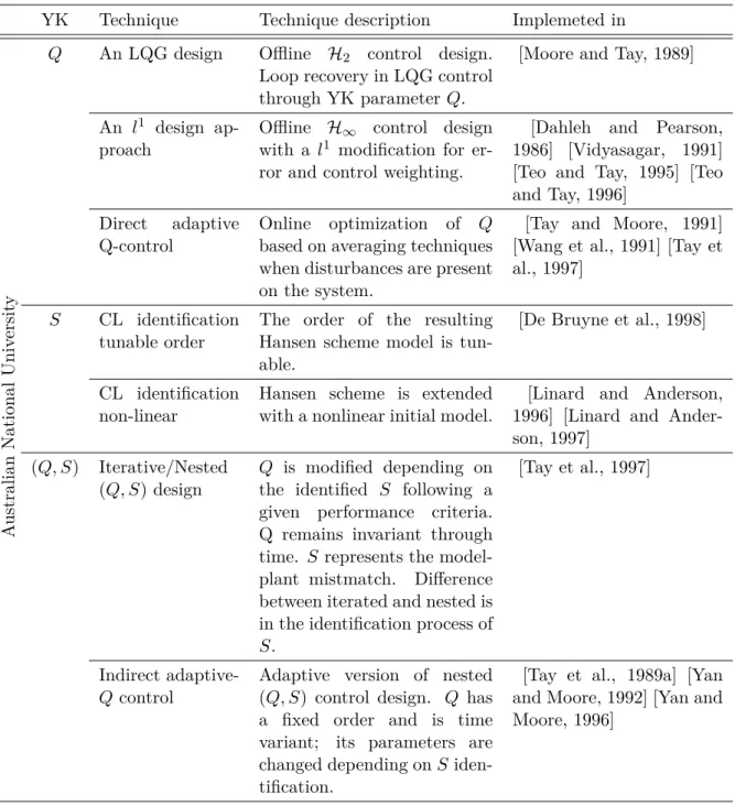
This chapter reviewed the YK control framework state-of-the art. Origins of the class of all stabilizing controllers for a plant K(Q), and its dual version, the class of all plants stabilized by a controller G(S) are explained. Robust stabilization results between Q and S are fundamental for the YK-based applications in the field of optimal, robust, adaptive and fault-tolerant control. These applications are mainly developed in three different institutions: Australian National University, Technical University of Denmark and Aalborg University. A state-of-the-art classification is in Table 2.1. YK applications timeline from the origin to the most recent work is in Fig. 2.2.
The Australian National University was the first to use YK parameterization as a control tool able to use classical control, optimal control, robust control and adaptive control theories together. High performance control goes beyond all of them by blending the strengths of each to obtain the best performance possible in a real world subject to uncertainties and system variations. Offline methods related to optimal LQG control and robust H∞control depending on Q are introduced to
achieve various performance objective. An adaptive version of the same is also proposed for cases where disturbances and uncertainties are not fully known. The dual YK parameterization plays a key role when unmodeled dynamics are present on the system. Iterative, nested and adaptive solutions consider the identified dynamics provided by S in order to optimize the YK filter Q. Theoretical basis present in [Tay et al., 1997] is strong and exemplified through simulation results for a hard disk servo system and a 55th order aircraft model. Experimental results with real applications are missing in the literature, especially for iterated/nested solutions. This is due to the degree explosion of the solution; with each iteration the order of the resulting parameters S and Q increase. Related also to the order, it looks complicated to get a simple representation of S even if the model-plant mistmath is simple. Order reduction techniques and model simplication should be carried out to make these solutions viables. There is neither an explicit parameterization
2.5. DISCUSSION 21 when considering decentralized control.
On the other hand, at the Technical University of Denmark, Professor Niemann extended the YK parameterization of all stabilzing controllers with additional sensors/actuators. This would be useful to solve decentralized and FTC problems. Research interests are dual YK parameter S description based on block uncertainty ∆. Several applications related to control optimization, performance and model validation are derived, but no simulation or experimental results are present in the literature. A YK-based fault tolerant control solution is also proposed, integrating controller reconfiguration, fault diagnosis and isolation in the same approach. The most advance FTC control architecture is in [Niemann, 2012]. Start-up or safe mode coexists with normal, full performance, reduced performance and closed-down modes. Fault detection based on dual YK parameterization determines which mode is applied through the corresponding Q. Safe mode is activated during start-up and fault isolation. Closed-down is set when the loop becomes irremediably unstable after a fault. Again, experimental real cases are missing.
University of Aalborg, through its project called Plug&Play control developed a novel con-cept for process distributed control, which allows the control system to self reconfigure once an instrumental change is introduced. The idea is similar to Niemann’s; in fact, an active collabora-tion exists between both universities. Extended version of YK parameterizacollabora-tion is crucial. While Niemann’s idea is more in the field of faults (a sensor or an actuator fails), here the objective is the opposite: a sensor or an actuator is plugged in, and the controller is reconfigured to enhance performance. An active collaboration between both should be set up in order to get a control system with full capabilities. Closed-down mode could be avoided if the correct sensor/actuator is plugged in. Simulation and experimental results well exemplified the application of the theory. It is by far, the part of the literature that presents more detailed and clear examples.
Once the state of the art of YK control framework has been carried out, current challenges are associated to the non-linear extension of the YK parameterization; integration of intelligent control system as fuzzy control, model predictive control, genetic algorithm or neuronal networks; transition analysis for the different YK-based control structures for switching in the literature; analysis of a scalar factor regulating the action between controllers through Q in order to improve the performance of the system; and extension of YK-based FTC and P&P to a more general control structure (they are all build with an observer-based feedback controller).
Different vehicles dynamics depending on longitudinal speed, emergency maneuvers in the sta-bility limit of pneumatic systems, or vibrations in chassis control are some examples of what a unique plant, as a vehicle, needs to handle through different control solutions. YK represents a suitable technique for its application in ITS. But, almost all the studied cases are mainly focused in system with very low dynamics, except from some simulation with an aircraft model in high perfor-mance control. There is neither a faster dynamics case, which in the case of ITS, sensor/actuators fails could result in a traffic accident. The application of YK in autonomous driving will not only serves as a tool, but as extension to real fast dynamics experimental cases.
![Table 3.1: CL poles (G, K α ). Direct linear change between K 0 and K 1 . α CL poles α = 0.0 [−998.67, −0.6660 ± 25.027i] α = 0.1 [−8.7288 ± 14.0935i, −0.6288 ± 25.0287i, −34.6057, −898.7287] α = 0.2 [−8.7279 ± 14.0891i, −0.5825 ± 25.0304i, −34.6244, −798.](https://thumb-eu.123doks.com/thumbv2/123doknet/2652283.60047/55.892.178.716.208.535/table-cl-poles-direct-linear-change-cl-poles.webp)