Learning conditionally lexicographic preference relations
Richard Booth
1, Yann Chevaleyre
2, J´erˆome Lang
2J´erˆome Mengin
3and Chattrakul Sombattheera
4Abstract. We consider the problem of learning a user’s ordinal pref-erences on a multiattribute domain, assuming that her prefpref-erences are lexicographic. We introduce a general graphical representation called LP-treeswhich captures various natural classes of such preference relations, depending on whether the importance order between at-tributes and/or the local preferences on the domain of each attribute is conditional on the values of other attributes. For each class we determine the Vapnik-Chernovenkis dimension, the communication complexity of preference elicitation, and the complexity of identify-ing a model in the class consistent with a set of user-provided exam-ples.
1
Introduction
In many applications, especially electronic commerce, it is impor-tant to be able to learn the preferences of a user on a set of alterna-tives that has a combinatorial (or multiattribute) structure: each al-ternative is a tuple of values for each of a given number of variables (or attributes). Whereas learning numerical preferences (i.e., utility functions) on multiattribute domains has been considered in various places, learning ordinal preferences (i.e., order relations) on multiat-tribute domains has been given less attention. Two streams of work are worth mentioning.
First, a series of very recent works focus on the learning of prefer-ence relations enjoying some preferential independencies conditions. Passive learning of separable preferences is considered by Lang & Mengin (2009), whereas passive (resp. active) learning of acyclic CP-nets is considered by Dimopoulos et al. (2009) (resp. Koriche & Zanuttini, 2009).
The second stream of work, on which we focus in this paper, is the class of lexicographic preferences, considered in Schmitt & Mar-tignon (2006); Dombi et al. (2007); Yaman et al. (2008). These works only consider very simple classes of lexicographic prefer-ences, in which both the importance order of attributes and the local preference relations on the attributes are unconditional. In this pa-per we build on these papa-pers, and go considerably beyond, since we consider conditionally lexicographic preference relations.
Consider a user who wants to buy a computer and who has a lim-ited amount of money, and a web site whose objective is to find the best computer she can afford. She prefers a laptop to a desktop, and this preference overrides everything else. There are two other at-tributes: colour, and type of optical drive (whether it has a simple DVD-reader or a powerful DVD-writer). Now, for a laptop, the next most important attribute is colour (because she does not want to be
1 University of Luxembourg. Also affiliated to Mahasarakham University,
Thailand as Adjunct Lecturer. [email protected]
2 LAMSADE, Universit´e Paris-Dauphine, France. {yann.chevaleyre,
lang}@lamsade.dauphine.fr
3IRIT, Universit´e de Toulouse, France. [email protected] 4Mahasarakham University, Thailand. [email protected]
seen at a meeting with the usual bland, black laptop) and she prefers a flashy yellow laptop to a black one; whereas for a desktop, she prefers black to flashy yellow, and also, colour is less important than the type of optical drive. In this example, both the importance of the attributes and the local preference on the values of some attributes may be conditioned by the values of some other attributes: the rel-ative importance of colour and type of optical drive depends on the type of computer, and the preferred colour depends on the type of computer as well.
In this paper we consider various classes of lexicographic prefer-ence models, where the importance relation between attributes and/or the local preference on an attribute may depend on the values of some more important attributes. In Section 2 we give a general model for lexicographic preference relations, and define six classes of lexico-graphic preference relations, only two of which have already been considered from a learning perspective. Then each of the following sections focuses on a specific kind of learning problem: in Section 3 we consider preference elicitation, a.k.a. active learning, in Sec-tion 4 we address the sample complexity of learning lexicographic preferences, and in Section 5 we consider passive learning, and more specifically model identification and approximation.
2
Lexicographic preference relations: a general
model
2.1
Lexicographic preferences trees
We consider a set A of n attributes. For the sake of simplicity, all attributes we consider are binary (however, our notions and results would still hold in the more general case of attributes with finite value domains). The domain of attribute X ∈ A is X = {x, x}. If U ⊆ A, then U is the Cartesian product of the domains of the attributes in U . Attributes and sets of attributes are denoted by upper-case Roman letters (X, Xi, A etc.). An outcome is an element of A; outcomes
are denoted by lower case Greek letters (α, β, etc.). Given a (partial) assignment u ∈ U for some U ⊆ A, and V ⊆ A, we denote by u(V ) the assignment made by u to the attributes in U ∩ V .
In our learning setting, we assume that, when asked to compare two outcomes, the user, whose preferences we wish to learn, is al-ways able to choose one of them. Formally, we assume that the (un-known) user’s preference relation on A is a linear order, which is a rather classical assumption in learning preferences on multi-attribute domains (see, e.g., Koriche & Zanuttini (2009); Lang & Mengin (2009); Dimopoulos et al. (2009); Dombi et al. (2007)). Allowing for indifference in our model would not be difficult, and most results would extend, but would require heavier notations and more details.
Lexicographic comparisons order pairs of outcomes (α, β) by looking at the attributes in sequence, according to their importance, until we reach an attribute X such that α(X) 6= β(X); α and β are
then ordered according to the local preference relation over the val-ues of X. For such lexicographic preference relations we need both an importance relation, between attributes, and local preference rela-tions over the domains of the attributes. Both the importance between attributes and the local preferences may be conditioned by the values of more important attributes. This conditionality can be expressed with the following class of trees:
Definition 1 A Lexicographic Preference Tree (or LP-tree) over A is a tree such that:
• every node n is labelled with an attribute Att(n) and a conditional preference tableCT(n) (details follow);
• every attribute appears once, and only once, on every branch; • every non-leaf node labelled with attribute Att(n) = X has
ei-ther one outgoing edge, labelled by{x, x}, or two outgoing edges, labelled respectively byx and x.
Domin(n) denotes the set of attributes labelling the ancestor nodes ofn, called dominating attributes for n. Domin(n) is partitioned be-tweeninstantiated attributes and non-instantiated attributes: Inst(n) (resp.NonInst(n)) is the set of attributes in Domin(n) that have two children (resp. that have only one child). Theconditional preference table associated with n consists of a subset U ⊆ NonInst(n) (the at-tributes on which the preferences onX depend) and for each u ∈ U , a conditional preference entry of the formu :>, where > is a linear order over the domain ofAtt(n). In our case, because the domains are binary, these rules will be of the formu : x > x or u : x > x. If U is empty, then the preference table is said to be maximally general and contains a single rule of the form> :>. If U = NonInst(n), then the preference table is said to bemaximally specific.
Note that since the preferences on a variable X can vary between branches, the preference on X at a given node n with Att(n) = X implicitly depends on the values of the variables in Inst(n). The only variables on which the preferences at node n do not depend are the ones that are less important that X.5
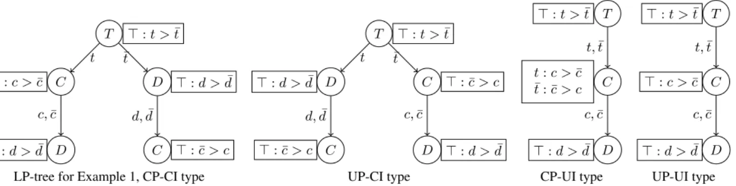
Example 1 Consider three binary attributes: C ( colour), with two values c (yellow) and c (black); D (dvd device) with two values d (writer) and d (read-only); and T (type) with values t (laptop) and t (deskop). On the first LP-tree depicted next page, T is the most im-portant attribute, with laptops unconditionally preferred to desktops; the second most important attribute is C in the case of laptops, with yellow laptops preferred to black ones, and D in the case of desk-tops. In all cases, a writer is always preferred to a read-only drive. The least important attribute is D for laptops, and C for desktops, black being preferred to yellow in this case.
If n is for instance the bottom leftmost leaf node, then Att(n) = D, Domin(n) = {T, C}, Inst(n) = {T } and NonInst(n) = {C}. 2 Definition 2 Given distinct outcomes α and β, and a node n of some LP-treeσ with X = Att(n), we say that n decides (α, β) if n is the (unique) node ofσ such that α(X) 6= β(X) and for every attribute Y in Domin(n), we have α(Y ) = β(Y ).
We defineα σ β if the node n that decides (α, β), is such that
CT(n) contains a rule u :> with α(U ) = β(U ) = u and α(X) > β(X), where u ∈ U for some U ⊆ NonInst(n) and X = Att(n). Proposition 1 Given a LP-tree σ, σis a linear order.
5Relaxing this condition could be interesting, but can lead to a weak relation
σ(see Def. 2): for instance, if we had attribute X more important than
Y , and local preferences on X depend on Y , e.g. y : x > ¯x ; ¯y : ¯x > x, one would not know how to compare xy and ¯x¯y.
Example 1 (continued) According to σ, the most preferred com-puters are yellow laptops with a DVD-writer, because cdt σ α
for any other outcome α 6= cdt; for any x ∈ C and any z ∈ D xzt σ xz¯t, that is, any laptop is preferred to any desktop
com-puter. And cd¯t σ c ¯¯d¯t, that is, a yellow deskop with DVD-writer
is preferred to a black one with DVD-reader because, although for desktops black is preferred to yellow, the type of optical reader is more important than the colour for desktop computers. 2 LP-trees are closely connected to Wilson’s “Pre-Order Search Trees” (or POST) (2006). One difference is that in POSTs, local pref-erence relations can be nonstrict, whereas here we impose linear or-ders, mainly to ease the presentation. More importantly, whereas in POSTs each edge is labelled by a single value, we allow more com-pact trees where an edge can be labelled with several values of the same variable; we need this because in a learning setting, the size of the representation that one learns is important.
2.2
Classes of lexicographic preference trees
Some interesting classes of LP-trees can be obtained by imposing a restriction on the local preference relations and/or on the condi-tional importance relation. The local preference relations can be con-ditional(general case), but can also be unconditional (the prefer-ence relation on the value of any attribute is independent from the value of all other attributes), and can also be fixed, which means that not only is it unconditional, but that it is known from the beginning and doesn’t have to be learnt (this corresponds to the distinction in Schmitt & Martignon (2006) between lexicographic strategies with or without cue inversion). Likewise, the attribute importance relation can be conditional (general case), or unconditional (for the sake of completeness, it could also be fixed, but this case is not very interest-ing and we won’t consider it any further). Without loss of generality, in the case of fixed local preferences, we assume that the local pref-erence on Xiis xi> xi.
Definition 3 (conditional/unconditional/fixed local preferences) • The class of LP-trees with unconditional local preferences (UP) is
the set of all LP-trees such that for every attributeXithere exists
a preference relation>i(eitherxi> xiorxi> xi) such that for
every noden with Att(n) = Xi, the local preference table atn is
> :>i.
• The class of LP-trees with fixed local preferences (FP) is the set of all LP-trees such that for every attributeXiand every noden
such thatAtt(n) = Xi, the local preference atn is xi> xi.
In the general case, local preferences can be conditional (CP). Obviously, FP ⊂ UP.
Definition 4 (conditional/unconditional importance) The class of LP-trees with anunconditional importance relation (UI) is the set of all linear LP-trees,i.e., for which every node n has only one child. In the general case, the importance relation can be conditional (CI). We stress that the class FP should not be confused with the class UP. FP consists of all trees where the local preference relation on each Xiis xi xi, while UP consists of all trees where the local
preference relation on each Xiis the same in all branches of the tree
(xi xior xi xi). For instance, if we have two variables X1, X2
and require the importance relation to be unconditional (UI) then we have only two LP-trees in FP-UI, whereas we have 8 in UP-UI.
T > : t > ¯t C t > : c > ¯c D c, ¯c > : d > ¯d D ¯ t > : d > ¯d C d, ¯d > : ¯c > c T > : t > ¯t D t > : d > ¯d C d, ¯d > : ¯c > c C ¯ t > : ¯c > c D c, ¯c > : d > ¯d T > : t > ¯t C t, ¯t t : c > ¯c ¯ t : ¯c > c D c, ¯c > : d > ¯d T > : t > ¯t C t, ¯t > : c > ¯c D c, ¯c > : d > ¯d
LP-tree for Example 1, CP-CI type UP-CI type CP-UI type UP-UI type
Figure 1. Examples of LP-trees
We can now combine a restriction on local preferences and a re-striction on the importance relation. We thus obtain six classes of LP-trees, namely, CP-CI, CP-UI, UP-CI, UP-UI, FP-CI and FP-UI. For instance, CP-UI is defined as the class of all LP-trees with condi-tional preferences and an uncondicondi-tional importance relation. The lex-icographic preferences considered in Schmitt & Martignon (2006); Dombi et al. (2007); Yaman et al. (2008) are all of the FP-UI or UP-UI type. Note that the LP-tree on Example 1 is of the CP-CI type. Examples of LP-trees of other types are depicted above.
3
Exact learning with queries
Our aim in this paper is to study how we can learn a LP-tree that fits well a collection of examples. We first consider preference elic-itation, a.k.a. active learning, or learning by queries. This issue has been considered by Dombi et al. (2007) in the FP-UI case (see also Koriche & Zanuttini (2009) who consider the active learning of CP-nets). The setting is as follows: there is some unknown target pref-erence relation >, and a learner wants to learn a representation of it by means of a lexicographic preference tree. There is a teacher, a kind of oracle to which the learner can submit queries of the form (α, β) where α and β are two outcomes: the teacher will then re-ply whether α > β or β > α is the case. An important question in this setting is: how many queries does the learner need in order to completely identify the target relation >? More precisely, we want to find the communication complexity of preference elicitation, i.e., the worst-case number of requests to the teacher to ask so as to be able to elicit the preference relation completely, assuming the target can be represented by a model in a given class. The question has al-ready been answered in Dombi et al. (2007) for the FP-UI case. Here we identify the communication complexity of eliciting lexicographic preferences trees in all five other cases, when all attributes are binary. (We restrict to the case of binary attributes for the sake of simplic-ity. The results for nonbinary attributes would be similar.) We know that a lower bound of the communication complexity is the log of the number of preference relations in the class. In fact, this lower bound is reached in all 6 cases:
Proposition 2 The communication complexities of the six problems above are as follows, when all attributes are binary:
FP UP CP
UI Θ(n log n) Dombi et al. (2007) Θ(n log n) Θ(2n)
CI Θ(2n) Θ(2n) Θ(2n)
Proof (Sketch) In the four cases FP-UI, UI, FP-CI and UP-CI, the local preference tables are independent of the structure of
the importance tree. There are n! unconditional importance trees, and Qn−1
k=0(n − k) 2k
conditional ones. Moreover, when prefer-ences are not fixed, there are 2n possible unconditional prefer-ence tables. For the CP-CI case, a complete conditional importance tree containsPn−1
k=02 k
= 2n− 1 nodes, and at each node there are two possible conditional preference rules. The elicitation pro-tocols of Dombi et al. (2007) for the UI-FP case can easily be extended to prove that the lower bounds are reached in the five other cases. For instance, for the FP-CI case, a binary search, us-ing log2n queries, determines the most important variable – for
example, with four attributes A, B, C, D the first query could be (ab¯c ¯d, ¯a¯bcd), if the answer were > we would know the most im-portant attribute is A or B; then for each of its possible values we apply the protocol for determining the second most important variable using log2(n − 1) queries, etc. When the local prefer-ences are not fixed, at each node a single preliminary query gives a possible preference over the domain of every remaining vari-able. We then get the following exact communication complexities:
FP UP CP
UI log(n!) n + log(n!) 2n− 1 + log(n!)
CI g(n) =
n−1
P
k=0
2klog(n − k) n + g(n) 2n− 1 + g(n) Finally, log(n!) = Θ(n log n) and g(n) = Θ(2n), from which the
table follows. 2
4
Sample complexity of some classes of LP-trees
We now turn to supervised learning of preferences. First, it is interest-ing to cast our problem as a classification problem, where the traininterest-ing data is a set of pairs of distinct outcomes (α, β), each labelled either > or < by a user: ((α, β), >) and ((α, β), <) respectively mean that the user prefers α to β, or β to α. (Recall that we assume that the user is always able to choose between two outcomes.). We want to learn a LP-tree σ that orders well the examples, e.g. such that α σ β for
every example ((α, β), >), and such that β σα for every example
((α, β), <). In this setting, the Vapnik-Chernovenkis (VC) dimen-sion of a class of LP-trees is the size of the largest set of pairs (α, β) that can be ordered correctly by some LP-tree in the class, whatever the labels (> or <) associated with each pair. In general, the higher this dimension, the more examples will be needed to correctly iden-tify a LP-tree.
Proposition 3 The VC dimension of any class of irreflexive, transi-tive relations over a set ofn binary attributes is strictly less than 2n
Proof (Sketch) Consider a set E of 2npairs of outcomes over A, and the corresponding undirected graph over A: it has as many edges as vertices, so it has at least one cycle; if all edges of this cycle are directed so as to obtain a directed cycle, the transitive closure of the corresponding relation over A will not be irreflexive. Hence E cannot be shattered with transitive irreflexive relations. 2 Proposition 4 The VC dimension of the class of CP-CI LP-trees and of CP-UI LP-trees overn binary attributes, is equal to 2n− 1. Proof (Sketch) It is possible to build a LP-tree over n attributes with 2knodes at the k − th level, for 0 ≤ i ≤ n − 1: this is a tree for CP-CI trees, it has 2n− 1 nodes. Such a tree can shatter a set of 2n− 1
examples: take one example for each node, the local preference rela-tion that is applicable at each node can be used to give both labels to the corresponding example. The upper bound follows from Prop. 3. 2
This result is rather negative, since it indicates that a huge number of examples would in general be necessary to have a good chance of closely approximating an unknown target relation. This important number of necessary examples also means that it would not be pos-sible to learn in reasonable - that is, polynomial - time. However, learning CP-CI LP-trees is not hopeless in practice: decision trees have a VC dimension of the same order of magnitude, yet learning them has had great success experimentally.
As for trees with unconditional preferences, Schmitt & Martignon (2006) have shown that the VC dimension of UP-UI trees over n binaryattributes is exactly n. Since every UP-UI tree is equivalent to a CP-UI tree, the VC dimension of UP-UI trees over n binary attributes is at least n.
5
Model identifiability
We now turn to the problem of identifying a model of a given class C, given a set E of examples. As before, an example is an ordered pair (α, β), meaning that the user prefers α to β – this is not restrictive since we assume that the user’s preference relation is a linear order. Definition 5 A LP-tree σ is said to be consistent with example (α, β) ifα σ β. Given a set of examples E, σ is consistent with E if it is
consistent with every example ofE.
The aim of the learner is to find some LP-tree in C consistent with E. Dombi et al. (2007) have shown that this problem can be solved in polynomial time for the class of binary LP-trees with unconditional importance and unconditional, fixed local preferences (FP-UI). In or-der to prove this, they exhibit a simple greedy algorithm that, given a set of examples E and a set P of unconditional local preferences for all attributes, outputs an importance relation on variables (that is, an LP-tree of the FP-UI class) consistent with E, provided there exists one. We will prove in this section that the result still holds for most of our classes of LP-trees, except one.
5.1
A greedy algorithm
We now present a generic algorithm able to generate LP-trees of various types. Given a set E of examples, algorithm 1 constructs a tree that satisfies the examples if such a tree exists, iteratively adding nodes from the root to the leaves. Depending on how the two func-tions chooseAttribute(n) and generateLabels(n, X) are defined,
Algorithm 1 GenerateLPTree
INPUT: A: set of attributes; E: set of examples over A; OUTPUT: LP-tree consistent with E, or FAILURE; 1. T ← {unlabelled root node};
2. while T contains some unlabelled node: (a) choose unlabelled node n of T ; (b) (X, CT ) ← chooseAttribute(n);
(c) if X = FAILURE then STOP and return FAILURE; (d) label n with X and CT ;
(e) L ← generateLabels(n, X); (labels for edges below n) (f) for each l ∈ L:
add new unlabelled node to T , attached to n with edge labelled with l;
3. return T .
the output tree will have conditional/unconditional/fixed preference tables, and conditional/unconditional attribute importance.
At a given currently unlabelled node n, step 2b considers the set E(n) = {(α, β) ∈ E | α(Domin(n)) = β(Domin(n))}, that is, the set of all examples in E for which α and β coincide on all variables above Att(n) in the branch from the root to n. E(n) is the set of examples that correspond to the assignments made in the branch so far and that are still undecided. The helper function chooseAttribute(n) returns an attribute X /∈ Domin(n) and a con-ditional table CT . Informally, the attribute and the local preferences are chosen so that they do not contradict any example of E(n): for every (α, β) ∈ E(n), if α(X) 6= β(X) then CT must contain a rule of the form u : α(X) > β(X), with u ∈ U , U ⊆ NonInst(n) and α(U ) = β(U ) = u. If we allow the algorithm to generate conditional preference tables, the function chooseAttribute(n) may output any (X, CT ) satisfying the above condition. However, if we want to learn a tree with unconditional or fixed preferences we need to impose appropriate further conditions; we will say (X, CT ) is: UP-choosable if CT is of the form > :> (a single unconditional
rule);
FP-choosable if CT is of the form > : x > ¯x.
If no attribute can be chosen with an appropriate table without contra-dicting one of the examples, chooseAttribute(n) returns FAILURE and the algorithm stops at step 2c.
Otherwise, the tree is expanded below n with the help of the func-tion generateLabels, unless Domin(n) ∪ {X} = A, in which case n is a leaf and generateLabels(n, X) = ∅. If this is not the case, generateLabels(n, X) returns labels for the edges below the node just created: it can return two labels {{x} and {¯x}} if we want to split with two branches below X, or one label {x, ¯x} when we do not want to split. If we want to learn a tree of the UI class, clearly we never split. If we want to learn a tree with possible conditional im-portance, we create two branches, unless the examples in E(n) that are not decided atn all have the same value for X, in which case we do not split. An important consequence of this is that the number of leaves of the tree built by our algorithm never exceeds |E|.
5.2
Some examples of GenerateLPTree
Throughout this subsection we assume the algorithm checks the at-tributes for choosability in the order T → C → D.
1: (tcd, t¯cd); 2: (¯t¯cd, ¯tcd); 3: (tc ¯d, t¯c ¯d); 4: (¯t¯c ¯d, ¯tc ¯d); 5: (¯t¯cd, ¯tc ¯d) Let’s try using the algorithm to construct a UP-UI tree consistent with E. At the root node n0of the tree we first check if there is table
CT such that (T, CT ) is choosable. By the definition of UP-choosability, CT must be of the form {> :>} for some total order > of {t, ¯t}. Now since α(T ) = β(T ) for all (α, β) ∈ E(n0) = E,
(T, {> :>}) is choosable for any > over {t, ¯t}. Thus we label n0
with e.g. T and > : t > ¯t (we could have chosen > : ¯t > t instead). Since we are working in the UI-case the algorithm generates a single edge from n0 labelled with {t, ¯t} and leading to a new unlabelled
node n1. We have E(n1) = E(n0) since no example is decided at n0.
So C is not UP-choosable at n1, owing to the opposing preferences
over C exhibited for instance in examples 1,2. However (D, {> : d > ¯d}) is UP-choosable, thus the algorithm labels n1 with D and
{> : d > ¯d}. Example 5 is decided at n1. At the next node the only
remaining attribute C is not UP-choosable because for instance we still have 1,2 ∈ E(n2). Thus the algorithm returns FAILURE. Hence
there is no UP-UI tree consistent with E.
However, if we allow conditional preferences, the algorithm does successfully return the CP-UI tree depicted on Fig. 1, because C is choosable at node n1, with the conditional table {t : c > ¯c ; ¯t : ¯c > c}.
All examples are decided at n0or n1, and the algorithms terminates
with an arbitrary choice of table for the last node, labelled with D.2 This example raises a couple of remarks. Note first that the choice of T for the root node is really a completely uninformative choice in the UP-UI case, since it does not decide any of the examples. In the CP-UI case, the greater importance of T makes it possible to have the local preference over C depend on the values of T . Second, in the CP-UI case, the algorithm finishes the tree with an arbitrary choice of table for the leaf node, since all examples have been de-cided above that node; this way, the ordering associated with the tree is complete, which makes the presentation of our results easier. In a practical implementation, we may stop building a branch as soon as all corresponding examples have been decided, thus obtaining an incomplete relation.
Example 3 Consider now the following examples:
1: (tcd, t¯cd); 2b: (tcd, tc ¯d); 3b: (¯tcd, ¯t¯c ¯d); 4: (¯t¯c ¯d, ¯tc ¯d); 5: (¯t¯cd, ¯tc ¯d) We will describe how the algorithm can return the CP-CI tree of Ex. 1, depicted on Fig. 1, if we allow conditional importance and preferences. As in the previous example, T is CP-choosable at the root node n0 with a preference table {> : t > ¯t}. Since we are
now in the CI-case, generateLabels generates an edge-label for each value t and ¯t of T . Thus two edges from n0are created, labelled with
t, ¯t resp., leading to two new unlabelled nodes m1and n1.
We have E(m1) = {(α, β) ∈ E | α(T ) = β(T ) = t} = {1, 2b},
so chooseAttribute returns (C, {> : c > ¯c}), and m1 is labelled
with C and > : c > ¯c. Since only example 2b remains undecided at m1, no split is needed, one edge is generated, labelled with {c, ¯c},
leading to new node m2 with E(m2) = {2b}. The algorithm
suc-cessfully terminates here, labelling m2with D and > : d > ¯d.
On the other branch from n0, we have E(n1) = {3b, 4, 5}. Due
to the opposing preferences on their restriction to C exhibited by examples 3b,5, C is not choosable. Thus we have to consider D instead. Here we see that (D, {> : d > ¯d}) can be returned by chooseAttribute thus n1is labelled with D, and > : d > ¯d. The only
undecided example that remains on this branch is 4, so the branch is finished with a node labelled with C and > : ¯c > c. 2
5.3
Complexity of model identification
The greedy algorithm above solves five learning problems. In fact, the only problem that cannot be solved with this algorithm, as will be shown below, is the learning of a UP-CI tree without initial knowl-edge of the preferences.
Proposition 5 Using the right type of labels and the right choosabi-lity condition, the algorithm returns, when called on a given setE of examples, a tree of the expected type, as described in the table below, consistent withE, if such a tree exists:
learning problem chooseAttribute generateLabels CP-CI no restriction split possible CP-UI no restriction no split
UP-UI UP-choosable no split
FP-CI FP-choosable split possible
FP-UI FP-choosable no split
Proof (Sketch) The fact that the tree returned by the algorithm has the right type, depending on the parameters, and that it is consistent with the set of examples is quite straightforward. We now give the main steps of the proof of the fact that the algorithm will not return failure when there exists a tree of a given type consistent with E.
Note first that given any node n of some LP-tree σ, labelled with X and the table CT, then (X, CT ) is candidate to be returned by chooseAttribute. So if we know in advance some LP-tree σ consis-tent with a set E of examples, we can always construct it using the greedy algorithm, by choosing the “right” labels at each step.
Importantly, it can also be proved that if at some node n chooseAttribute chooses another attribute Y , then there is some other LP-tree σ0, of the same type as σ, that is consistent with E and extends the current one; more precisely, σ0is obtained by mod-ifying the subtree of σ rooted at n, taking up Y to the root of this subtree. Hence the algorithm cannot run into a dead end. 2 This result does not hold in the UP-CI case, because taking an attribute upwards in the tree may require using a distinct preference rule, which may not be correct in other branches of the LP-tree. Example 4 Consider now the following examples:
1b: (tcd, t¯c ¯d); 2b: (tcd, tc ¯d); 4b: (¯t¯c ¯d, ¯tcd); 5: (¯t¯cd, ¯tc ¯d) The UP-CI tree depicted on Fig. 1 is consistent with {1b, 2b, 4b, 5}. However, if we run the greedy algorithm again, trying this time to en-force unconditional preferences, it may, after labelling the root node with T again, build the t branch first: it will choose C with prefer-ence > : c > ¯c and finish this branch with (D, > : d > ¯d); when building the ¯t branch, it cannot choose C first, because the preference has already been chosen in the t branch and would wrongly decide 5; but D cannot be chosen either, because 4b and 5 have opposing
preferences on their restrictions to D. 2
Proposition 6 The problems of deciding if there exists a LP-tree of a given class consistent with a given set of examples over binary attributes have the following complexities:
FP UP CP
UI P(Dombi et al. , 2007) P P
CI P NP-complete P
Proof (Sketch) For the CP-CI, CP-UI, FP-CI, FP-UI and UP-UI cases, the algorithm runs in polynomial time because it does not have
more than |E| leaves, and each leaf cannot be at depth greater than n; and every step of the loop except (2b) is executed in linear time, whereas in order to choose an attribute, we can, for each remaining attribute X, consider the relation {(α(X), β(X)) | (α, β) ∈ E(n)} on X: we can check in polynomial time if it has cycles, and, if not, extend it to a total strict relation over X.
For the UP-CI case, one can guess a set of unconditional local preference rules P , of size linear in n, and then check in polyno-mial time (FP-CI case) if there exists a tree T such that (T, P ) is consistent with E; thus the problem is in NP. Hardness comes from a reduction fromWEAK SEPARABILITY– the problem of checking if there is a CP-net without dependencies weakly consistent with a given set of examples – shown to be NP-complete by Lang & Men-gin (2009). More precisely, a set of examples E is weakly separable if and only if there exists a (non ambiguous) set of unconditional preference rules that contains, for every (α, β) ∈ E, a rule X, > :> such that α(X) > β(X). To prove the reduction, given a set of ex-amples E = {(α1, β1), . . . , (αm, βm)}, built on a set of attributes
{X1, . . . , Xn}, we introduce m new attributes P1, . . . , Pm. For each
example ei= (αi, βi) ∈ E we create a new example
e0i= (αip1. . . pi−1pipi+1. . . pm, βip1. . . pi−1pipi+1. . . pm).
If E is weakly separable, we can build a UP-CI LP-tree consistent with E0 = {e0i | ei ∈ E}: the m top levels of the tree are labelled
with the Pis; below that there remains no more that one example on
each branch, and the importance order on that branch can be chosen to decide well the corresponding example. For the converse, it is not hard to see that the restriction to X1, . . . , Xnof the tables of a UP-CI
tree consistant with E0is weakly compatible with E. 2
5.4
Complexity of model approximation
In practice, it is often the case that no structure of a given type is con-sistent with all the examples at the same time. It is then interesting to find a structure that is consistent with as many examples as possible. In the machine learning community, the associated learning problem is often refered to as agnostic learning. Schmitt & Martignon (2006) have shown that finding a UI-UP LP-tree, with a fixed set of local preferences, that satisfies as many examples from a given set as pos-sible, is NP-complete, in the case where all attributes are binary. We extend these results here.
Proposition 7 The complexities of finding a LP-tree in a given class, which wrongly classifies at mostk examples of a given set E of ex-amples overbinary attributes, for a given k, are as follows:
FP UP CP
UI NP-c. (Schmitt & Martignon (2006)) NP-c. NP-c.
CI NP-c. NP-c. NP-c.
Proof (Sketch) These problems are in NP because in each case a witness is the LP-tree that has the right property, and such a tree need not have more nodes than there are examples. For the UP-CI case, the problem is already complete for k = 0, so it is hard. NP-hardness of the other cases follow from successive reductions from the case proved by Schmitt & Martignon (2006). 2
6
Conclusion and future work
We have proposed a general, lexicographic type of models for repre-senting a large family of preference relations. We have defined six in-teresting classes of models where the attribute importance as well as the local preferences can be conditional, or not. Two of these classes
correspond to the usual unconditional lexicographic orderings. Inter-estingly, classes where preferences are conditional have an exponen-tional VC dimension.
We have identified the communication complexity of the five classes for which it was not previously known, thereby generalizing a previous result by Dombi et al. (2007).
As for passive learning, we have proved that a greedy algorithm like the ones proposed by Schmitt & Martignon (2006); Dombi et al. (2007) for the class of unconditional preferences can identify a model in another four classes, thereby showing that the model identification problem is polynomial for these classes. We have also proved that the problem is NP-complete for the class of models with conditional at-tribute importance but unconditional local preferences. On the other hand, finding a model that minimizes the number of mistakes turns out to be NP-complete in all cases.
Our LP-trees are closely connected to decision trees. In fact, one can prove that the problem of learning a decision tree consistent with a set of examples can be reduced to a problem of learning a CP-CI LP tree. It remains to be seen if CP-CI trees can be as efficiently learnt in practice as decision trees.
In the context of machine learning, usually the set of examples to learn from is not free of errors in the data. Our greedy algorithm is quite error-sensitive and therefore not robust in this sense; it will even fail in the case of a collapsed version space. Robustness toward errors in the training data is clearly an important property of real world applications.
As future work, we intend to test our algorithms, with appropri-ate heuristics to guide the choice of variables a each stage. A possi-ble heuristics would be the mistake rate if some unconditional tree is built below a given node (which can be very quickly done). An-other interesting aspect would be to study mixtures of conditional and unconditional trees, with e.g. the first two levels of the tree being conditional ones, the remaining ones being unconditional (since it is well-known that learning decision trees with only few levels can be as good as learning trees with more levels).
Acknowledgements We thank the reviewers for very helpful com-ments. This work has received support from the French Ministry of Foreign Affairs and the Commission on Higher Education, Ministry of Education, Thailand. A preliminary version of this paper has been presented the Preference Learning workshop 2009.
References
Dimopoulos, Y., Michael, L., & Athienitou, F. 2009. Ceteris Paribus Preference Elicitation with Predictive Guarantees. Proc. IJCAI’09, pp 1890-1895.
Dombi, J., Imreh, C., & Vincze, N. 2007. Learning Lexicographic Orders. European J. of Operational Research, 183, pp 748–756. Koriche, F., & Zanuttini, B. 2009. Learning conditional preference
networks with queries, Proc. IJCAI’09, pp 1930-1935.
Lang, J., & Mengin, J. 2009. The complexity of learning separable ceteris paribus preferences. Proc. IJCAI’09, pages 848-853. Schmitt, M., & Martignon, L. 2006. On the Complexity of Learning
Lexicographic Strategies. J. of Mach. Learning Res., 7, pp 55–83. Wilson, N. 2006. An Efficient Upper Approximation for Conditional
Preference. In Proc. ECAI 2006, pp 472-476.
Yaman, F., Walsh, T., Littman, M., & desJardins, M., 2008. Demo-cratic Approximation of Lexicographic Preference Models. In: Proc. ICML’08, pp 1200-1207.