Laboratoire d'Analyse et Modélisation de Systèmes pour l'Aide à la Décision CNRS UMR 7243
CAHIER DU LAMSADE
309
Mai 2011
A cartography of spacial relationships in a symbolic
image database
LAMSADE Research Report n
◦XXX
A cartography of spatial relationships in a symbolic image database
Nguyen Vu Hoang1,2, Valérie Gouet-Brunet2, Marta Rukoz1,3
1 : LAMSADE - Université Paris-Dauphine - Place de Lattre de Tassigny - F75775 Paris Cedex 16 2 : CEDRIC/CNAM - 292, rue Saint-Martin - F75141 Paris Cedex 03
3 : Université Paris Ouest Nanterre La Défense - 200, avenue de la République - F92001 Nanterre Cedex [email protected], [email protected] , [email protected]
18 avril 2011
Abstract
This work addresses the problem of the representation of spatial relationships between sym-bolic objects in images. We have studied the distribution of several categories of relationships in LabelMe1, a public database of images where objects are annotated manually and online by users. Our objective is to build a cartography of the spatial relationships that can be encountered in a representative database of images of heterogeneous content, with the main aim of exploiting it in future applications of Content-Based Image Indexing (CBIR), such as object recognition or retrie-val. In this paper, we present the framework of the experiments made and give an overview of the main results obtained, as an introduction to the website1dedicated to this work, whose ambition is to make available all these statistics to the CBIR community.
1
Introduction
We are interested in the representation of spatial relationships between symbolic objects in images. In CBIR, embedding such information into image content description provides a better representation of the content as well as new scenarios of interrogation. Literature on spatial relationships is very rich -several hundreds of papers exist on this topic - and a lot of approaches were proposed (see for example the survey [4]). Most of them describe different aspects of spatial relationships, e.g. directional [7] or topological [3] relationships, and have been evaluated on small synthetic or specific image datasets, e.g. medical or satellite imagery. In this work, we propose to build a cartography of the spatial relationships that can be encountered in a database of images of heterogeneous natural contents, such as audiovi-sual, web or family visual contents. We have chosen a public annotated database, from the platform
LabelMe1
, which is described in section 2. This cartography collects statistical informations on the trends of spatial relationships involving symbolic objects effectively encountered in this database, with
the aim of exploiting them in future CBIR applications, for improving tasks such as object recognition or retrieval. Here, we focus on the analysis of unary, binary, and ternary relationships. We present the results of this analysis, which are made available to the CBIR community on our website2
.
This report is organized as follows : In Section 2, we introduce the LabelMe image database used in our work and objects categories extracted from it. Section 3, 4, and 5 are respectively dedicated to the statistical studies on unary, binary and ternary relationship. Finally, a conclusion of this work to finish the report is presented in Section 6.
2
Annotated image database
2.1 Studied database
LabelMe [12] is a platform containing image databases and an online annotation tool that allows users to indicate freely, by constructing a polygon and a label, the many objects depicted in a image as they wish. Thus, each object, called entity in this work, is presented by a polygon and a label. In our work, each label is considered as the name of an entity category, so all entities possessing the same label belong to a same category. We used one of the test databases of this platform which contains 1133 annotated images in daily contexts (see examples in Fig.1 and Fig.2). The content of these images is very heterogeneous, it contains many categories and many images, and it is not specific to a particular domain. Therefore, studying this database can provide a general view about categories and their relationships, and the results should not be influenced noticeably by changing the database. In order to guarantee the quality of the database we verified carefully each annotated image for consistency :
– Firstly, we manually consolidated synonymous labels by correcting orthographic mistakes and merging labels having the same meaning.
– Secondly, we identified and selected 86 different categories in taking into account only ones having at least 15 occurrences. This decision was taken to ensure an independence of statistical results even whether the image database is changed. These 86 categories are listed in Table 1 ordered by category’s label and in Table 2 ordered by category’s id .
– Lastly, we added missing annotations to entities of the considered categories, except for too small size entities or entities belonging to a category having a high frequency of already annotated entities in the image, such as "leaf", "window", "flower", etc. In this way, the statistical results should not be biased by these missing annotations.
In the rest of the paper, we call DB this database. Now, we can ensure that the set of entities annotated in DB contains all the interesting entities that attract human attention view. Thus, this new annotated image database has a higher quality than the original one. Before beginning this work, we formulate two different hypotheses :
– The set of entities annotated in DB contains all the interesting objects that the photographer
wants to present.
– The entities annotated are the ones attracting most attention view of LabelMe’s annotators, and contain a subset of interesting objects that the photographer wants to present.
Sometimes, the viewpoint of a photographer is different from public’s one. That means the subject annotated can be different from the photographer’s intention. Consequently, the statistical results would depend on annotations of LabelMe’s users. With the original database, the second hypothesis can represents a useful dataset for a study on human attention view. After a verification and a consolidation, we think that first hypothesis is verified with DB.
Figure 1 – Images of DB.
Sky, tree, person, lake, ground Road,car, building, window Sky,tree, mountain, ground
Figure 2 – Images of DB with their polygons and associated annotations.
2.2 Statistics on categories
Before studying different relationships between categories, we take a look at statistics concerning each category, for example, its highest and lowest numbers of entities in an image, the total number of its entities in DB, the number of images where at less one of its entities appears, etc. This statistical study is presented in Table 3. A overview of these statistics is presented in Table 4.
Category label Category ID Category label Category ID Category label Category ID
air conditioning 21 fire-hydrant 46 pot 40
arm 65 flag 47 railing 28
attic 73 flower 55 road 09
awning 60 grass 43 rock 22
balcony 44 grille 29 roof 14
bench 48 ground 17 sand 69
bicycle 58 handrail 31 sculpture 81
billboard 78 hat 86 sea 71
bird 76 head 63 sidewalk 06
blind 27 headlight 30 sign 12
block 82 lake 74 sky 10
boat 70 lamp 33 stair 24
box 41 leaf 83 street-light 16
building 05 license plate 07 table 67
bus 61 light 39 tail light 19
car 02 mailbox 54 text 49
chair 50 manhole 23 torso 64
chimney 08 mast 79 traffic light 53
clock 62 mirror 18 tree 04
cloud 80 motorbike 77 truck 38
column 34 mountain 84 umbrella 68
cone 66 pane 35 van 37
crosswalk 59 parking-meter 51 wall 11
curb 52 path 56 water 72
door 25 person 36 wheel 26
duck 75 pipe 42 window 01
fence 03 plant 13 wind-shield 32
field 85 pole 15 wire 20
fire escape 45 poster 57
Table 1 – 86 entity categories in DB, ordered by label.
From Table 3, we can see that the average entities number of each category in an image could be used to have a quick view about the possibility of having more than one of its entities in an image. For example, category 1 (window) has a high number of occurrences in DB and its average is around 19 entities per image. That means that, if we find a window in an image, we can expect to find another window in the same image. Category 82 (block) has a considerable average also, around 10.25 entities per image. Meanwhile, some categories, like lake or sun, do not have more than one entity per image. Certainly, it is not current to have two entities of lake in an image, and it is evident that there is only one sun in the sky. Note that, because of a low number of occurrences of sun in DB, we did not take into account this category in DB.
Interpretation with averages can provide quickly a general information on categories, but we can do it better. For a more detailed study, we have computed the intra-class correlation of categories, based on the classic correlation function between two categories. For a category, the inter-class correlation
Category label Category ID Category label Category ID Category label Category ID
window 01 headlight 30 crosswalk 59
car 02 handrail 31 awning 60
fence 03 wind-shield 32 bus 61
tree 04 lamp 33 clock 62
building 05 column 34 head 63
sidewalk 06 pane 35 torso 64
license plate 07 person 36 arm 65
chimney 08 van 37 cone 66
road 09 truck 38 table 67
sky 10 light 39 umbrella 68
wall 11 pot 40 sand 69
sign 12 box 41 boat 70
plant 13 pipe 42 sea 71
roof 14 grass 43 water 72
pole 15 balcony 44 attic 73
street-light 16 fire escape 45 lake 74
ground 17 fire-hydrant 46 duck 75
mirror 18 flag 47 bird 76
tail light 19 bench 48 motorbike 77
wire 20 text 49 billboard 78
air conditioning 21 chair 50 mast 79
rock 22 parking-meter 51 cloud 80
manhole 23 curb 52 sculpture 81
stair 24 traffic light 53 block 82
door 25 mailbox 54 leaf 83
wheel 26 flower 55 mountain 84
blind 27 path 56 field 85
railing 28 poster 57 hat 86
grille 29 bicycle 58
Table 2 – 86 entity categories in DB, ordered by id.
function is defined as : cor(x, y) = σxy σxσy (1) = N X i=1 (xi− ¯x) · (yi− ¯y) v u u t N X i=1 (xi− ¯x)2· v u u t N X i=1 (yi− ¯y)2 (2)
N is the number of images in DB. For a category Cj, every first entity found in an image is conside-red as variable x, another entity as variable y. Therefore, ¯x and ¯y are their average occurrence number in DB. In image Ii, if there is only one entity of Cj, then xi = 1 and yi = 0. If there are more than two entities, then xi = 1 and yi = 1. Otherwise, xi = 0 and yi = 0.
cate-Categ. Highest Average Nb of Num of Categ. Highest Average NB of Num of
ID nb of occ. in img. ID nb of occ. in img.
occ. in all DB where occ. in all DB where
an img categ. an img categ.
presents presents 01 177 19.64 13297 677 02 31 4.59 2382 519 36 75 4.65 2295 494 05 32 2.75 2145 780 04 21 2.79 1758 630 26 13 4.03 1462 363 06 6 1.83 1123 614 12 11 2.28 964 423 25 8 2.04 822 403 10 4 1.11 821 740 09 4 1.16 744 641 13 8 1.81 615 340 16 11 1.7 564 331 27 45 7.31 446 61 15 17 1.92 435 226 65 26 4.05 421 104 44 24 3.41 395 116 07 4 1.42 352 248 32 5 1.67 345 206 30 8 1.82 298 164 18 4 1.42 295 208 64 20 2.89 292 101 63 18 2.67 288 108 19 6 1.71 286 167 60 12 2.23 252 113 49 6 1.62 248 153 43 5 1.5 246 164 58 7 1.83 218 119 34 20 3.1 214 69 11 4 1.36 202 149 35 14 3.1 195 63 03 5 1.43 192 134 53 5 1.87 189 101 24 5 1.34 155 116 21 11 1.8 142 79 33 12 2.22 140 63 28 7 1.73 126 73 31 7 1.97 124 63 23 5 1.4 120 86 55 5 1.52 111 73 51 4 1.42 109 77 84 5 1.39 106 76 29 9 2.43 102 42 47 6 1.63 96 59 70 18 3.67 88 24 17 3 1.14 82 72 57 10 1.88 75 40 76 11 1.4 73 52 14 5 1.43 73 51 40 4 1.61 71 44 73 19 3.33 70 21 48 5 1.79 68 38 83 9 2.16 67 31 56 3 1.16 67 58 37 5 1.26 67 53 22 14 2.78 64 23 59 3 1.17 61 52 50 18 3.05 61 20 08 3 1.33 60 45 38 3 1.26 58 46 72 2 1.08 55 51 46 3 1.07 48 45 42 5 1.31 46 35 68 7 2.15 43 20 82 20 10.25 41 4 52 3 1.21 41 34 75 9 3 36 12 71 3 1.06 35 33 67 15 2.33 35 15 54 4 1.4 35 25 61 3 1.13 34 30 39 5 2.06 33 16 86 32 32 32 1 80 5 1.52 32 21 78 5 1.36 30 22 69 2 1.17 28 24 41 4 1.22 28 23 81 10 1.93 27 14 20 7 2.45 27 11 85 3 1.44 26 18 66 4 1.47 25 17 62 2 1.05 23 22 79 4 1.57 22 14 77 3 1.31 21 16 45 4 1.9 19 10 74 1 1 16 16
Table 3 –Categories’ statistics in DB.
gory’s appearance on another, the intra-class correlation is never negative. Returning to the previous examples, we obtained 0.776 for the intra-class correlation of windows, that is also the highest score among intra-class correlations obtained. This score is high enough to conclude that we can find mostly at least twowindows in an image where a windows entity has already detected. The lowest score
Nb of Nb of Average of Average of Max. nb of Min. nb of
img/DB entities/DB entities/cat.(STDEV) entities/img (STDEV) entities/img entities/img
1133 38075 442.7 (1485.6) 33.6 (32.3) 264 1
Table 4 –Statistical overview of DB.
in this study is 0, related to lake category. Therefore, no image in DB contains more than a lake. In fact, it is not usual to have two or more instances of lake in the same image. Summarizing, 21 categories have intra-class correlation higher than 0.3 while only 8 categories have a score higher than 0.5, for example car, window, building (view histograms of inter-class correlation in Fig.3 and for more details, view Tab.16 in Annex A.1).
Figure 3 – Histogram of inter-class correlation of categories in DB.
This study can provide useful information in the category detection process, if we want, for example, to detect all entities of a category Ci present in an image I. Knowing that Ci has, in general, one en-tity per image (based on a threshold on correlation, for example), as soon as the first enen-tity of Ci is detected, we could finish the detection process, thus reducing significantly the execution time of the detection. The statistics for all categories are available on our website2.
In the next sections, we present a discuss of the statistical results on three different types of relationships : unary, binary and ternary relationships.
3
Unary relationships
3.1 Representation
We call unary relationship, the relationship between an entity and its localization in an image, where localization is defined as a region or area of the image, represented in this work by a code. More formally, let A = {Ai}, I = {Ij}, and C = {Ck} be the set of areas, the set of images, and the set of categories, respectively. The unary relationship is an application R from C × I to A. R(Ck, Ij) ∈ A allows knowing where Ck is located in Ij.
Areas of an image can be represented in different ways like quad-tree or quin-tree, see for example [11, 13]. Since we do not have any knowledge a priori of the location of the categories in the images, we propose to split images in a fixed number of regular areas (i.e. equal size areas). First, we divide each image in a fixed sized grid. Each cell of this grid, called atomic area, is represented by a code. Fig.4 and 5 depict a splitting in 9 or in 16 different basic areas and theirs codes, respectively. We then combine these codes to present more complex areas, by example for 9-area splitting, code 009 represents area ( ) grouping together areas 001( ) and 008( ).
001 008 064 002 016 128 004 032 256
Figure 4 –Codes in unary relationship by splitting an image in nine areas.
00001 00016 00256 04096 00002 00032 00512 08192 00004 00064 01024 16384 00008 00128 02048 32768
Figure 5 –Codes in unary relationship by splitting an image in 16 areas.
3.2 Results analysis
The combination of nine 9-area splitting codes (Fig.4) gives 511 possible atomic/complex area codes. However, some codes could not be used, for example, code 017 ( ) or code 161 ( ) because their atomic areas are not connected by an edge (i.e. they are disjoint). It is impossible to have locations occupied by an entity in this way. In consequence, based on this idea, there are only 218 theoretically authorized codes (see the recursive algorithm to create theoretically authorized codes from a set of atomic codes in equation 16 of Annex B.1). Concretely, in DB, we did not find any entity in areas represented by impossible codes. Moreover, there are only 138 useful theoretically authorized codes, meaning that 80 codes are not encountered in DB. For example, DB does not contain any entity in areas with codes 47( ) or 125 ( ). In the same way, the combination of 16 codes in Fig.5 gives us 65535 different codes. In theory, we can reach 11506 atomic/complex areas (based on connected areas), but in DB, only 649 codes are present.
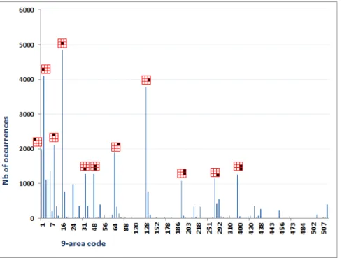
Figure 6 – Distribution of 9-area splitting codes.
Figure 7 – Distribution of 16-area splitting codes.
Figure 8 – Number of categories according to 9-area splitting codes.
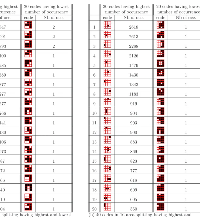
For each type of splitting, we could retrieve easily number of occurrence or distribution of categories by report of their codes (view Fig.6 and 8 for 9-area splitting, Fig.7 and 9 for 16-area splitting). Some codes having the highest or lowest number of occurrences are reported in Table 5. In Annex B.1, Fig. 34 and 33 illustrate the distribution of categories according to two 9-area codes : 16( -code having highest frequency) and 128( -code concerning the most number of categories). Fig.36 and 35 represent a such distribution in 16-area splitting for codes 1024( ) and 16384( ). These informations provided us some interesting information to interpret the trend of categories’location in image.
3.3 Interpretation
From the Fig.6 and 7, we can observe that on the one hand, that large or complex regions have a small number of occurrences. That means that object categories are mostly represented by a simple and small area. On the other hand, the trend of the categories’ presence, in first, is on the middle line, then, on the second line, and finally on a combination of the second and the third lines. In fact, it is not usual to present an interesting object only on the bottom line. And in practice, this line does not attract also the attention view. Similarly, we can observe that the trend of the categories’ presence, on the left is higher than on the right. These conclusions confirm the well known rules concerning photography and ergonomics (human-computer interaction) :
Figure 9 – Number of categories according to 16-area splitting codes.
– In photography, there is the rule of thirds3
, one of the first rules of composition taught to most photography students. An image is cut by two horizontal lines and two vertical lines. It is recommended to present interesting object in the intersections or along the lines presented in this rule (see Fig.10).
Figure 10 – Horizontal and vertical lines in rule of thirds in photography.
– According to [8, 10] concerning ergonomic studies on human-computer interaction, the center of computer screen is the most attracting. Next, the human attention view is attracted by the top and the left of screen more than by the bottom and the right consecutively, leading to slightly more annotated entities in these areas.
We have studied the distribution of categories across areas of the image, according to 9-area and 16-area splittings. Basically, the results obtained can be encapsulated in a knowledge-based system
20 codes having highest 20 codes having lowest number of occurrence number of occurrence code Nb of occ. code Nb of occ.
1 4847 2 2 4091 2 3 3793 2 4 2100 1 5 1985 1 6 1889 1 7 1377 1 8 1277 1 9 1277 1 10 1266 1 11 1141 1 12 1130 1 13 1106 1 14 1073 1 15 987 1 16 772 1 17 766 1 18 540 1 19 410 1 20 404 1
20 codes having highest 20 codes having lowest number of occurrence number of occurrence code Nb of occ. code Nb of occ.
1 2618 1 2 2613 1 3 2288 1 4 2126 1 5 1479 1 6 1430 1 7 1343 1 8 1183 1 9 919 1 10 904 1 11 903 1 12 900 1 13 883 1 14 869 1 15 823 1 16 777 1 17 618 1 18 609 1 19 605 1 20 550 1
(a) 40 codes in 9-area splitting having highest and lowest number of occurrences.
(b) 40 codes in 16-area splitting having highest and lowest number of occurrences. There are 223 codes present only one time in DB.
Table 5 –40 codes having highest and lowest number of occurrences of each type of splitting.
where they will be interpreted as a probability of presence of a given category in a given area. For example with 9-area splitting, chimney and sky appear more frequently on the top of the image, with probabilities 0.72 and 0.81 respectively ; see them respective distribution in Fig. 11 and 12. In a object detection task for example, these measures can help in determining priority searching areas, and then in reducing the searching space of the objects. They are available for all categories on our website2.
Figure 11 – Appearance of chimney in DB with 9-area splitting.
3.4 Spatial reasoning
We have also a question : "Could a category be frequently and entirely present in a given area ?". This question could help us to find an efficient method for detecting a category in an image. This idea drives us to examine the distribution of occurrences of each category Cj according to each theoretically possible area in the image, by the way of a normalized histogram : Hsplit(Cj) with split ∈ {9-area, 16-area}.
When a category is integrally in an area Aiof split, it can probably appear in a smaller theoretically authorized area Ak included in Ai. Let F C be the function allowing to create theoretically possible areas from Ai (see Equa. 16 in Annex B.1). {Ak} = F Csplit(Ai). Let SCsplit(Ai) be the set of codes of every theoretically authorized areas Ak in Ai :
SCsplit(Ai) = {cod(Ak)|Ak∈ F Csplit({Asplit})} (3)
where cod(Ak) is the code representing area Ak. A category Cj, whose instances appear entirely in Ai, has a specific histogram where the number of occurrences of a code c, c ∈ SCsplit(Ai), is not null. Then, to do spatial reasoning on such histograms, we propose a function F H such as :
Figure 12 – Appearance of sky in DB with 9-area splitting.
where is the dot product and G a 1D template mask of size the number of theoretical codes c according to the splitting method :
Gsplit(c) = 0if c ∈ SCsplit(Ai) 1otherwise (5)
F H has values varying in [0..1] ; F H = 0 means that all not null frequencies correspond to codes SCsplit(Ai), and then that category Cj is always entirely in area Ai. If F H = 1, we can say that Cj is never entirely in Ai. The more F H is high, the less Cj appears entirely in Ai. We present categories according to highest/smallest F H in Tab.6 for 9-area splitting and in Tab.7 for 16-area splitting. From F H, we can deduce the probability pa of presence of Cj in Ai as pa(Ai) = 1 − F H.
More generally, if we examine the presence of Cj in n disjoint areas Ai, the probability becomes pa({Ai}n) = Pni=1(1 − F H(Hsplit(Cj), Ai)). For category person for example, the values F H for
the three Ai areas in 9-area splitting are respectively 0.704, 0.644 and 0.721, that gives
pa({Ai}3) = 0.931. This result means that the probability of category person to be entirely in one co-lumn is high, and that its presence in two coco-lumns at least is very small. Consequently, we can say that in DB, entities person are present vertically most of the time, and that they appear rarely at scales larger than one column. These statistics can help designing a person detection task for future applica-tions. Similar spatial reasoning can be done with other categories and other areas. For each category, it
1st line 2nd line 3rd line Ci F Ci FH Ci FH H o ri zo n ta l li n es 10 sm a ll es t F H 8 0.283 86 0.062 23 0.041 20 0.444 70 0.193 59 0.213 21 0.45 60 0.198 82 0.219 73 0.542 68 0.302 22 0.375 62 0.565 32 0.327 52 0.439 14 0.589 18 0.328 7 0.491 33 0.621 63 0.347 67 0.514 1 0.622 49 0.366 26 0.545 10 0.629 61 0.411 30 0.553 44 0.63 37 0.417 58 0.555 1 0 h ig h es t F H 71 1 82 0.926 20 0.999 66 1 17 0.926 62 0.999 59 1 69 0.928 73 0.999 54 1 74 0.937 79 0.999 52 1 9 0.939 42 0.999 46 1 23 0.975 86 1 40 1 42 0.978 21 1 65 1 10 0.987 80 1 64 1 20 0.999 8 1 23 1 59 1 74 1 V er ti ca l li n es 1 0 sm a ll es t F H 79 0.59 82 0.365 39 0.515 42 0.608 54 0.371 22 0.578 46 0.625 27 0.52 47 0.583 48 0.632 19 0.524 66 0.6 34 0.635 45 0.526 38 0.637 77 0.666 75 0.527 46 0.645 29 0.666 86 0.531 62 0.652 51 0.669 81 0.555 15 0.653 68 0.674 33 0.557 29 0.656 16 0.687 41 0.571 73 0.657 1 0 h ig h es t F H 61 0.882 17 0.963 43 0.898 85 0.884 72 0.963 17 0.902 84 0.905 69 0.964 14 0.917 59 0.918 84 0.971 59 0.918 74 0.937 9 0.985 56 0.94 17 0.939 85 0.999 9 0.955 71 0.942 80 1 72 0.963 75 0.944 59 1 69 0.964 72 0.945 74 1 71 0.971 9 0.961 71 1 74 1
Table 6 –Ranking of categories according to particular location in 9-area splitting.
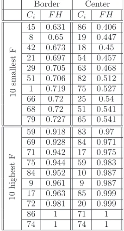
is possible to expose a study that can exhibit a specific size, shape and area(s) for a searching/detection process. For example, we examine the center area of images in DB with 16-area splitting. From Tab.8, we saw that there are five categories having frequency more than 50% : mirror, tail light (of car), hat, mailbox, head (of person). If we would like search these categories in images, we could begin the process by the center area.
1st line 2nd line 3rd line 4th line Ci FH Ci FH Ci FH Ci FH H o ri zo n ta l li n es 10 sm a ll es t F H 8 0.449 33 0.485 18 0.206 23 0.208 20 0.629 73 0.514 19 0.227 22 0.531 73 0.699 62 0.521 32 0.237 59 0.606 21 0.718 21 0.528 54 0.257 67 0.714 10 0.747 47 0.572 30 0.258 17 0.78 80 0.75 14 0.575 7 0.275 50 0.786 1 0.755 86 0.593 63 0.295 52 0.804 44 0.756 49 0.616 41 0.321 39 0.818 45 0.789 68 0.627 46 0.333 40 0.83 27 0.804 39 0.636 51 0.339 6 0.831 1 0 h ig h te st F H 71 1 77 1 44 0.967 79 0.999 66 1 72 1 83 0.97 86 1 54 1 82 1 76 0.972 74 1 51 1 71 1 42 0.978 44 1 46 1 66 1 8 0.983 80 1 23 1 54 1 14 0.986 75 1 65 1 23 1 10 0.996 38 1 64 1 17 1 20 0.999 27 1 59 1 59 1 79 0.999 8 1 52 1 52 1 80 1 10 1 V er ti ca l li n es 1 0 sm a ll es t F H 42 0.717 54 0.6 82 0.609 39 0.575 51 0.724 82 0.658 81 0.629 66 0.64 79 0.727 41 0.678 47 0.656 22 0.703 21 0.753 66 0.68 33 0.657 29 0.725 40 0.76 27 0.683 75 0.666 47 0.729 77 0.761 45 0.684 21 0.683 46 0.729 34 0.771 19 0.685 86 0.687 62 0.739 16 0.774 34 0.696 62 0.695 15 0.743 53 0.777 46 0.708 51 0.697 41 0.749 60 0.781 18 0.708 27 0.697 78 0.766 1 0 h ig h es t F H 75 0.944 9 0.994 10 0.982 17 0.951 84 0.962 69 0.999 59 0.983 56 0.955 9 0.971 85 0.999 9 0.995 69 0.964 17 0.975 20 0.999 69 0.999 9 0.966 72 0.981 71 1 85 0.999 59 0.967 59 0.983 72 1 84 0.999 75 0.972 69 0.999 74 1 80 1 14 0.972 61 1 17 1 71 1 72 0.981 86 1 59 1 74 1 71 1 74 1 52 1 17 1 74 1
Table 7 –Ranking of categories according to particular location in 16-area splitting.
4
Binary relationships
A binary relationship links two entities of distinct categories together in an image. It can be a co-occurrence or a spatial relationship. From the 86 categories of the database used, there are 3655 possible binary relationships between categories. Among them, we observed first that 879 couples of categories never occur together. For more details, the reader can consult Fig.13 which present a map of co-occurrences categories and Fig.14 for a map showing absent couples. Before studying spatial binary
Border Center Ci F H Ci F H 1 0 sm a ll es t F 45 0.631 86 0.406 8 0.65 19 0.447 42 0.673 18 0.45 21 0.697 54 0.457 29 0.705 63 0.468 51 0.706 82 0.512 1 0.719 75 0.527 66 0.72 25 0.54 68 0.72 51 0.541 79 0.727 65 0.541 1 0 h ig h es t F 59 0.918 83 0.97 69 0.928 84 0.971 71 0.942 17 0.975 75 0.944 59 0.983 84 0.952 10 0.987 9 0.961 9 0.987 17 0.963 85 0.999 72 0.981 20 0.999 86 1 71 1 74 1 74 1
Table 8 –Ranking of categories according to "border" and "center" locations in 16-area. splitting.
relationships, we examine co-occurrence relationships.
4.1 Co-occurrence relationships
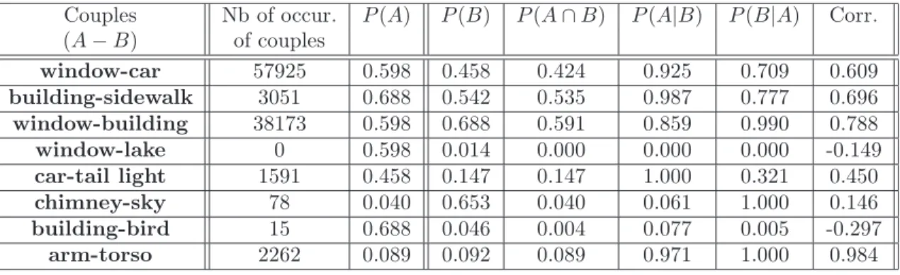
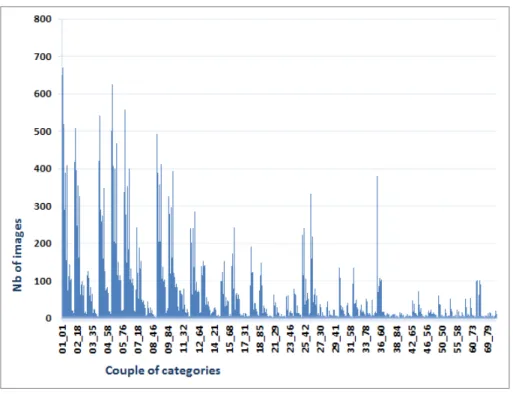
To begin, we give an example. In DB, window appears in 677 images and car in 519 images. This couple of categories appears together in 480 images. Then, we can conclude that their co-occurrence relationship is quite remarkable : for instance, 92% of the images containing a car also contain a window. This rate corresponds to a conditional probability, denoted P (window|car). Fig.15 gives an idea of the distribution of the number of images where all the category couples appear. Couples having a high number of occurrences are listed in Tab.9. Additionally, we can compute their correlation to learn more about the co-occurrence of such couples. Hence, these measures can help understanding better which category’s presence conducts to the presence or absence of another category. Statistics for some couples can be found in Tab. 9.
The correlation score resumes in one value the presence or absence together of two categories and especially the strength of this knowledge. We can apply the formula of equation 1. Variable xi shows the presence of at least on instance of category Cj in an image Ii, then xi = 1 if this condition is satisfied, otherwise xi = 0. Variable yi concerns another category Ck. Then ¯x and ¯y are their average occurrence number in database. Hence, if a couple’s correlation is negative, then this couple is rarely present in a same image. The highest score obtained is 0.984 for torso-arm ; in fact, only 3 couples have a correlation higher than 0.8 (the distribution of these correlation is displays in Fig.37 of Annex
Figure 13 – Occurrence relationships between two categories in DB.
Couples Nb of occur. P (A) P (B) P (A ∩ B) P (A|B) P (B|A) Corr. (A − B) of couples window-car 57925 0.598 0.458 0.424 0.925 0.709 0.609 building-sidewalk 3051 0.688 0.542 0.535 0.987 0.777 0.696 window-building 38173 0.598 0.688 0.591 0.859 0.990 0.788 window-lake 0 0.598 0.014 0.000 0.000 0.000 -0.149 car-tail light 1591 0.458 0.147 0.147 1.000 0.321 0.450 chimney-sky 78 0.040 0.653 0.040 0.061 1.000 0.146 building-bird 15 0.688 0.046 0.004 0.077 0.005 -0.297 arm-torso 2262 0.089 0.092 0.089 0.971 1.000 0.984
Table 9 – Couples of categories having either a highest number of occurrences or a highest conditional probability or a highest correlation.
C.1, some obvious scores can be found in Tab.18 of the same Annex). The lowest score obtained is −0.297 for couple building-bird (view Table 9). Hence, any couple in database has a strong
decor-Figure 14 – Couples of two categories that do not appear jointly in images of DB.
relation state. These results cannot conduct to the conclusion on correlation or decorrelation of most of the couples of categories.
But conditional probabilities can help to go deeper in the analysis. The conditional probability is computed as P (B | A) = P(A∩B)P(A) . P (A) and P (B) is presence probability of A and B respectively. P (A) = NI(A)
NT where NI(A) number of images where A appears and NT number of images of DB.
P (A ∩ B) is presence probability of the couple (A, B). For example, P (building|sidewalk) is very high (see Table 9). That means that, in detecting a sidewalk, we can expect finding a building in the same image. Such relationship should be integrated with benefit in a knowledge-based system dedicated to artificial vision. Indeed, sidewalks are easy to detect because of their specific and universal visual appearance, while the variability of buildings makes them harder to detect. Then the prior detection of a sidewalk would contribute to facilitate the detection of a building by reducing the number of images to process. This reasoning can be generalized to other couples of categories, since in total, there are
Figure 15 – Number of images where couples of categories appear in.
141 conditional probabilities higher than 0.95. Note that 66 of them are equal to 1 (see examples in Table 9), making the possibility of replacing the detection step of one category by the detection step of another, if easier, to find images of that category. All these measures are available on the website2 of this work. Their distribution is displays in Fig.38 of Annex C.1.
4.2 Binary spatial relationship
In last years, there have been many approaches proposed for representing binary spatial relation-ships. They can be classified as topological, directional or distance-based approaches (see [4] for more details), and can be applied on symbolic objects or low level features. Here, we have focussed on re-lationships between the entities of the database described in terms of directional rere-lationships with approach 9DSpa [7], of topological relationships [3] and of a combination of them with 2D projections [9]. We do not use orthogonal [2] and 9DLT relationship [1] because of its inconveniences mentioned in [7]. The detail of each approach is explained in the following sections.
4.2.1 9DSpa relationships
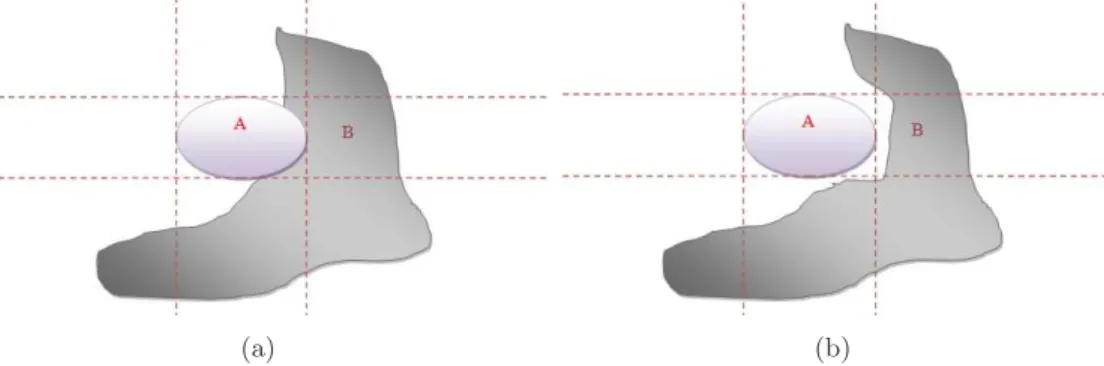
9DSpa describes directional relationships between a reference entity and another one based on the combination of 9 codes associated to areas orthogonally built around the MBR (Minimum Bounding Rectangle) of the reference entity. To complete this description, the autors take into account topolo-gical relationships. Because we want to study distinctly topolotopolo-gical relationships, we examined only
(a) (b)
Figure 16 – Original 9DSpa coding gives the same code for these two cases : 11100111 = 231.
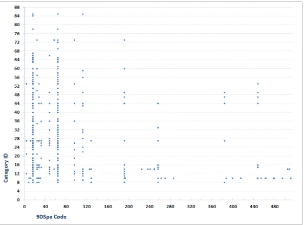
Figure 17 – Distribution of the 9DSpa codes for each category in DB.
the directional part of this approach. With the original 9DSpa approach, the description of the code uses only 8 bits, then, the center (or MBR of reference object) is coded by 0. With this type of code, we cannot identify if the second entity in a couple overlaps the MBR of reference one (see example in Figure 16). Therefore, we use a new description based on 9 bits to recognize the intersection between two entities (see Table 10).
Firstly, we present a overview of the 9DSpa codes that can be encountered for each category in Fig.17. 9DSpa approach gives 511 possible codes. But we saw that several codes are never used and
Figure 18 – Distribution of 9DSpa codes. 000000100 = 004 000000010 = 002 100000000 = 256 000001000 = 008 000000001 = 001 010000000 = 128 000010000 = 016 000100000 = 032 001000000 = 064
Table 10 –Modified codes in 9DSpa approach.
be not associated with any category. In fact, similar to 9-area splitting, with 9DSpa approach, we can build only 218 theoretically authorized codes. In DB, we have found 206 codes among these theoretical ones. In interpreting horizontally Fig.17, we see that one category Cj can be associated only to some 9DSpa codes. This information can be integrated usefully in a knowledge base dedicated to artificial vision. For example, in an image where an instance of category Cj was detected, we suppose that another category Cz can appear, and we would like localize this category. Quickly, we can give the priority only to the searching areas around Cj associated to some codes relevant with Cj. This action can reduce considerably the searching time. Interpreting vertically Fig.17, we observe that the most frequent codes are : 004 ( ), 016 ( ), 064 ( ), 256 ( ) with respectively probabilities 14%, 13%, 14%, and 13% (see distribution of 9DSpa codes in Fig.18). Furthermore, we can use the probability of each 9DSpa code for each couples of categories. Some examples about these probabilities are listed in Tab 19 of Annex C.2.
We examine now some particular examples. With category chimney, 9DSpa relationship of this reference category with others categories is resumed in Fig.19 and 40(b) of Annex C.2). In accordance
Figure 19 – Distribution of 9DSpa codes across categories by considering chimney as reference entity
(a)Chimney is reference category (b)Roof is reference category
Figure 20 – 9DSpa relationship between category chimney and category roof.
with reality, the statistics show that chimney is usually above other categories. Some other examples concerning roof, car, road also are cited in Fig.40 of Annex C.2. Moreover, we can study 9DSpa relationship between chimney and a particular category, for example with roof (see Figure 20). This couple obtains the three best probabilities of presence 0.10, 0.14 and 0.17 with respective areas , and . These results can provide an advantage in limiting a searching area for a target entity when knowing the location of reference one. During an object detection and localization task, this knowledge gives the possibility to constrain the search of the target object to priority searching areas in the image and to corresponding object’s size, given a reference object. All the associated statistics are available
on the website2 of this work.
4.2.2 Topological relationship
Code Label Code Label Code Label Code Label (0) disjoint (1) meets (2) overlaps (3) contains (4) insides (5) equals (6) covers (7) covered by
Table 11 –Codes in topological approach.
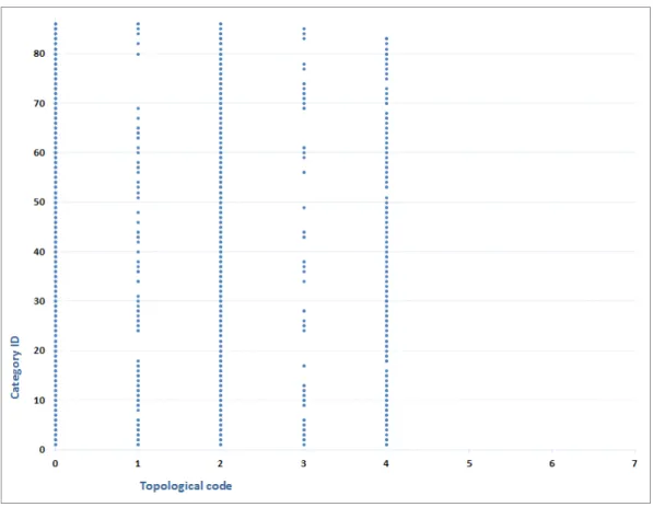
Figure 21 – Map of co-occurrence relationships between topological codes and categories in database.
The description of topological relationships provides eight types of relationships (represented in Table 11). We remark that, in DB, ”equal”, ”cover”, and ”coverby” do not appear (see Figure 22). ”Disjoint” is very frequent with a frequency more than 94%. The second position is for ”overlap” with a frequency around 2.8%. ”Contain” and ”inside” are present only 0.7% and 1.1% consecutively. "Meet" relationship is dully represented (0.3%) : its number of occurrences is small because the notion of strict adjacency between high-level objects is not common in natural contents such those of the database and because of manual annotation. Meanwhile, in literature "meet" is a popular relationship often used with some image analysis techniques such as region segmentation that generates adjacent regions by definition, with application to specific domains, e.g. satellite imagery.
Figure 22 – Frequency of topological relationships in DB.
(a)Road - Car. Road is reference category (b)Chair - Table. Table is reference category
Figure 23 – Distribution of the topological relationship between two categories for two different couples of categories.
The distribution of topological is clearly different according to couples of categories, then it can be useful in certain cases, for example in object localization. In Fig.23(a), we observed that a car appears mostly inside or overlaps regions occupied by a road. Hence, for searching a car in an given image, it is possible to begin on a region of a road if this last is already located. Meanwhile, ”disjoint” information of couple table-chair (see Fig.23(b)) could not provide any profitable information and could complicate the searching of chair based on the presence of table whose size in an image may
be usually small.
More generally, we can say that statistics on topological relationships do not provide a discrimina-tive information. With this approach, it is difficult to get a typical interpretation or conclusion for a couple of categories, except for some special categories like road and car. However, these statistical results can be used as a supplementary information for other approaches.
4.2.3 2D projection relationships
Similarly to topological approach, 2D projection approach is one of basic approach in image domain. The 2D projections approach associates 7 basic operators plus 6 symmetric ones (denoted by adding symbol "*" to the basic ones, see Tab 12) to each image axis, leading to 169 possible 2D relationships between MBR of entities.
code 1 2 3 4 5 6 7 8 9 10 11 12 13 Operator < < ∗ | |∗ / /∗ ] [ % = ]∗ [∗ %∗
Table 12 –codes in 2D projection approach [9].
In the same way as in previous sections, we can study co-occurrence between 2D operators and categories (see Figure 24 for x axis and Figure 25 for y axis), the frequency of occurrence of each 2D operator (see Figure 26(a) for x axis and Figure 26(b) for y axis). A concrete example is represented in Fig.27. We observe that 1D relationships |, |∗, ], ]∗, [, [∗ and = are not present at all on x or y axes. This result confirms that adjacency relationship is not noticeable in DB, and it also shows that 2D projections do not describe well this relationship, since they are not able to detect it here. Operators < and < ∗ are the most frequent. It confirms partially the high frequency of ”disjoint” relationship
in topological approach, and moreover, of areas with 9DSpa. In fact, operator < associated
with x axis corresponds to areas in 9DSpa. Thus, the intersection of frequencies of <
and < ∗ on axis x and y explains partially frequency of 9DSpa codes.
4.2.4 Summary of statistic
Table 13 presents a summary of the statistics obtained with DB fir the three representations of spatial relationships studied.
Approach Nb of possible Nb of effective Relationships with best relationships relationships occurrences (and frequency in %)
9DSpa 511 206 (14%), (13%), (14%), (13%)
Topological rel. 8 5 "Disjoint" (94%)
2D projections 169 36 < (37%), < ∗ (37%)(averaged on x,y axes) Table 13 –Binary spatial relationships studied and related main statistics.
Figure 24 – Map of co-occurrence relationships between 2D projection operators and categories on x axis.
Figure 25 – Map of co-occurrence relationships between 2D projection operators and categories on y axis.
Among all the possible relationships existing theoretically, only a subset was effectively found in the database for each approach. The subset is particularly small with 9DSpa and 2D projections. This result
(a) On x axis (b) On y axis
Figure 26 – Distribution of 2D projection codes on each image axis.
(a) On x axis (b) On y axis
Figure 27 – Distribution of 2D projection relationships between sea and mountain.
leads to the first conclusions that the digital codes of these relationships could be optimized and that indexing them would more benefit from data driven than space driven indexes. Moreover, among these three approaches, we think that 9DSpa is the one that allows providing the most relevant statistical knowledge for future interpretations. In particular, it is possible to deduce from them the probability of presence of a given entity in an area having a given directional relationship with a reference entity, as well as an indication on its size. During an object detection and localization task, this knowledge gives the possibility to constrain the search of the target object to priority searching areas in the image and to corresponding object’s size, given a reference object. All the associated statistics are available on the website2 of this work.
5
Ternary relationships
A ternary relationship describes a relationship of a triplet of categories. Similarly to binary rela-tionships, we examined co-occurrence and spatial relationships.
Figure 28 – Frequency of each triplet presence in DB.
Co-occurrence relationships
We continued to examine co-occurrence relationships for triplets of categories. We found 38031 present triplets in total knowing that we can have C3
86= 102340 possible triplets where order does not matter. We could compute the frequency of presence of each triplet. Fig.28 gives this frequency for each possible triplet. We observed that the most frequent triplets are (window-building-sidewalk) and (building-sidewalk-road), that have frequencies of 0.5013 and 0.4872 respectively.
Then we have calculated the correlation of each triplet by adapting the basic function (see equation 1) to relationship between a category and a couple of other categories that is present in database. For a triplet (Cj− (Ck− Cz)), if Cj is present in image Ii, then xi = 1 otherwise xi= 0. If couple (Ck− Cz) is present in image Ii, then yi= 1 otherwise yi = 0. Therefore, we examined 86 ∗ (85 ∗ 84/2) = 307020 possible combinations. We obtained highest score 0.9891 for triplet (torso -(building - arm)) and lowest score −0.2494 for triplet (water -(window-building)). Only 272 triplets have a correlation score more than 0.5. In Tab.14, we present the 40 triplets having highest or lowest correlation. We observed that there are the link between this correlation and correlation of couples of categories pre-sented in previous section 4. In fact, the highest correlation in this section concerns two categories 64 (torso) and 65(arm), that is the same result for correlation between couples.
20 triplets having highest correlation 20 triplets having lowest correlation Triplet (A- (B-C)) Corr. Triplet (A- (B-C)) Corr. ( torso - ( building - arm ) ) 0.9891 ( water - ( window - building ) ) - 0.2494 ( arm - ( building - torso ) ) 0.9786 ( sidewalk - ( sky - mountain ) ) - 0.2452 ( arm - ( person - torso ) ) 0.9786 ( mountain - ( building - sidewalk ) ) - 0.2434 ( torso - ( person - arm ) ) 0.9784 ( building - ( plant - flower ) ) - 0.2357 ( arm - ( head - torso ) ) 0.9732 ( bird - ( window - building ) ) - 0.235 ( torso - ( head - arm ) ) 0.9729 ( mountain - ( window - sidewalk ) ) - 0.2329 ( arm - ( person - head ) ) 0.9681 ( water - ( building - sidewalk ) ) - 0.2289 ( torso - ( building - head ) ) 0.962 ( water - ( building - road ) ) - 0.2285 ( arm - ( building - head ) ) 0.9572 ( flower - ( building - road ) ) - 0.2242 ( head - ( person - arm ) ) 0.9532 ( water - ( window - road ) ) - 0.2197 ( torso - ( person - head ) ) 0.9517 ( mountain - ( sidewalk - road ) ) - 0.2194 ( head - ( building - arm ) ) 0.9425 ( flower - ( building - sidewalk ) ) - 0.2144 ( head - ( torso - arm ) ) 0.9425 ( water - ( window - sidewalk ) ) - 0.2144 ( head - ( building - torso ) ) 0.9372 ( bird - ( building - sidewalk ) ) - 0.2143 ( head - ( person - torso ) ) 0.9372 ( bird - ( building - road ) ) - 0.2141 ( torso - ( window - arm ) ) 0.9217 ( bird - ( building - sky ) ) - 0.2122 ( torso - ( sidewalk - arm ) ) 0.9217 ( flower - ( window - building ) ) - 0.2119 ( arm - ( window - torso ) ) 0.9127 ( flower - ( building - sky ) ) - 0.2119 ( arm - ( sidewalk - torso ) ) 0.9127 ( water - ( sidewalk - road ) ) - 0.2093 ( torso - ( window - head ) ) 0.8989 ( flower - ( sidewalk - road ) ) - 0.2055
Table 14 –The highest and lowest correlations between triplets of categories.
by using this function P (A|B ∩ C) = PP(A∩B∩C)(B∩C) . Differently to correlation evaluation, we examined conditional probability with only triplets appearing in database. There are 38031 ∗ 3 = 114093 possible triplets where order matter. We found 11262 triplets having score 1. We can explain partially this result from the binary conditional probability results. In previous section on binary study, we obtained 66 conditional probabilities equal to 1. We know that P (A|B) = 1 when P (A ∩ B) = P (B), then we can say : A ∩ B = B (6) ⇒ B ⊂ A (7) ⇒ ∀C|B ∩ C 6= ∅ : (B ∩ C) ⊂ A (8) ⇒ A ∩ B ∩ C = B ∩ C (9) ⇒ P (A ∩ B ∩ C) = P (B ∩ C) (10) ⇒ P (A|B ∩ C) = 1 (11)
For each couple (A, B) having P (A|B) = 1, by combining it with a category C|C 6= B ∧ C 6= A, we can obtain 66 ∗ 84 = 5544 new probabilities of 1. Alternatively, we observed that, with a couple (A, B) having P (A|B) ' 1, we can have also a high probability to obtain : ∀C|B ∩ C 6= ∅ : (B ∩ C) ⊂ A. It explains why there are a high number of score 1. In this statistic, we saw also that more than 20000 triplets have a score more than 0.6. We mention related statistics in Tab.15. For more detailed results,
we would invite you to consult our website4 .
20 triplets having highest P 20 triplets having lowest P Triplet (A- (B-C)) Prob. Triplet (A- (B-C)) Prob. window- (car -wire ) 1 leaf- ( window -building ) 0.0013 window- (car -rock ) 1 hat- ( window -building ) 0.0013 window- (car -railing ) 1 lake- (building -road ) 0.0014 window- (car -grille ) 1 leaf- (building -road ) 0.0014 window- (car -lamp ) 1 hat- (building -road ) 0.0014 window- (car -light ) 1 boat- (building -sidewalk ) 0.0015 window - (car -pot ) 1 water- (building -sidewalk ) 0.0015 window- (car -pipe ) 1 leaf- (building -sidewalk ) 0.0015 window- (car -fire escape ) 1 duck- (building -sky ) 0.0015 window - (car -chair ) 1 leaf- (building -sky ) 0.0015 window- (car -mailbox ) 1 hat- (building -sky ) 0.0015 window- (car -flower ) 1 boat- ( window -road ) 0.0015 window- (car -cross walk ) 1 sea - ( window -road ) 0.0015 window- (car -cone ) 1 water- ( window -road ) 0.0015 window- (car -table ) 1 leaf- ( window -road ) 0.0015 window- (car -umbrella ) 1 hat- ( window -road ) 0.0015 window- (car -sand ) 1 boat- ( window -sidewalk ) 0.0016 window- (car -water ) 1 sea - ( window -sidewalk ) 0.0016 window- (car -attic ) 1 water- ( window -sidewalk ) 0.0016 Table 15 –The highest and lowest conditional probabilities between triplets of categories.
Ternary spatial relationships
In last years, to our knowledge, a few approaches were proposed to describe triangular relationships of three symbolic entities. We can mention TSR approach [5] and our approach ∆-TSR [6]. By applying to a set of heterogeneous symbolic entities that do not have fixed shape and size, these approaches cannot described finally triangular spatial relationships between symbolic entities since they take into account only the center of each entity as representation of it. However, to complete this study, based on the theory of ∆-TSR, we have studies the relationships between three different categories by using ∆-T SR3D. This description is invariant to translation, 2D rotation, scale, and flip. Triangular relation-ships are built on the centers of three entities. The first component of ∆-T SR3D is the identification of the triplet of categories, the second and the third components are consecutively the first and the second angles of triangle obtained from the three centers. They correspond to angles a1and a2in Fig.32.
Firstly, we present a general vision on approach’s second component in all DB with Fig. 29 and 30. We observed that this component is distributed quasi homogeneously in interval [0..180]. Then, with the ternary relationship, we can say it is complex to give a direct interpretation, for example to predict an area of searching, by using simply an angle. Although, this relationship can be useful for a representation fuzzy relationship like ”between” relationship. Suppose that we do not take into account
Figure 29 – Statistics of second component of ∆-T SR3D.
Figure 30 – Resume of statistics of second component of ∆-T SR3D.
the shape of category’s instance, the ”between” relationship can be used by restricting the value of the two angles in ∆-T SR3D. For example, a third entity C3 can be viewed "between" C1 and C2 when a1 <= 60 and a2 <= 60 (see Figure 31). If we take into account the entity’s shape, we can combine the 9DSpa approach with ∆-T SR3D to get a definition more complete of ”between” relationship. We
have computed the probability of the third category to be ”between” the two first categories in triplet (see Figure 32). We found 3376 triplets having probability score more than 0.5. For example, when we find a sidewalk and a chair in an image, if there is a motobike in this image, we could believe that this motorbike would be probably ”between” these two first entities since the corresponding probabi-lity is 0.978. In the same way, the same study for the first or second category in triple can be done easily.
Figure 31 – Illustration of relationship ”between” : Category C3 is between two other categories in ∆-T SR3D.
Figure 32 – Category triplets satisfying "between" relationship with ∆-T SR3D.
Because of limits of the spatial representation of ternary relationships for symbolic entities, we did not conduct additional statistical study on this type relationship. ∆-TSR provided more many advantages with low level feature like interest points. We think that this approach can be relevant for symbolic entities if we know how to associate other contextual information of category to it. It can
surely be done in some domains like medical domain where ∆-TSR could show its ability on homoge-neous entities having a fixed size and shape.
6
Conclusion
We have presented a statistical study on spatial relationships of categories of entities from a public database of annotated images. This study provides a cartography of the spatial relationships that can be encountered in a database of heterogeneous natural contents. We think that it could be integrated with benefit in a knowledge-based system dedicated to artificial vision and CBIR, in order to enrich the description of the visual content as well as to help to choose the most discriminant type of re-lationships for each use case. Here, we have focussed on the analysis of unary, binary, and ternary relationships. Study on unary relationships highlights trends on location of categories of entities in the image. These measures allows to determine the probability of the presence of a category in a given area, and to perform spatial reasoning. In the same way, study on binary relationships allows deducing the probability of presence of a category in an area regarding the location of another reference category. In addition, it gives indications on the relevance of the tested representations of these relationships. Ternary spatial relationships were already studied. Because of limits of the spatial representation of ternary relationships for symbolic entities, we did not conduct deeper statistical study on this type relationship.
This work was done on a manually annotated database of one thousand images. Therefore, it is evident that these statistics will have to be confirmed or refined on other image databases of larger size. However from now, we think that these measures can help us, on the one hand, to better understand which kinds of spatial relationship should be employed for a given problem and how to model them. On the other hand, such statistics can help to start a knowledge base on these relationships, that can be applied quickly to some topical problems of artificial vision and CBIR such as object detection, recognition or retrieval in a collection.
References
[1] C. Chang. Spatial match retrieval of symbolic pictures. Journal of Information Science and Engineering, 7(3) :405–422, 1991. 20
[2] S.-K. Chang and E. Jungert. A spatial knowledge structure for image information systems using symbolic projections. IJCC, 1986. 20
[3] M. J. Egenhofer and K. K. Al-Taha. Reasoning about gradual changes of topological relationships. In Proc. of the International Conference GIS, pages 196–219, London, UK, 1992. Springer-Verlag. 1, 20 [4] V. Gouet-Brunet, M. Manouvrier, and M. Rukoz. Synthèse sur les modèles de représentation des relations
spatiales dans les images symboliques. RNTI, (RNTI-E-14) :19–54, 2008. 1, 20
[5] D. Guru, P. Punitha, and P. Nagabhushan. Archival and retrieval of symbolic images : An invariant scheme based on triangular spatial relationship. Pattern Recognition Letters, 24(14) :2397–2408, 2003. 31
[6] N. V. Hoàng, V. Gouet-Brunet, M. Rukoz, and M. Manouvrier. Embedding spatial information into image content description for scene retrieval. Pattern Recognition, 43(9) :3013–3024, 2010. 31
[7] P. Huang and C. Lee. Image Database Design Based on 9D-SPA Representation for Spatial Relations. TKDE, 16(12) :1486–1496, 2004. 1, 20
[8] D. Mayhew. Principles and guidelines in software user interface design. Prentice-Hall, 1992. 11
[9] M. Nabil, J. Shepherd, and A. H. H. Ngu. 2D projection interval relationships : A symbolic representation of spatial relationships. In Symposium on Large Spatial Databases, pages 292–309, 1995. 20, 26
[10] J. Nogier. Ergonomie du logiciel et design Web. Dunod, 2005. 11
[11] J. Park, V. Govindaraju, and S. N. Srihari. Genetic engineering of hierarchical fuzzy regional representations for handwritten character recognition. International Journal on Document analysis and recognition, 2000. 8
[12] B. Russell, A. Torralba, K. Murphy, and W. Freeman. Labelme : a database and web-based tool for image annotation. In Proc. of the International Journal of Computer Vision, Volume 177(Issue 1-3) :157–173, 2008. 2
[13] W. Wang, A. Zhang, and Y. Song. Identification of objects from image regions. Int. Conf. on Multimedia and Expo, 2003. 8
A
Annotated image database
A.1 Statistics on categories
Categ. ID Corr. Categ. ID Corr. Categ. ID Corr. Categ. ID Corr.
01 0.776 23 0.230 45 0.093 67 0.11 02 0.664 24 0.225 46 0.044 68 0.131 03 0.248 25 0.495 47 0.211 69 0.117 04 0.652 26 0.568 48 0.178 70 0.145 05 0.637 27 0.231 49 0.319 71 0.030 06 0.548 28 0.238 50 0.131 72 0.077 07 0.303 29 0.191 51 0.231 73 0.136 08 0.169 30 0.351 52 0.121 74 0.000 09 0.107 31 0.232 53 0.287 75 0.102 10 0.057 32 0.371 54 0.134 76 0.137 11 0.253 33 0.220 55 0.217 77 0.106 12 0.528 34 0.247 56 0.115 78 0.126 13 0.400 35 0.234 57 0.181 79 0.109 14 0.192 36 0.641 58 0.299 80 0.125 15 0.379 37 0.147 59 0.124 81 0.107 16 0.405 38 0.144 60 0.299 82 0.059 17 0.121 39 0.118 61 0.091 83 0.163 18 0.316 40 0.186 62 0.044 84 0.207 19 0.343 41 0.103 63 0.304 85 0.122 20 0.098 42 0.133 64 0.295 86 0.029 21 0.242 43 0.266 65 0.304 22 0.141 44 0.315 66 0.118
B
Unary relationships
B.1 Results analysis
We were interested how to define the function allowing to determinate the theoretically authorized codes from a set of initial ones (the smallest atomic ones). Suppose that an image I is splitted in n atomic areas As. The code representing Asis noted cod(As). The set of areas that are joint by edge with Asis noted edge(As). For two atomic areas Asi and Asj, we call comb(Asi, Asj) the function combining these two areas to give a new complex area. comb(Asi, Asj) = null if Asj ∈ edge(A/ si) Ak|Ak= Asi∪ Asj otherwise (12) with :
cod(Ak) = cod(Asi) + cod(Asj) (13)
edge(Ak) = edge(Asi) ∪ edge(Asj) \ {Asi, Asj} (14)
Now, we can define the function F C allowing to indicate all theoretically authorized areas from a set of two atomic areas.
F C({Asi, Asj}) = {Asi, Asj, comb(Asi, Asj)} (15)
Suppose that we have a set Ai a complex area containing more than two atomic areas, then, we can define recursively the function F C on Ai :
F C(Ai) = F C({Asi, Ft(Ai {Asi})}) (16) = {F C({Asi, Ak|Ak∈ F C(Ai {Asi})})} (17)
See examples of F C(Ai) in Tab.17 for building vertical/horizontal line, border or center area with each type of splitting.
Ai F (Ai) 9-area codes {1, 8, 9} {1, 8, 64, 9, 72, 73} {2, 16, 128} {2, 16, 128, 18, 144, 146} {4, 32, 256} {4, 32, 256, 36, 288, 292} {1, 2, 4} {1, 2, 4, 3, 6, 7} {8, 16, 32} {8, 16, 32, 24, 48, 56} {64, 128, 256} {64, 128, 256, 192, 384, 448} 16-area codes {1, 16, 256, 4096} {1, 16, 256, 4096, 17, 272, 4352, 273, 4368, 4369} {2, 32, 512, 8192} {2, 32, 512, 8192, 34, 544, 8704, 546, 8736, 8738} {4, 64, 1024, 16384} {4, 64, 1024, 16384, 68, 1088, 17408, 1092, 17472, 17476} {8, 128, 2048, 32768} {8, 128, 2048, 32768, 136, 2176, 34816, 2184, 34944, 34952} {1, 2, 4, 8} {1, 2, 4, 8, 3, 6, 12, 7, 14, 15} {16, 32, 64, 128} {16, 32, 64, 128, 48, 96, 192, 112, 224, 240} {256, 512, 1024, 2048} {256, 512, 1024, 2048, 768, 1536, 3072, 1792, 3584, 3840} {4096, 8192, 16384, 32768} {4096, 8192, 16384, 32768, 12288, 24576, 49152, 28672, 57344, 61440} {32, 64, 112, 224, 512, 1024} {32, 64, 96, 512, 544, 608, 1024, 1088, 1120, 1536, 1632}
The border area { 1, 2, 3, 4, 6, 7, 8, 12, 14, 15, 16, 17, 19, 23, 31, 128, 136, 140, 142, 143, 159, 256, 272, 273, 275, 279, 287, 415, 2048, 2176, 2184, 2188, 2190, 2191, 2207, 2463, 4096, 4352, 4368, 4369, 4371, 4375, 4383, 4511, 6559, 8192, 12288, 12544, 12560, 12561, 12563, 12567, 12575, 12703, 14751, 16384, 24576, 28672, 28928, 28944, 28945, 28947, 28951, 28959, 29087, 31135, 32768, 34816, 34944, 34952, 34956, 34958, 34959, 34975, 35231, 39327, 47519, 49152, 51200, 51328, 51336, 51340, 51342, 51343, 51359, 51615, 55711, 57344, 59392, 59520, 59528, 59532, 59534, 59535, 59551, 59807, 61440, 61696, 61712, 61713, 61715, 61719, 61727, 61855, 63488, 63616, 63624, 63628, 63630, 63631, 63647, 63744, 63760, 63761, 63763, 63767, 63775, 63872, 63880, 63884, 63886, 63887, 63888, 63889, 63891, 63895, 63896, 63897, 63899, 63900, 63901, 63902, 63903} Table 17 –Sets of codes presenting a location on horizontal/vertical line in image.
C
Binary relationships
C.1 Co-occurrence relationships Cat.ID 01 02 05 06 10 13 16 20 28 34 43 74 85 01 0.776 02 0.609 0.664 05 0.788 0.566 0.637 06 0.733 0.613 0.696 0.548 10 0.275 0.2 0.35 0.209 0.057 13 0.124 0.13 0.059 0.111 -0.024 0.4 16 0.363 0.371 0.376 0.371 0.245 0.066 0.405 20 0.043 0.071 0.026 0.036 0.071 0.072 -0.005 0.098 28 0.191 0.132 0.174 0.167 0.12 0.117 0.083 0.047 0.238 34 0.154 0.104 0.153 0.128 0.113 0.049 0.151 0.087 0.248 0.247 43 -0.13 -0.066 -0.035 -0.132 0.072 0.039 0.053 -0.041 0.003 0.009 0.266 74 -0.149 -0.097 -0.117 -0.133 0.007 -0.063 -0.045 -0.012 -0.032 -0.031 0.163 0 85 -0.071 -0.033 -0.008 -0.112 0.092 -0.069 -0.052 -0.013 -0.005 -0.033 -0.013 -0.015 0.122Table 18 – Correlation scores of some couples of categories in DB. The scores on the diagonal represent the inter-class correlation.
Figure 33 – Distribution of categories according to code 16 in 9-area splitting.
Figure 34 – Distribution of categories according to code 128 in 9-area splitting. Cat. ID 01 Cat. ID 02 9Dspa code Number of occ.
01 02 16 21774 02 01 256 21774 01 02 64 19349 02 01 4 19349 01 36 64 18852 36 01 4 18852 01 36 16 17934 36 01 256 17934 01 26 64 16626 26 01 4 16626 01 26 16 16337 26 01 256 16337 05 01 1 13334 01 05 511 11702 09 01 2 11640 01 09 112 11598 06 01 2 8222 01 06 112 8176 01 12 16 7084 12 01 256 7084
Figure 38 – Distribution of conditional probabilities for every category pairs in DB.
(a)Roof is reference category (b)Chimney is reference category
(c)Car is reference category (d)Road is reference category
Figure 40 – Examples of statistical study on 9DSpa relationships between a reference category and others.