Assorted results in boolean function complexity, uniform sampling and clique partitions of graphs

(1)

Assorted results in boolean function complexity,

uniform sampling and clique partitions of graphs

by

Jake Wellens

Submitted to the Department of Mathematics

in partial fulfillment of the requirements for the degree of

Doctor of Philosophy in Mathematics

at the

MASSACHUSETTS INSTITUTE OF TECHNOLOGY

June 2020

c

○ Massachusetts Institute of Technology 2020. All rights reserved.

Author . . . .

Department of Mathematics

May 1, 2020

Certified by . . . .

Henry Cohn

Senior Principal Researcher at Microsoft Research New England and

Adjunct Professor of Mathematics at MIT

Thesis Supervisor

Accepted by . . . .

Jon A. Kelner

Chairman, Department Committee on Graduate Theses

(2)

(3)

Assorted results in boolean function complexity, uniform

sampling and clique partitions of graphs

by

Jake Wellens

Submitted to the Department of Mathematics on May 1, 2020, in partial fulfillment of the

requirements for the degree of Doctor of Philosophy in Mathematics

Abstract

This thesis consists of three disparate parts. In the first, we generalize and extend recent ideas of Chiarelli, Hatami and Saks to obtain new bounds on the number of relevant variables for a boolean function in terms of its degree, its sensitivity, and its certificate and decision tree complexities, and we also sharpen the best-known polynomial relationships between some of these complexity measures by a constant factor. In the second part, we show that the Partial Rejection Sampling method of Guo, Jerrum and Liu can solve a handful of natural sampling problems that fall outside the guarantees of the authors’ original analysis. Finally, we revise and make partial progress on a conjecture of De Caen, Erdős, Pullman and Wormald on clique partitions of a graph and its complement, building on ideas of Keevash and Sudakov.

Thesis Supervisor: Henry Cohn

Title: Senior Principal Researcher at Microsoft Research New England and Adjunct Professor of Mathematics at MIT

(4)

(5)

Acknowledgments

I owe a great deal of thanks to my thesis advisor, Henry Cohn, who was always ready and willing to discuss any mathematical thought, so long as I was ready and willing to make the trek from Building 2 to Microsoft. He allowed me the freedom to pick up any problem that sparked my interest, and was never short on suggestions for where to look next when I was ready to move on. In particular, he introduced me to partial rejection sampling, which led to the work in Chapter 3 of this thesis.

I’d also like to thank the other members of my thesis committee – Elchanan Mossel and Jon Kelner. Although they were some of the busiest people in the department, both Elchanan and Jon were always generous with their time, their mathematical wisdom and their encouragement.

To my officemates, Fred Koehler and John Urschel: thanks for enduring my boxes, my phone interviews, my “wall art” and my fidget spinner phase. Special thanks to John for convincing me to abandon PDEs in my first year and take Advanced Algorithms instead.

To my friends on the second floor, Vishesh Jain and Thao Do: thanks for all the math gossip and life advice, and for getting me to the gym. Without you two, my procrastination wouldn’t have been half as productive and lively as it was.

To my friends who followed me to Cambridge from Pasadena, Jake Marcinek and Kevin Li: thanks for being, unfailingly, about that life.

To my most inspiring teachers, Peter Kaczmar and Chris Marx: thanks for teach-ing me how to see the forest and the trees simultaneously.

To my sister Kaitlin: thanks for always being the first mover and a role model. To my mother Rose: thanks for your unwavering support, patience, honesty, hu-mor and love. They don’t make ‘em like you anyhu-more.

(6)

(7)

Chapter 1 Introduction

Each of the three chapters of this thesis is, in terms of its mathematical content, almost entirely unrelated to the others – distant cousins at best. They are alike, however, in that they are comprised of refinements, generalizations and applications of clever mathematical ideas developed by other groups of people before me. We give a very brief overview of these ideas and what we do with them below – a more satisfactory introduction can be found at the beginning of each chapter.

Let us say a boolean function 𝑓 : {0, 1}𝑛 _{→ {0, 1} is non-degenerate if it cannot} be written as a function on {0, 1}𝑛′ _{for 𝑛}′ _{< 𝑛. In 1992, Nisan and Szegedy [}₅₈_]

proved a lower bound on the degree of such functions as real multilinear polynomials. More specifically, if 𝑓 : {0, 1}𝑛 _{→ {0, 1} is a non-degenerate function of degree 𝑑,} then 𝑛 ≤ 𝑑 · 2𝑑−1_{. A recent paper of Chiarelli, Hatami and Saks [}₁₃_{] improved this} bound to 𝑛 ≤ 6.416 · 2𝑑_{, which is tight up to a constant factor. Their main idea was to} consider the potential function ∑︀

𝑖∈[𝑛]2− deg(𝐷𝑖𝑓 ) instead of the quantity ∑︀

𝑖∈[𝑛]Inf𝑖[𝑓 ], as in Nisan and Szegedy’s original proof. In Chapter 2, we introduce similar potentials based on sensitivity and certificate complexity, as well as mixtures of these measures, obtaining new results of a similar flavor. Along the way, we sharpen their result by a constant, as well as many other best-known polynomial relationships between these measures.

In Chapter 3, we explore some applications of a recent paper by Guo, Jerrum and Liu [32], in which the authors introduced a general algorithmic framework called

(10)

Par-tial Rejection Sampling for generating samples from product distributions conditional on a set of constraints being satisfied. It is shown in [32] that the procedure termi-nates with a uniform sample in an expected number of rounds which is logarithmic in the problem size, as long as (i) a Lovasz Local Lemma-like condition holds, and (ii) whenever two constraints overlap at all (in terms of the variables they depend on), they overlap significantly (loosely speaking). We apply their method to two sampling problems which do not satisfy the second condition, and yet we prove a logarithmic runtime bound for these problems.

Finally, in Chapter 4, we prove new bounds on the quantity

max 𝐺∈𝒢𝑛

cp(𝐺) + cp(𝐺),

where 𝒢𝑛is the set of all graphs on 𝑛 vertices, and cp(𝐺) is the clique partition number of 𝐺, which is defined as the minimal number 𝑟 such that there exist 𝑟 edge-disjoint cliques whose union is exactly 𝐺. (In particular, cp(𝐺) ≤ |𝐸(𝐺)|, since 𝐸(𝐺) is an edge-disjoint family of 2-cliques whose union is 𝐺.) In a 1986 paper of De Caen, Erdős, Pullman and Wormald [18], the authors show that

(︂ ₇ 25+ 𝑜(1) )︂ 𝑛2 ≤ max 𝐺∈𝒢𝑛 cp(𝐺) + cp(𝐺) ≤ (︂₁₃ 30+ 𝑜(1) )︂ 𝑛2

and conjecture that the constant ₂₅7 is optimal. We show that this is not true, by exhibiting an infinite family of graphs with cp(𝐺) = cp(𝐺) = 1₂(︁₂₅7 + ₂₀₅₀1 + 𝑜(1))︁𝑛2. We also make use of a method of Keevash and Sudakov to improve the upper bound, showing that

lim 𝑛→∞

max𝐺∈𝒢𝑛cp(𝐺) + cp(𝐺)

𝑛2 ∈ (0.28048, 0.3186).

(The content in Chapter 4 overlaps with a forthcoming joint work by the author, John Urschel and Dhruv Rohatgi [69]).

(11)

Chapter 2 On Some Extremal Properties of

Boolean Functions

2.1 Introduction

In this chapter, we investigate several fundamental questions about boolean functions

𝑓 : {0, 1}𝑛 → {0, 1}. Such functions are natural objects of study in many areas of computer science and mathematics, and therefore a fairly rich theory has developed around them in the past half century. Many important breakthroughs in active areas such as circuit complexity, PCPs and hardness of approximation, learning theory, cryptography and pseudorandomness – to name a few – are built upon an under-standing of the combinatorial and analytic properties of boolean functions. For a proper introduction to the analysis of boolean functions and their role in theoretical computer science, we refer the reader to Ryan O’Donnell’s excellent book ([61]).

Here, we concern ourselves not with these exciting applications, but rather with a few basic extremal questions about boolean functions. In particular, we focus on questions of the form, “if a boolean function 𝑓 is small in measure A, then how large can it be in measure B?”, for a variety of complexity measures A and B. In most of our results, the measure B is simply the number of relevant variables1 _of

1_{We say a variable 𝑖 ∈ [𝑛] is relevant for 𝑓 if flipping the 𝑖th bit can actually change the value of}

(12)

a function 𝑓 , while the measure A belongs to a class of well-studied, polynomially related complexity measures, including 𝑠(𝑓 ), bs(𝑓 ), deg(𝑓 ), 𝐶(𝑓 ), DT(𝑓 ), or

sensitiv-ity, block sensitivsensitiv-ity, degree, certificate complexity and decision tree/query complexsensitiv-ity,

respectively2_{. These measures arise naturally when studying various simple models} of computation. For example, the decision tree depth DT(𝑓 ) measures the worst case number of bits of 𝑥 made by the best adaptive query algorithm for computing 𝑓 (𝑥). Perhaps a more interesting model is a CREW-PRAM (Concurrent Read Exclusive Write Parallel Random Access Machine), which has been studied by computer sci-entists since at least the early 1980’s (see e.g. [10], [16], [68]). A CREW-PRAM for computing some function 𝑓 : {0, 1}𝑛 _{→ {0, 1} consists of a collection of} proces-sors, computing synchronously in parallel, communicating via a global random access memory. Beginning with a string 𝑥1, . . . , 𝑥𝑛stored in global memory cells 𝐶1, . . . , 𝐶𝑛, the computation must finish with 𝑓 (𝑥1, . . . , 𝑥𝑛) written on cell 𝐶1. At each step of

computation, each processor can read any global memory cell, do some (arbitrary) private computing and then write to a global memory cell, with the restriction that at most one processor be allowed to write to a particular global memory cell in a single step (hence the “exclusive write”). In [16] and [68], Cook, Dwork and Reischuk show that any CREW-PRAM computing a function 𝑓 requires at least Ω(log 𝑠(𝑓 )) steps in the worst case. Nisan [60] then introduced block sensitivity as a generalization of sensitivity to obtain a corresponding upper bound of 𝑂(log bs(𝑓 )) on CREW-PRAM complexity – hence tightness of the Cook-Dwork-Reischuk lower bound on CREW-PRAM complexity is equivalent to the statement bs(𝑓 ) ≤ 𝑠(𝑓 )𝐶_{, for some constant}

𝐶 < ∞. Nisan, Szegedy and others ([58], [28], [11], e.g.) conjectured this to be true (eventually with 𝐶 = 2). The so-called sensitivity conjecture remained open for some 25 years, until Hao Huang’s recent proof ([40]) of bs(𝑓 ) ≤ 𝑠(𝑓 )4_.

In light of the Cook-Dwork-Reischuk lower bound, a generic lower bound 𝑠(𝑓 ) ≥

𝑠(𝒞), for all 𝑓 in some function class 𝒞, implies that all 𝑓 ∈ 𝒞 have CREW-PRAM

complexity Ω(log 𝑠(𝒞)). The same is of course true for deg(𝑓 ) or any of the other

𝑥 and 𝑥′ in {0, 1}𝑛 such that 𝑥 and 𝑥′ differ only in the 𝑖th coordinate and 𝑓 (𝑥) ̸= 𝑓 (𝑥′).

2_{We give formal definitions of all of these quantities in section}_{2.2, but for a more comprehensive}

(13)

measures discussed above. The broadest possible class 𝒞 of boolean functions for which it is possible to obtain nontrivial lower bounds is the set of all functions with 𝑛 relevant variables, which we denote by 𝒞𝑛. The following two foundational results in this direction, concerning 𝑠(𝒞𝑛) and deg(𝒞𝑛), are due to H.U. Simon [72] and Nisan and Szegedy [58], respectively.

Theorem: (Simon, 1983) For any 𝑓 ∈ 𝒞𝑛, with 𝑠(𝑓 ) = 𝑠,

𝑛 ≤ 𝑠

2 · 4

𝑠_. _(2.1)

Theorem: (Nisan-Szegedy, 1994) For any 𝑓 ∈ 𝒞𝑛, with deg(𝑓 ) = 𝑑,

𝑛 ≤ 𝑑 · 2𝑑−1. (2.2)

Both theorems yield a Ω(log log 𝑛) lower bound on the CREW-PRAM complexity of

𝑓 ∈ 𝒞𝑛. This lower bound is tight, as witnessed by the address function

𝑓 (𝑥1, . . . , 𝑥𝑘, {𝑦𝑧}𝑧∈{0,1}𝑘) = 𝑦_(𝑥1_,...,𝑥 𝑘)

which has 𝑛 = 2𝑘 + 𝑘 relevant variables and 𝑠(𝑓 ) = deg(𝑓 ) = 𝑘 + 1 = log 𝑛 +

𝑂(log log 𝑛). In fact, Wegener [75] gave an even tighter example of a monotone function 𝑔 on 𝑛 = Ω(√1

𝑠(𝑔) · 4

𝑠(𝑔)_{) = Ω(}_√ 1 deg(𝑔)· 2

deg(𝑔)_{) relevant variables. Hence, the}

logarithmic (in 𝑛) lower bounds obtained on 𝑠(𝑓 ) and deg(𝑓 ) from (2.1) and (2.2) are tight up to a 1 + 𝑜(1) factor. However, viewed as upper bounds on 𝑛, (2.1) and (2.2) are not known to be asymptotically tight. In fact, Nisan and Szegedy’s result was recently improved, for the first time, in [13]:

Theorem: (Chiarelli, Hatami, Saks 2019) For any 𝑓 ∈ 𝒞𝑛, with 𝑑 := deg(𝑓 ),

𝑛 ≤ 6.614 · 2𝑑. (2.3)

The authors of [13] also construct an infinite family of functions of degree 𝑑 with

(14)

variables in terms of degree is 𝑛 ∼ 𝐶deg· 2𝑑, for some 𝐶deg ∈ [1.5, 6.614]. Computing

the precise value of 𝐶deg remains an open problem, one which we believe is inherently

interesting, even though such improvements are inconsequential from the perspective of PRAM lower bounds.

Unlike the Nisan-Szegedy theorem, Simon’s theorem has not been improved (as far as we are aware), nor have any tight examples been discovered. In particular, it does not appear to be known whether the extra factor of 𝑠 can be removed from (2.1), which seems like a natural question to ask in light of the recent improvement to (2.2).

Similarly, many of the known polynomial relationships between the measures

𝑠(𝑓 ), bs(𝑓 ), deg(𝑓 ), 𝐶(𝑓 ) and DT(𝑓 ) have not been improved since the initial flurries

of work in the 1990s and early 2000s. (The obvious exception being Huang’s recent proof that 𝑠(𝑓 ) even belongs in this polynomial family!) There has, however, been more recent progress in constructing separations between these measures. For exam-ple, a classical result of Nisan [60] says that 𝐶(𝑓 ) ≤ bs(𝑓 )2_{, and yet for many years}

the biggest gap exhibited by a known family of functions was 𝐶(𝑓 ) = bs(𝑓 )log4.55,

until Gilmer, Saks and Srinivasan [27] showed in 2013 that 2 is the best possible exponent in this bound. One outstanding question in this area is that of bs(𝑓 ) versus deg(𝑓 ). Nisan and Szegedy showed in [58] that

bs(𝑓 ) ≤ 2 deg(𝑓 )2, (2.4)

and other than a constant-factor improvement to bs(𝑓 ) ≤ deg(𝑓 )2 _{by Tal [}₇₃_{], neither}

this upper bound nor the bs(𝑓 ) = deg(𝑓 )log36 separation [59] has been improved in 25

years. The proof is completely analytic and makes use of V. A. Markov’s inequality for polynomials on R, while most of the best-known relationships between other com-plexity measures either have completely combinatorial/algorithmic proofs, or result from chaining together an algorithm with the bound bs(𝑓 ) ≤ deg(𝑓 )2_{. (Again, the}

notable exception is Huang’s deg(𝑓 ) ≤ 𝑠(𝑓 )2_{, which is proved using spectral graph}

(15)

best-known bound on DT(𝑓 ) in terms of deg(𝑓 ), follows from an algorithm described in [55] which computes 𝑓 using at most bs(𝑓 )·deg(𝑓 ) queries, giving DT(𝑓 ) ≤ deg(𝑓 )3

when combined with (2.4). Any progress on the bs(𝑓 ) vs. deg(𝑓 ) question is therefore interesting, in the author’s opinion.

2.1.1 New Results

In this chapter, we make modest progress on the aforementioned problems. Our main results are summarized in the following theorem:

Main Theorem: Let 𝑓 : {0, 1}𝑛 _{→ {0, 1} be such that every 𝑖 ∈ [𝑛] is relevant for}

𝑓 , and set 𝑠 := 𝑠(𝑓 ), 𝑑 := deg(𝑓 ), 𝑏 := bs(𝑓 ), 𝐶 := 𝐶(𝑓 ), and 𝐷 := DT(𝑓 ). Then

𝑛 ≤ min

{︂

4.394 · 2𝑑, 1

24

𝐶_{, 8.277 · 2}𝑑₂+𝑠_{, (log 𝑠 + 0.29) · 2}𝐶+𝑠}︂_. _(2.5)

Moreover, for each 𝑘, the number of coordinates 𝑖 ∈ [𝑛] which are not sensitive for any input 𝑥 with 𝑠𝑥(𝑓 ) ≥ 𝑘 is at most 𝑘2+𝑜𝑘(1)4𝑘. If 𝑓 is monotone, then

𝑛 ≤ min {︂ 1.325 · 2𝑑, 1 2 · 4 𝑠 , 1 4· 2 𝐷 + 2 }︂ . (2.6)

In any case, for 𝛾 :=√︁2/3 = 0.81649 . . . , we also have

𝑏 ≤ (𝛾 + 𝑜(1)) · 𝑑2 (2.7)

𝑏 ≤ (𝛾 + 𝑜(1)) · 𝑠4 (2.8)

(16)

2.2 Preliminaries

Throughout the entire chapter, 𝑓 will be a boolean function on {0, 1}𝑛_{. We will refer} to the input variables to such functions either by 𝑥𝑖 or simply by the index 𝑖, for each

𝑖 ∈ {1, . . . , 𝑛} =: [𝑛]. We define 𝑅(𝑓 ) to be the set of relevant variables (sometimes relevant coordinates) for 𝑓 , namely those 𝑖 ∈ [𝑛] for which there exists a pair of inputs

(𝑥, 𝑥′) such that 𝑥𝑗 = 𝑥′𝑗 for all 𝑗 ̸= 𝑖 and 𝑓 (𝑥) ̸= 𝑓 (𝑥

′_{). Let 𝛿}

𝑖(𝑓 ) be the indicator of whether 𝑖 is relevant for 𝑓 . We also define 𝑛(𝑓 ) = |𝑅(𝑓 )| = ∑︀

𝑖∈[𝑛]𝛿𝑖(𝑓 ) to be the number of relevant variables for 𝑓 . We say a function 𝑓 on {0, 1}𝑛 _{is non-degenerate} if 𝑛(𝑓 ) = 𝑛, that is, every variable is relevant for 𝑓 .

Sometimes it will be convenient to consider functions 𝑔 : {±1}𝑛 _{→ {±1} instead of}

𝑓 : {0, 1}𝑛 _{→ {0, 1}. Such sets of functions are clearly in bijection with one another,} e.g. via the algebraic transformations

𝑓 (𝑥1, . . . , 𝑥𝑛) ↦→ 𝑔(𝑥) := 1 − 𝑓 (1−𝑥1 2 , . . . , 1−𝑥𝑛 2 ) 2 : {±1} 𝑛 _{→ {±1}} _(2.10) 𝑔(𝑥1, . . . , 𝑥𝑛) ↦→ 𝑓 (𝑥) := 1 − 2𝑔(1 − 2𝑥1, . . . , 1 − 2𝑥𝑛) : {0, 1}𝑛→ {0, 1}(2.11)

Functions on {±1}𝑛can be expressed as a linear combination of characters 𝜒𝑆 for 𝑆 ⊆ [𝑛], where 𝜒𝑆(𝑥) =∏︀𝑖∈𝑆𝑥𝑖. These characters form an orthonormal basis with respect to the inner product ⟨𝑓, 𝑔⟩ := ₂1𝑛

∑︀

𝑥∈{±1}𝑛𝑓 (𝑥)𝑔(𝑥) = E[𝑓 (𝑥)𝑔(𝑥)], and hence any 𝑓 :

{±1}𝑛_{→ R has a unique (Fourier) expansion of the form 𝑓(𝑥) =}∑︀

𝑆⊆[𝑛]𝑓 (𝑆)^ ∏︀

𝑖∈𝑆𝑥𝑖. (The coefficients ^𝑓 (𝑆) are called the Fourier coefficients of 𝑓 .) For each coordinate 𝑖,

we define the 𝑖th directional derivative 𝐷𝑖𝑓 via 𝐷𝑖𝑓 (𝑥) = 𝑥𝑖𝑓 (𝑥)−𝑓 (𝑥

𝑖₎

2 , from which it

follows that 𝐷𝑖𝑓 (𝑥) =∑︀𝑆∋𝑖𝑓 (𝑆)𝜒^ 𝑆∖{𝑖}(𝑥). The 𝑖th coordinate influence of a function

𝑓 , denoted Inf𝑖[𝑓 ], is defined to be

Inf𝑖[𝑓 ] := Pr

𝑥∼{±1}𝑛[𝑓 (𝑥) ̸= 𝑓 (𝑥

𝑖 )]

and the total influence of 𝑓 , denoted by I[𝑓 ], is defined to be ∑︀𝑛

𝑖=1Inf𝑖[𝑓 ]. Since

(17)

the well-known Fourier formulas for influence: Inf𝑖[𝑓 ] = ∑︁ 𝑆∋𝑖 ^ 𝑓 (𝑆)2, I[𝑓 ] = ∑︁ 𝑆⊆[𝑛] |𝑆| ^𝑓 (𝑆)2

If 𝑓 is monotone, then Inf𝑖[𝑓 ] = ^𝑓 ({𝑖}) and so I[𝑓 ] = ∑︀𝑛𝑖=1𝑓 ({𝑖}). The following^ useful fact can be observed directly from the definition of influence:

Fact 2.2.1. For any 𝑖 ∈ [𝑛], and any set 𝐻 ⊂ [𝑛] with 𝑖 ̸∈ 𝐻,

Inf𝑖[𝑓 ] = E𝛼∼{0,1}𝐻[Inf_𝑖[𝑓_𝛼]].

The Fourier expansion of a function 𝑓 is the unique polynomial expansion of

𝑓 in {±1}-valued variables, and there is a corresponding (unique) polynomial for 𝑓 over {0, 1}, which we call the multilinear polynomial expansion of 𝑓 . These two

polynomials have the same degree, which we simply call the degree of 𝑓 , denoted deg(𝑓 ). From the Fourier formulas it is clear that I[𝑓 ] ≤ deg(𝑓 ). The following facts are well-known and easy to show by induction (see, e.g. [35] and [61]):

Fact 2.2.2. Let 𝑓 be a boolean function and let ∑︀ 𝑆⊆[𝑛]𝑐𝑆

∏︀

𝑖∈𝑆𝑥𝑖 be its multilinear

polynomial expansion over {0, 1}. Then for all 𝑆 ⊆ [𝑛]: 1. 𝑐𝑆 ∈ Z, and ^𝑓 (𝑆) ∈ ₂deg(𝑓 )1 · Z 2. 𝑐𝑆 = (−2)|𝑆|∑︀𝐵:𝑆⊆𝐵⊆[𝑛]𝑓 (𝐵)^ 3. ^𝑓 (𝑆) =∑︀ 𝐵⊆[𝑛],𝐵′_⊆𝑆𝑐_𝐵(−1)|𝐵 ′_| (1₂)−|𝐵∖𝐵′|

We next define a variety of complexity measures we will encounter in this chapter. As mentioned at the start of the chapter, these concepts were originally introduced because of their close relationships with various models of computation. For any string 𝑥 ∈ {0, 1}𝑛 _{and a subset 𝑆 ⊆ [𝑛], we let 𝑥}𝑆 _{denote the string obtained by} flipping the bits of 𝑥 belonging to 𝑆 and leaving the rest alone. If 𝑆 = {𝑖}, we simply write 𝑥𝑖_{to denote 𝑥 with the 𝑖th bit flipped. If 𝑓 (𝑥) ̸= 𝑓 (𝑥}𝑖_{), we say that 𝑓 is sensitive} to 𝑖 at 𝑥. The sensitivity of 𝑓 at an input 𝑥, denoted 𝑠𝑥(𝑓 ), is the number of 𝑖 ∈ [𝑛]

(18)

for which 𝑓 is sensitive to 𝑖 at 𝑥. The maximum of 𝑠𝑥(𝑓 ) over all 𝑥 ∈ {0, 1}𝑛 is called the sensitivity of 𝑓 (also maximum sensitivity of 𝑓 ), and is denoted 𝑠(𝑓 ). The

1-sensitivity (resp. 0-sensitivity) of 𝑓 , denoted 𝑠1(𝑓 ) (resp. 𝑠0_{(𝑓 )), is the maximum}

of 𝑠𝑥(𝑓 ) over all inputs 𝑥 with 𝑓 (𝑥) = 1 (resp. 0). Note that I[𝑓 ] = E𝑥[𝑠𝑥(𝑓 )] ≤ 𝑠(𝑓 ). The block sensitivity at the point 𝑥 of a boolean function 𝑓 : {0, 1}𝑛 → {0, 1}, denoted bs𝑥(𝑓 ), is the maximum number 𝑘 such that there exist 𝑘 disjoint sets

𝐵1, . . . , 𝐵𝑘 ⊆ [𝑛] (called blocks) with the property that

𝑓 (𝑥) = 𝑓 (𝑥𝐵𝑖_{), for 𝑖 = 1, . . . , 𝑘.}

We then define the block sensitivity of 𝑓 to be the maximum value of bs𝑥(𝑓 ) over all

𝑥 ∈ {0, 1}𝑛_{, and we denote it by bs(𝑓 ). If we restrict the blocks to be of size at most}

ℓ, the corresponding quantity is denoted bsℓ(𝑓 ). Clearly bs(𝑓 ) ≥ bs1(𝑓 ) = 𝑠(𝑓 ).

The certificate complexity at the point 𝑥 of a boolean function 𝑓 , denoted 𝐶𝑥(𝑓 ), is the size of the smallest set 𝑆 ⊆ [𝑛] with the property that 𝑓 is constant on the subcube of points which agree with 𝑥 on 𝑆, i.e. {𝑦 : 𝑦𝑖 = 𝑥𝑖 for all 𝑖 ∈ 𝑆}. The

certificate complexity of 𝑓 , denoted 𝐶(𝑓 ), is then defined as the maximum value of 𝐶𝑥(𝑓 ) over all 𝑥 ∈ {0, 1}𝑛. Also, let 𝐶min(𝑓 ) := min𝑥∈{0,1}𝑛𝐶_𝑥(𝑓 ). By analogy with

𝑠0_{(𝑓 ) and 𝑠}1_{(𝑓 ), we can also define 𝐶}0_{(𝑓 ), 𝐶}1_{(𝑓 ), 𝐶}0

min(𝑓 ) and 𝐶min1 (𝑓 ) in the obvious

way.

The query complexity or (deterministic) decision tree complexity of 𝑓 , denoted DT(𝑓 ), is defined to be the minimum cost of any deterministic, adaptive query algo-rithm which always computes 𝑓 correctly. (The cost of such an algoalgo-rithm is defined to be the maximal number of queries used by the algorithm to compute 𝑓 (𝑥), taken over all 𝑥 ∈ {0, 1}𝑛_.)

The 𝜀-approximate degree of a boolean function 𝑓 : {0, 1}𝑛_{→ {0, 1} is the smallest}

𝑑 for which there exists a degree 𝑑 (multilinear) polynomial 𝑝(𝑥1, . . . , 𝑥𝑛) such that |𝑝(𝑥) − 𝑓 (𝑥)| ≤ 𝜀 for all 𝑥 ∈ {0, 1}𝑛_,

and we denote this quantity by deg̃︂

(19)

it should be understood to mean deg̃︂

1/3(𝑓 ). This is the canonical and somewhat

arbitrary choice – replacing 1/3 by any other constant can only change the value of

̃︂

deg(𝑓 ) by a constant factor.

The measures deg(𝑓 ), bs(𝑓 ), 𝐶(𝑓 ), DT(𝑓 ),deg(𝑓 ) and (last but not least!) 𝑠(𝑓 )̃︂ are all known to be polynomially related.3 Some of these relationships are known exactly, while for others there remains a gap between the best-known bound and the best-known separation. For example, Huang [40] recently proved the inequality deg(𝑓 ) ≤ 𝑠(𝑓 )2 _{for all 𝑓 , and this is tight, as witnessed by the function}

(𝑥1,1∧ 𝑥2,1∧ · · · 𝑥𝑚,1) ∨ · · · ∨ (𝑥1,𝑚∧ 𝑥2,𝑚∧ · · · 𝑥𝑚,𝑚)

which has sensitivity 𝑚 and degree 𝑚2_{. On the other hand, the relationship 𝑠(𝑓 ) ≤}

deg(𝑓 )2_{is not known to be tight – the best known construction has 𝑠(𝑓 ) = deg(𝑓 )}log36.

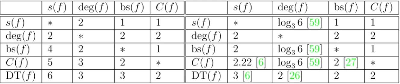
We summarize the current state of knowledge about these relationships in Table 2.1. Below, we list the facts that “generate” the left table, in the sense that any inequality implied by Table 2.1 can be proved by combining these inequalities in the proper sequence.

Fact 2.2.3. DT(𝑓 ) ≤ 𝐶(𝑓 )2 _{(Blum-Impagliazzo [}₈_])

𝑠(𝑓 ) ≤ bs(𝑓 ) ≤ 𝐶(𝑓 ) ≤ bs(𝑓 )2 _{(Nisan [}₆₀_])

bs(𝑓 ) ≤ deg(𝑓 )2 _{(Nisan-Szegedy [}₅₈_{], refined by Tal [}₇₃_])

DT(𝑓 ) ≤ bs(𝑓 ) deg(𝑓 ) (Midrijanis [55])

Fact 2.2.4 (Nisan, [60]). For monotone boolean functions 𝑓 , 𝑠(𝑓 ) = bs(𝑓 ) = 𝐶(𝑓 ) ≤ deg(𝑓 ).

Next we describe a construction of Wegener [75], which is a monotone function whose (block) sensitivity, degree, certificate and query complexity are all quite low compared to the number of variables. For each odd integer 𝑘 ≥ 1, we define the

3_{A number of other complexity measures, such as randomized and quantum decision tree}

com-plexities (with 0, 1 or 2-sided error) also fit into this “polynomial family”, but they do not play a significant role in this thesis so we do not define them here. These definitions can be found in [11], for example.

(20)

𝑠(𝑓 ) deg(𝑓 ) bs(𝑓 ) 𝐶(𝑓 ) 𝑠(𝑓 ) * 2 1 1 deg(𝑓 ) 2 * 2 2 bs(𝑓 ) 4 2 * 1 𝐶(𝑓 ) 5 3 2 * DT(𝑓 ) 6 3 3 2 𝑠(𝑓 ) deg(𝑓 ) bs(𝑓 ) 𝐶(𝑓 ) 𝑠(𝑓 ) * log₃6 [59] 1 1 deg(𝑓 ) 2 * 2 2 bs(𝑓 ) 2 log₃6 [59] * 1 𝐶(𝑓 ) 2.22 [6] log₃6 [59] 2 [27] * DT(𝑓 ) 3 [6] 2 [26] 2 2

Table 2.1: Best-known relationships (left) and separations (right) between complexity measures. On the left: A number 𝛼 in the row labeled by measure 𝐴 and the column labeled by measure 𝐵 means that for all boolean functions 𝑓 , 𝐴(𝑓 ) ≤ 𝐵(𝑓 )𝛼. So for example the 4 in the (bs, 𝑠) entry means bs(𝑓 ) ≤ 𝑠(𝑓 )4 for all 𝑓 . On the right: A number 𝛽 in the row labeled by measure 𝐴 and the column labeled by measure 𝐵 means that there exists (infinitely many) functions 𝑓 with 𝐴(𝑓 ) = ˜Ω(𝐵(𝑓 )𝛽). The corresponding reference is given in square brackets. For example, the 2 in the (bs, 𝑠) entry means we know of an explicit family of functions with bs(𝑓 ) = Ω(𝑠(𝑓 )2). Note that we do not include a column for DT(𝑓 ), since DT(𝑓 ) ≥ 𝐴(𝑓 ) for any measure 𝐴 considered here.

monotone address function

MAF𝑘 (︂ 𝑥1, . . . , 𝑥𝑘, {𝑦𝑆}_𝑆∈₍ [𝑘] ⌈𝑘/2⌉) )︂ := MAJ(𝑥1, . . . , 𝑥𝑘) ⋁︁ 𝑆∈₍_⌈𝑘/2⌉[𝑘] ₎ (︃ ⋀︁ 𝑖∈𝑆 𝑥𝑖∧ 𝑦𝑆 )︃ .

Proposition 2.2.5. The monotone address function 𝑓 = MAF𝑘 has 𝑠(𝑓 ) = bs(𝑓 ) =

𝐶(𝑓 ) = ⌈𝑘/2⌉ + 1, and deg(𝑓 ) = DT(𝑓 ) = 𝑘 + 1. Therefore, for 𝑚 ∈ {𝑠(·), bs(·), 𝐶(·)} and 𝑚′ ∈ {deg(·), DT(·)}, 𝑓 has 𝑛(𝑓 ) = Θ

(︂ 1 √ 𝑚(𝑓 ) · 4 𝑚(𝑓 ) )︂ = Θ (︂ 1 √ 𝑚′_{(𝑓 )} · 2 𝑚′(𝑓 ) )︂ relevant variables.

Proof. The fact that 𝑠(𝑓 ) = ⌈𝑘/2⌉ + 1 can be seen through a direct case analysis – we

refer the reader to the proof in [75] for details. By Fact 2.2.4, this implies the same for bs(𝑓 ) and 𝐶(𝑓 ). To compute deg(𝑓 ), note that we can write

MAF𝑘(𝑥, 𝑦) = ∑︁ 𝑆∈(_⌈𝑘/2⌉[𝑘] ) 𝑦𝑆 ∏︁ 𝑖∈𝑆 𝑥𝑖· ∏︁ 𝑖̸∈𝑆 (1 − 𝑥𝑖) + 1 (︃ _𝑘 ∑︁ 𝑖=1 𝑥𝑖 ≥ 𝑘/2 + 1 )︃ ⏟ ⏞ deg(·)≤𝑘 ,

and so each 𝑦𝑆 appears in a unique degree 𝑘 + 1 monomial 𝑦𝑆 · 𝑥1· · · 𝑥𝑘. Since DT(𝑓 ) ≥ deg(𝑓 ), and clearly DT(𝑓 ) ≤ 𝑘 + 1 (𝑓 can computed by querying the 𝑥 variables and then possibly the unique relevant 𝑦𝑆), it follows that DT(𝑓 ) = 𝑘 + 1 as well. The conclusion then follows from Stirling’s formula.

(21)

2.3 Improved bounds on the number of variables

2.3.1 Overview

Our goal is to generalize the ideas of Chiarelli, Hatami and Saks [13] to develop a unified framework for proving bounds on 𝑛(𝑓 ) in terms of various complexity measures like deg(𝑓 ), 𝑠(𝑓 ) and 𝐶(𝑓 ). The key player in each proof is a certain “coordinate version” 𝑚𝑖 of each complexity measure 𝑚, which is engineered to behave in a certain way with respect to restrictions of variables (see Definition 2.3.1). We call such 𝑚𝑖 “restriction reducing coordinate measures” (RRCMs) and form the corresponding potential functions

M(𝑓 ) := ∑︁

𝑖∈[𝑛]

𝛿𝑖(𝑓 )

2𝑚𝑖(𝑓 ). (2.12)

The defining properties of RRCMs are chosen to guarantee that, for any 𝐻 ⊆ [𝑛], M always obeys the inequality

M(𝑓 ) ≤ ∑︁

𝑖∈𝐻

𝛿𝑖(𝑓 )

2𝑚𝑖(𝑓 ) + E𝛼∼{0,1}

𝐻[M(𝑓_𝛼)]. (2.13)

This enables us to bound M(𝑓 ) recursively, assuming we choose the set of coordinates

𝐻 in such a way that the restrictions 𝑓𝛼 are guaranteed to have lower complexity, in some sense. Upper bounds on M(𝑓 ) naturally yield exponential upper bounds on 𝑛(𝑓 ) in terms of 𝑚(𝑓 ). We make these definitions precise below in the next subsection, and each subsequent subsection describes a different implementation of the general strategy above, yielding new bounds.

(22)

2.3.2 Restriction-reducing coordinate measures

Let us say a functional 𝑚 on boolean functions is an i-coordinate measure if 𝛿𝑖(𝑓 ) = 0 =⇒ 𝑚(𝑓 ) = 0.

Definition 2.3.1. We say an 𝑖-coordinate measure 𝑚𝑖 is restriction reducing if, for

any 𝑗 ∈ [𝑛] ∖ {𝑖}, and each 𝑏 ∈ {0, 1} : (1) 𝑚𝑖(𝑓𝑗=𝑏) ≤ 𝑚𝑖(𝑓 )

(2) if 𝛿𝑖(𝑓 ) = 1 and 𝛿𝑖(𝑓𝑗=𝑏) = 0, then 𝑚𝑖(𝑓𝑗=1−𝑏) ≤ 𝑚𝑖(𝑓 ) − 1.

We denote by ℛ𝑖 the set of restriction reducing 𝑖-coordinate measures. We abuse notation sightly and write {𝑚𝑖} ∈ ℛ𝑖 to denote that 𝑚𝑖 ∈ ℛ𝑖 for each 𝑖 ∈ [𝑛]. Properties (1) and (2) were essentially chosen to make the following a fact:

Fact 2.3.2. Let 𝑚𝑖 ∈ ℛ𝑖, and let 𝑗 ∈ [𝑛] ∖ {𝑖}. Then

𝛿𝑖(𝑓 )2−𝑚𝑖(𝑓 ) ≤

𝛿𝑖(𝑓𝑗=0)2−𝑚𝑖(𝑓𝑗=0)+ 𝛿𝑖(𝑓𝑗=1)2−𝑚𝑖(𝑓𝑗=1)

2 . (2.14)

Proof. If 𝛿𝑖(𝑓𝑗=0) = 𝛿𝑖(𝑓𝑗=1) = 1, then property (1) of Definition 2.3.1 implies that both 2−𝑚𝑖(𝑓𝑗=0) ≥ 2−𝑚𝑖(𝑓 ) _{and 2}−𝑚𝑖(𝑓𝑗=1) ≥ 2−𝑚𝑖(𝑓 )_{, which implies (}_2.14_{). Otherwise,}

suppose without loss of generality that 𝛿𝑖(𝑓𝑗=0) = 0 and 𝛿𝑖(𝑓𝑗=1) = 1. Then property (2) of Definition2.3.1implies that 2−𝑚𝑖(𝑓𝑗=1) ≥ 2·2−𝑚𝑖(𝑓 )_{which also implies (}_2.14_).

Fact 2.3.2 extends easily by induction to larger restrictions:

Fact 2.3.3. For any 𝑖 ∈ [𝑛] and any 𝐻 ⊂ [𝑛] with 𝑖 ̸∈ 𝐻, and any {𝑚𝑖} ∈ ℛ𝑖,

𝛿𝑖(𝑓 )2−𝑚𝑖(𝑓 ) ≤ E𝛼∼{0,1}𝐻

[︁

𝛿𝑖(𝑓𝛼)2−𝑚𝑖(𝑓𝛼) ]︁

. (2.15)

Proof. We proceed by induction on |𝐻|. The base case 𝐻 = {𝑗} is Fact 2.3.2. For the inductive step, observe that if 𝛿𝑖(𝑓 )2−𝑚𝑖(𝑓 ) ≤ E𝛼∼{0,1}𝐻

[︁

𝛿𝑖(𝑓𝛼)2−𝑚𝑖(𝑓𝛼) ]︁

(23)

all 𝑓 with 𝐻 = 𝐻1 or 𝐻2, then it holds for 𝐻 = 𝐻1⊔ 𝐻2, since 𝛿𝑖(𝑓 )2−𝑚𝑖(𝑓 ) ≤ E𝛼1∼{0,1}𝐻1 [︁ 𝛿𝑖(𝑓𝛼1)2 −𝑚𝑖(𝑓𝛼1)]︁ ≤ E𝛼1∼{0,1}𝐻1 [︁ E𝛼2∼{0,1}𝐻2 [︁ 𝛿𝑖(𝑓𝛼1,𝛼2)2 −𝑚𝑖(𝑓𝛼1,𝛼2)]︁]︁ = E𝛼∼{0,1}𝐻1⊔𝐻2 [︁ 𝛿𝑖(𝑓𝛼)2−𝑚𝑖(𝑓𝛼) ]︁ .

For any {𝑚𝑖} ∈ ℛ𝑖, we can define the associated potential function M via equation (2.12). By Fact2.3.3, M satisfies the inequality (2.13) for any set 𝐻 ⊆ [𝑛] of restricted coordinates. Next we introduce three explicit families of RRCMs, the first of which (deg_𝑖) was introduced in [13]:

Definition 2.3.4. For each 𝑖 ∈ [𝑛], define the 𝑖-coordinate measures

deg_𝑖(𝑓 ) := deg(𝑓 (𝑥) − 𝑓 (𝑥𝑖)) (2.16)

sens𝑖(𝑓 ) := max

{𝑥 :𝑓 (𝑥)̸=𝑓 (𝑥𝑖_)}𝑠𝑥(𝑓 ) + 𝑠𝑥𝑖(𝑓 ) (2.17)

cert𝑖(𝑓 ) := max

{𝑥 :𝑓 (𝑥)̸=𝑓 (𝑥𝑖_)}𝐶𝑥(𝑓 ) + 𝐶𝑥𝑖(𝑓 ) (2.18)

Lemma 2.3.5. For each 𝑖 ∈ [𝑛], the coordinate measures deg_𝑖, sens𝑖, and cert𝑖 all

belong to ℛ𝑖.

Proof. Since deg(·), 𝑠𝑥(·) and 𝐶𝑥(·) cannot possibly increase by restricting input vari-ables, property (1) of Definition 2.3.1 is trivially satisfied for each of the coordinate measures in question. To see that (2) holds, we abbreviate 𝑓𝑗=𝑏 by 𝑓𝑏 and assume without loss of generality that 𝛿𝑖(𝑓0) = 0.

First we argue that deg_𝑖(𝑓1) = deg𝑖(𝑓 ) − 1. We can write 𝑓 (𝑥) = 𝑥𝑗𝑓1(𝑥) + (1 −

𝑥𝑗)𝑓0(𝑥). Since 𝑥𝑖 does not appear in (1 − 𝑥𝑗)𝑓0(𝑥), it follows that 𝑓 (𝑥) − 𝑓 (𝑥𝑖) =

𝑥𝑗(𝑓1(𝑥) − 𝑓1(𝑥𝑖)) from which it is clear that deg𝑖(𝑓 ) = 1 + deg𝑖(𝑓1).

Next we argue sens𝑖(𝑓1) = sens𝑖(𝑓 )−1. Let 𝑥 be any input for which 𝑓 (𝑥) ̸= 𝑓 (𝑥𝑖), and let us write 𝑦 for the string which is 𝑥 with the 𝑗th bit omitted. Since 𝑓0 does not

(24)

so 𝑓1(𝑦) = 𝑓 (𝑥) ̸= 𝑓 (𝑥𝑖) = 𝑓1(𝑦𝑖). But then 𝑗 must be sensitive for 𝑓 at exactly one

of 𝑥𝑖 _{or 𝑥, hence 𝑠}

𝑥(𝑓 ) + 𝑠𝑥𝑖(𝑓 ) = 𝑠_𝑥(𝑓₁) + 𝑠_𝑥𝑖(𝑓₁) + 1.

Finally we argue cert𝑖(𝑓1) = cert𝑖(𝑓 ) − 1, which essentially follows from the previ-ous paragraph. Indeed, as above, all 𝑥 for which 𝑖 is sensitive for 𝑓 must have 𝑥𝑗 = 1, and 𝑗 must be sensitive for exactly one of 𝑥 or 𝑥𝑖 _{– suppose it is 𝑥 (wlog). Then any} certificate for 𝑓 which agrees with 𝑥 must assign 1 to 𝑥𝑗, since if it were allowed to be flipped, the certificate could not make 𝑓 constant. The claim follows.

Lemma 2.3.6. Let 𝑚𝑖 be a restriction reducing 𝑖-coordinate measure and set 𝑟 := min{𝑚𝑖(𝑥 ↦→ 𝑥𝑖), 𝑚𝑖(𝑥 ↦→ ¬𝑥𝑖)}. Then for any boolean function 𝑓 ,

𝛿𝑖(𝑓 )2−𝑚𝑖(𝑓 ) ≤ 2−𝑟· Inf𝑖[𝑓 ]. (2.19)

Hence M(𝑓 ) ≤ 2−𝑟_{· I[𝑓 ] and for any 𝑘 ∈ N, at most I[𝑓] · 2}𝑘−𝑟 _{relevant variables can}

have 𝑚𝑖(𝑓 ) ≤ 𝑘.

Proof. We proceed by induction on 𝑛(𝑓 ). If 𝑛(𝑓 ) = 1, then the corollary follows from

the definition of 𝑟 and the fact that Inf𝑖[𝑓 ] ≤ 1. Now suppose the desired inequality holds for all 𝑓′ with 𝑛(𝑓′) < 𝑛(𝑓 ), and we wish to show it holds for 𝑓 as well. Then by the induction hypothesis and Fact 2.3.2,

𝛿𝑖(𝑓 )2−𝑚𝑖(𝑓 ) ≤

2−𝑟· Inf𝑖[𝑓𝑗=0] + 2−𝑟· Inf𝑖[𝑓𝑗=1]

2 = 2

−𝑟_{· Inf}

𝑖[𝑓 ] (2.20)

where the final equality is Fact 2.2.1. If we sum this inequality over 𝑖 ∈ 𝑅(𝑓 ), we obtain M(𝑓 ) = ∞ ∑︁ 𝑘=0 |{𝑗 ∈ 𝑅(𝑓 ) : 𝑚𝑖(𝑓 ) = 𝑘}| 2𝑗 ≤ 2 −𝑟_{I[𝑓 ]} _(2.21)

which in particular implies that at most I[𝑓 ] · 2𝑘−𝑟 _{variables in 𝑅(𝑓 ) have 𝑚} 𝑖(𝑓 ) ≤

(25)

Observation 2.3.1. Applying Lemma 2.3.6 to the measures deg_𝑖 and sens𝑖 imme-diately yields both Nisan-Szegedy’s and Simon’s theorems. Indeed, min{deg_𝑖(𝑥 ↦→

𝑥𝑖), deg𝑖(𝑥 ↦→ ¬𝑥𝑖)} = 1 and min{sens𝑖(𝑥 ↦→ 𝑥𝑖), sens𝑖(𝑥 ↦→ ¬𝑥𝑖)} = 2, so

𝑛(𝑓 ) ≤ I[𝑓 ] · 2deg(𝑓 )−1 (2.22) 𝑛(𝑓 ) ≤ I[𝑓 ] · 4𝑠(𝑓 )−1. (2.23)

2.3.3 Degree

Let D(𝑓 ) := ∑︀ 𝑖∈[𝑛] 𝛿𝑖(𝑓 )

2deg𝑖(𝑓), and for any 𝐻 ⊆ [𝑛], let D(𝐻, 𝑓 ) =

∑︀ 𝑖∈𝐻

𝛿𝑖(𝑓 )

2deg𝑖(𝑓). For

any 𝑑 ∈ N, let D𝑑 = max{𝑓 : deg(𝑓 )≤𝑑}D(𝑓 ). In [13], the authors argue that one

can always find a set 𝐻 of ≤ deg(𝑓 )3 coordinates such that (i) deg_𝑖(𝑓 ) = deg(𝑓 ) ∀𝑖 ∈ 𝐻 and (ii) deg(𝑓𝛼) < deg(𝑓 ) for all 𝛼 ∈ {0, 1}𝐻. This implies D𝑑≤ 𝑑

3

2𝑑 + D𝑑−1, and hence that D(𝑓 ) < ∑︀∞

𝑑=1𝑑

3

2𝑑 = 26 for all 𝑓 . Combined with the observation

that D𝑑 ≤ 𝑑₂ (see Lemma 2.3.6), this yields Chiarelli, Hatami and Saks’ final bound

D(𝑓 ) ≤ 11 2 + ∑︀∞ 𝑑=12 𝑑 3 2𝑑 ≈ 6.614.

In this subsection, we implement their argument in a slightly different way to obtain a slightly stronger bound. In particular, rather than choosing 𝐻 to be a minimal set of coordinates which covers all max degree monomials in 𝑓 , we choose 𝐻 to be the variables in a single monomial of 𝑓 . Restricting this set of coordinates may not reduce the degree of 𝑓 , but as shown below, it will reduce the block sensitivity of

𝑓 . Hence, as we’ll want to induct on both degree and block sensitivity simultaneously,

we define

D𝑏,𝑑 := max 𝑓 with bs(𝑓 )≤𝑏

and deg(𝑓 )=𝑑

D(𝑓 ).

We also define 𝐵𝑑 := maxdeg(𝑓 )=𝑑bs(𝑓 ), and make the convention that D𝑏,𝑑 = 0 whenever 𝑏 > 𝐵𝑑.

Lemma 2.3.7. If 𝑀 is a monomial of degree 𝑑 = deg(𝑓 ) which appears in 𝑓 with

non-zero coefficient, then for any assignment 𝛼 : 𝑀 → {0, 1}, the restricted function 𝑓𝛼 has bs(𝑓𝛼) ≤ bs(𝑓 ) − 1.

(26)

Proof. Let us write any string 𝑥 ∈ {0, 1}𝑛 as 𝑥 = (𝑥𝑀, 𝑦), where 𝑥𝑀 ∈ {0, 1}𝑀 and

𝑦 ∈ {0, 1}[𝑛]∖𝑀_{. We claim that for any (𝑥}

𝑀, 𝑦), there is always a sensitive block for 𝑓 contained entirely in 𝑀 . Indeed, for any 𝑦, the function 𝑓 (·, 𝑦) has degree 𝑑, since nothing can cancel with the maximal monomial∏︀

𝑖∈𝑀𝑥𝑖. In particular, it is not constant, so for any input 𝑥𝑀, there is always at least one sensitive block for 𝑓 (·, 𝑦) at 𝑥𝑀. Therefore, bs𝑦(𝑓𝛼) + 1 ≤ bs(𝛼,𝑦)(𝑓 ), and the lemma follows.

Lemma 2.3.8. For each 𝑏, 𝑑 with 𝑏 ≤ 𝑑2_{, we have}

D𝑏,𝑑 ≤ 𝑑 · 2−𝑑+ max

𝑘∈{1,...,𝑑}D𝑏−1,𝑘

Proof. Suppose 𝑓 has deg(𝑓 ) = 𝑑 and bs(𝑓 ) ≤ 𝑏. Let 𝑀 be any degree 𝑑 monomial

in 𝑓 . Using (2.13), D(𝑓 ) ≤ |𝑀 | · 2−𝑑 ⏟ ⏞ = 𝑑·2−𝑑 + _E 𝛼∼{0,1}𝑀[D(𝑓𝛼)]. (2.24)

By Lemma2.3.7, each 𝑓𝛼 has bs(𝑓𝛼) ≤ 𝑏 − 1. Since D𝑏,𝑑 is monotone in 𝑏 (for feasible

𝑏 ≤ 𝑑2_{), it follows that for each 𝛼, D(𝑓}

𝛼) ≤ D𝑏−1,𝑘, where 𝑘 = deg(𝑓𝛼). Taking the maximum over all values of 𝑘 ∈ {1, . . . , 𝑑} yields a uniform bound that holds for all restrictions 𝑓𝛼.

Corollary 2.3.9. For every 𝑓 , and every 𝑑 ≥ 1,

D(𝑓 ) ≤ ⎛ ⎝D_𝐵_𝑑_,𝑑+ (𝑑 + 1)𝐵𝑑+1 2𝑑+1 + ∞ ∑︁ 𝑘=𝑑+2 𝑘(𝐵𝑘− 𝐵𝑘−1) 2𝑘 ⎞ ⎠ (2.25) ≤ ⎛ ⎝D_𝑑2_,𝑑+ (𝑑 + 1)3 2𝑑+1 + ∞ ∑︁ 𝑘=𝑑+2 2𝑘2_{− 𝑘} 2𝑘 ⎞ ⎠. (2.26)

Lemma 2.3.8 yields explicit bounds on D𝑏,𝑑 for any finite (𝑏, 𝑑), which in turn yields an explicit bound on D(𝑓 ) for any 𝑓 via Corollary 2.3.9. Incorporating the influence bound D𝑏,𝑑 ≤ 𝑑₂, we build up a table of upper bounds 𝐷(𝑏, 𝑑) recursively,

(27)

using the rule 𝐷(𝑏, 𝑑) = ⎧ ⎪ ⎪ ⎨ ⎪ ⎪ ⎩ min{︁𝑑₂, max𝑘∈{1,...,𝑑} {︁ 𝑑 · 2−𝑑+ 𝐷(𝑏 − 1, 𝑘)}︁}︁ for 𝑏 ≤ 𝐵𝑑 0 for 𝑏 > 𝐵𝑑 (2.27)

Supposing 𝐵𝑑 = 𝑑2 and extracting bounds recursively already shows that D(𝑓 ) < 5.0782, but we can further improve this by obtaining sharper upper bounds on 𝐵𝑑. For values of 𝑑 ≤ 14 (which contribute the most to 𝐷(𝑏, 𝑑) anyway), we can obtain such bounds by manually checking feasibility of a certain linear program, as shown below. (This reduction is partially inspired by ideas of Nisan and Szegedy in [58].)

Fact 2.3.10. If there exists a function 𝑓 : {0, 1}𝑛 → {0, 1} of degree 𝑑 with block

sensitivity 𝑏, then there exists another function 𝑔 : {0, 1}𝑏 _{→ {0, 1} of degree ≤ 𝑑 with}

𝑔(0) = 0 and 𝑔(𝑤) = 1 for each vector 𝑤 of hamming weight 1.

Proof. If 𝑓 (𝑥) attains maximal block sensitivity at 𝑧, then 𝑓 (𝑥 ⊕ 𝑧) attains maximal

block sensitivity at 0, so without loss of generality we may assume 𝑧 = 0, and possibly replacing 𝑓 by 1 − 𝑓 we may also assume that 𝑓 (0) = 0. If 𝐵1, . . . , 𝐵𝑏 are sensitive blocks for 𝑓 at 0, then define

𝑔(𝑦1, . . . , 𝑦𝑏) = 𝑓 (𝑦1, . . . , 𝑦1 ⏟ ⏞ 𝐵1 , . . . , 𝑦𝑏, . . . , 𝑦𝑏 ⏟ ⏞ 𝐵𝑏 )

so that for each coordinate vector 𝑒𝑖, 𝑔(𝑒𝑖) = 𝑓 (1𝐵𝑖) = 𝑓 (0

𝐵𝑖_{) = 1.}

For any 𝑑 ≥ 1, define the moment map 𝑚𝑑: R → R𝑑 by 𝑚(𝑡) = (𝑡, 𝑡2, . . . , 𝑡𝑑).

Proposition 2.3.11. If there exists a degree 𝑑 function 𝑓 : {0, 1}𝑛 _{→ {0, 1} with}

block sensitivity 𝑏, then there exists 𝜏 ∈ {0, 1} such that the following set of linear inequalities has a solution 𝑝 ∈ R𝑑_:

⟨𝑝, 𝑚𝑑(1)⟩ = 1

0 ≤ ⟨𝑝, 𝑚𝑑(𝑘)⟩ ≤ 1 for each 𝑘 ∈ {2, . . . , 𝑏 − 1} (2.28) ⟨𝑝, 𝑚𝑑(𝑏)⟩ = 𝜏

(28)

𝑑 1 2 3 4 5 6 7 8 9 10 11 12 13 14

𝐵𝑑≤ 1 3 6 10 15 21 29 38 47 58 71 84 99 114 Table 2.2: LP bounds on block sensitivity for low degree functions.

Proof. If such an 𝑓 exists, then let 𝑞(𝑥1, . . . , 𝑥𝑏) = _𝑏!1 ∑︀𝜎∈𝑆𝑏𝑔(𝑥𝜎(1), . . . , 𝑥𝜎(𝑏)), where

𝑔 comes from Fact 2.3.10, and set 𝜏 = 𝑔(1, 1, . . . , 1). It is well known (see [11]) that there is a univariate polynomial 𝑝 : R → R of degree at most 𝑑 such that for any 𝑥 ∈ {0, 1}𝑏_{, 𝑞(𝑥}

1, . . . , 𝑥𝑏) = 𝑝(𝑥1 + · · · + 𝑥𝑏). For each 𝑘 ∈ {1, . . . , 𝑏}, 𝑝(𝑘) is therefore the average value of 𝑔 on boolean vectors with hamming weight 𝑘, so in particular 𝑝(𝑘) ∈ [0, 1]. We also know 𝑝(0) = 𝑔(0) = 0, 𝑝(𝑏) = 𝑔(1, . . . , 1) = 𝜏 , and

𝑝(1) = _𝑛1 ∑︀

𝑖𝑔(𝑒𝑖) = 1, and hence the coefficients of 𝑝 provide a solution to the set of linear inequalities.

Using the simplex method with exact (rational) arithmetic in Maple, we compute the largest 𝑏 for which the LP (2.28) is feasible for 1 ≤ 𝑑 ≤ 14, which yields upper bounds on 𝐵𝑑 for small 𝑑. These bounds are summarized in Table 2.2. Recomputing the table 𝐷(𝑏, 𝑑) with 𝐵𝑑 given by Table 2.2 for 𝑑 ≤ 14 (and 𝐵𝑑 = 𝑑2 for 𝑑 > 14), we can recompute the table as in (2.27) with these boundary conditions. This time

𝐷(302_{, 30) ≤ 4.4157 . . . , which implies}

D(𝑓 ) ≤ 4.4158 (2.29)

for all 𝑓 . If we incorporate the main result of Section 2.4, which implies that

𝐵_𝑑2− 𝐵𝑑≤ 2 3(𝑑

4_{− 𝑑}2₎

into the table 𝐷(𝑏, 𝑑), we obtain the slightly stronger result D∞ ≤ 4.3935, which

implies

(29)

2.3.4 Certificate complexity

Now let us define the analogous quantities for certificate complexity. Let C(𝑓 ) := ∑︀

𝑖∈[𝑛] 𝛿𝑖(𝑓 )

2cert𝑖(𝑓), and for any 𝐻 ⊆ [𝑛], let C(𝐻, 𝑓 ) =

∑︀ 𝑖∈𝐻

𝛿𝑖(𝑓 )

2cert𝑖(𝑓). For any 𝑑 ∈ N, we

also define C𝑑= max{𝑓 : deg(𝑓 )≤𝑑}C(𝑓 ).

Theorem 2.3.13. For any 𝑑 ≥ 1, C𝑑≤ 1₂.

Proof. Let 𝑓 be a boolean function with deg(𝑓 ) = 𝑑. For any certificate 𝐶 for 𝑓 , let 𝐻 be the set of variables fixed by 𝐶. It follows from (2.13) that

C(𝑓 ) ≤ C(𝐻, 𝑓 ) + E𝛼∼{0,1}𝐻[C(𝑓_𝛼)]. (2.30)

Since 𝐶 is a certificate, we know deg(𝑓𝛼) ≤ 𝑑 − 1 for all 𝛼, and deg(𝑓𝛼*) = 0 for some

𝛼* ∈ {0, 1}𝐻_{. So, C(𝑓}

𝛼*) = 0, and we can improve (2.30) to

C(𝑓 ) ≤ C(𝐻, 𝑓 ) +(︁1 − 2−|𝐶|)︁C𝑑−1. (2.31)

Now take 𝐶 to be the globally smallest certificate for 𝑓 , so that 𝐶𝑖(𝑓 ) ≥ 2|𝐻| for all

𝑖 ∈ 𝑅(𝑓 ), and in particular

C(𝑓 ) ≤ |𝐻| · 4−|𝐻|+(︁1 − 2−|𝐻|)︁C𝑑−1. (2.32)

Since 𝑐 · 2−𝑐 ≤ 1

2 for 𝑐 ≥ 1, inequality (2.32) implies that C𝑑≤ 𝛼 · 1

2 + (1 − 𝛼) · C𝑑−1

for some 𝛼 ∈ [0, 1]. Therefore if C𝑑−1 ≤ 1₂ for some 𝑑, then also C𝑑≤ 1₂. The theorem then follows by induction on 𝑑, noting that C1 = 1₄ < 1₂.

Since C(𝑥 ↦→ 𝑥1) = 1₄, Theorem2.3.13 cannot be improved by more than a factor

of 2. In any case, we have the following immediate corollary:

Theorem 2.3.14. For any 𝑓 , 𝑛(𝑓 ) ≤ 1 2 · 4

𝐶(𝑓 )_.

Finally, we use an implementation similar to the one above to give a proof of a stronger bound on 𝑛(𝑓 ) in terms of deg(𝑓 ) for monotone functions 𝑓 .

(30)

Proof. We let ̃︁D_𝑑 denote the maximum value of D(𝑓 ) over all monotone functions of degree at most 𝑑. Given a monotone 𝑓 of degree 𝑑, let 𝐻 be the variables fixed by any minimal 0-certificate 𝐶. By monotonicity, 𝑓 (0𝐻, 1_𝐻) ≡ 0, so by minimality of

𝐻, each 𝑖 ∈ 𝐻 must be sensitive for 𝑓 at the input (0𝐻, 1𝐻). Therefore restricting the variables in 𝐻 to 1 yields an OR function on 𝐻, and hence each 𝑖 ∈ 𝐻 has deg_𝑖(𝑓 ) ≥ |𝐻|. If we restrict all of the variables in 𝐻 so that one of the restrictions is constant, we get the analogue of (2.32):

D(𝑓 ) ≤ |𝐻| · 2−|𝐻|+(︁1 − 2−|𝐻|)︁̃︁D_𝑑−1. (2.33)

However, if we only restrict those variables 𝑖 in 𝐻 with deg_𝑖(𝑓 ) = 𝑑, we obtain

D(𝑓 ) ≤ |𝐻| · 2−𝑑+̃︁D_𝑑−1. (2.34)

Combining these two inequalities yields

̃︁ D𝑑≤ max 1≤𝑘≤𝑑 {︁ min(︁𝑘 · 2−𝑘 + (1 − 2−𝑘)̃︁D_𝑑−1, 𝑘 · 2−𝑑+̃︁D_𝑑−1 )︁}︁ . (2.35) Note that ̃︁D₁ =̃︁D₂ = 1

2, since the only monotone functions of degree exactly two are

AND2 and OR2. Starting with these values and using (2.35) to recursively compute

bounds on ̃︁D_𝑑, we find that D̃︁₃₀ ≤ 1.3243, and hence D(𝑓 ) ≤ 1.3243 +∑︀∞ 𝑑=31

𝑑

2𝑑 <

1.325.

Remark: In [13], a function of degree 𝑑 with 1.5 · 2𝑑_{− 2 relevant variables is} con-structed. Therefore, Theorem 2.3.15 implies that all monotone functions of a given degree have at least 11% fewer variables than do certain general functions of the same degree.

(31)

2.3.5 Sensitivity

Define S(𝑓 ) := ∑︀ 𝑖∈[𝑛] 𝛿𝑖(𝑓 ) 2sens𝑖(𝑓) and S(𝐻, 𝑓 ) = ∑︀ 𝑖∈𝐻 𝛿𝑖(𝑓 )

2sens𝑖(𝑓) for any 𝐻 ⊆ [𝑛]. In light

of the previous subsections, it seems natural to expect that one should be able to prove a bound S(𝑓 ) = 𝑂(1) for any 𝑓 using a similar inductive argument, thereby improving Simon’s theorem (in the same sense that [13] improved Nisan-Szegedy’s bound.) However, choosing a good 𝐻 to restrict for S is tricky business – neither choice from the previous two subsections will work in general here. Despite this challenge, we believe such a bound does hold, so we leave it as a conjecture and provide some evidence in favor of it below.

Conjecture 2.3.16. For any 𝑓 , 𝑛(𝑓 ) . 4𝑠(𝑓 )_{. More strongly, S(𝑓 )}_{. 1.}

Our first piece of supporting evidence for Conjecture 2.3.16 comes from a direct combination of (2.2.4) with Theorem 2.3.13:

Theorem 2.3.17. For any monotone 𝑓 , 𝑛(𝑓 ) ≤ 1₂ · 4𝑠(𝑓 )_.

Theorem2.3.17is especially interesting in light of the fact that the tightest known example in Simon’s theorem is monotone. Our next two pieces of evidence are corol-laries of the following lemma, which is essentially a consequence of Huang’s theorem.

Lemma 2.3.18. For any function 𝑓 , and any monomial 𝑀 appearing in 𝑓 , the

number of variables 𝑖 ∈ 𝑀 with sens𝑖(𝑓 ) ≤ 𝑘 is at most (𝑘 − 1)2. The same is true of

any 𝑀 with ^𝑓 (𝑀 ) ̸= 0.

Proof. Let 𝐵 = {𝑖 ∈ 𝑀 : sens𝑖(𝑓 ) ≤ 𝑘}, and let 𝑀′ ⊆ 𝑀 be a minimal monomial containing 𝐵, in the sense that no other monomial 𝑁 has 𝐵 ⊆ 𝑁 ⊂ 𝑀′_{. Let 𝛼}

be a partial assignment which sets all coordinates in [𝑛] ∖ 𝑀′ to arbitrary values in {0, 1}, and sets those in 𝑀′ _{∖ 𝐵 to 1. Consider the polynomial 𝑓}

𝛼, which depends only on the variables in 𝐵. If 𝑓𝛼 does not have full degree |𝐵|, this could only be because the term 𝑐𝑀′∏︀_𝑖∈𝐵𝑥_𝑖∏︀_𝑖∈𝑀′_∖𝐵𝑥_𝑖 cancelled with another term of the form

𝑐𝑁∏︀𝑖∈𝐵𝑥𝑖∏︀𝑖∈𝑁 ∖𝐵𝑥𝑖 when 𝑀′∖ 𝐵 was restricted to 1. But this could only happen if

𝐵 ⊆ 𝑁 ⊂ 𝑀′, which by minimality of 𝑀′ _{cannot happen. Therefore |𝐵| = deg(𝑓}

(32)

and by Huang’s theorem [40], deg(𝑓𝛼) ≤ 𝑠(𝑓𝛼)2. But since sens𝑖(𝑓 ) ≤ 𝑘 for each

𝑖 ∈ 𝐵, 𝑠(𝑓𝛼) ≤ max𝑖∈𝐵sens𝑖(𝑓 ) − 1 ≤ 𝑘 − 1, and hence |𝐵| ≤ (𝑘 − 1)2.

To prove the same for a monomial 𝑀 appearing in the fourier transform, we switch to ±1 notation and observe that if 𝑧 ∼ {±1}[𝑛]∖𝑀 _{is a random assignment to}

the variables outside of 𝑀 , then

E𝑧∼{±1}[𝑛]∖𝑀[𝑓̂︁_𝑧(𝑀 )2] = E_𝑧∼{±1}[𝑛]∖𝑀 ⎡ ⎢ ⎣ ⎛ ⎝ ∑︁ 𝑇 ⊇𝑀 ^ 𝑓 (𝑇 )𝜒𝑇 ∖𝑀(𝑧) ⎞ ⎠ 2⎤ ⎥ ⎦ = ∑︁ 𝑇 ⊇𝑀 ^ 𝑓 (𝑇 )2 ≥ ^𝑓 (𝑀 )2 > 0

and hence there exists some restriction 𝑓𝑧 : {±1}𝑀 → {±1} witĥ︁𝑓_𝑧(𝑀 ) ̸= 0. There-fore we can apply Huang’s theorem as above and reach the same conclusion.

As we show below, Lemma 2.3.18 implies a bound on the number of variables

𝑖 ∈ 𝑅(𝑓 ) with sens𝑖(𝑓 ) ≤ 𝑘. Unlike the bound 1₄I[𝑓 ] · 2𝑘 (from Lemma 2.3.6), this bound only depends on 𝑘, and not the (average) sensitivity of the function 𝑓 , and for

𝑘 ≪√︁I[𝑓 ] it says something much stronger.

Corollary 2.3.19. Let 𝑣 : N → N be any increasing function such that ∑︀∞ 𝑘=1

𝑘 𝑣(𝑘) =

𝐶𝑣 < ∞. Then any boolean function 𝑓 has at most 𝐶𝑣 · 𝑣(𝑘) · 2𝑘 relevant variables

with sens𝑖(𝑓 ) ≤ 𝑘. In particular, the number of such variables is 𝑂𝜖(𝑘2+𝜖2𝑘) for any

𝜖 > 0.

Proof. For simplicity we consider only 𝑣(𝑘) = 𝑘3_{, the same proof works in general.}

Let 𝑆 be any set with ^𝑓 (𝑆) ̸= 0, and let 𝑎𝑘 = |{𝑖 ∈ 𝑆 : sens𝑖(𝑓 ) = 𝑘}|. Then by Lemma 2.3.18, for each ℓ we have ∑︀ℓ

𝑘=2𝑎𝑘 ≤ (ℓ − 1)2. Note that the solution to the (integer) linear program

maximize ∞ ∑︁ 𝑘=2 𝑎𝑘 𝑘3 subject to ⎧ ⎪ ⎪ ⎨ ⎪ ⎪ ⎩ ∑︀∞ 𝑘=2𝑎𝑘= 𝑑 ∑︀ℓ 𝑘=2𝑎𝑘≤ (ℓ − 1)2 for all ℓ ≥ 1 (2.36)

(33)

occurs when as much weight is put on the lower values of 𝑘 as possible, which means setting 𝑎𝑘 = 2𝑘 − 3. Therefore, ∑︁ 𝑖∈𝑆 1 sens𝑖(𝑓 )3 = ∑︁ 𝑘≥2 𝑎𝑘 𝑘3 ≤ ∞ ∑︁ 𝑘=2 2𝑘 − 3 𝑘3 =: 𝑐 < ∞. By Parseval’s identity ∑︀ 𝑆⊆[𝑛]𝑓 (𝑆)^ 2 = 1, this implies 𝑐 ≥ ∑︁ 𝑆⊆[𝑛] ∑︁ 𝑖∈𝑆 1 sens𝑖(𝑓 )3 ^ 𝑓 (𝑆)2 = ∑︁ 𝑖∈𝑅(𝑓 ) Inf𝑖[𝑓 ] sens𝑖(𝑓 )3 (2.37)

On the other hand, by Lemma 2.3.6, Inf𝑖[𝑓 ] ≥ 2−sens𝑖(𝑓 ). Then

𝑐 ≥ ∑︁ 𝑖∈𝑅(𝑓 ) 1 2sens𝑖(𝑓 )sens 𝑖(𝑓 )3 ≥ 1 𝑘3₂𝑘 · |{𝑖 ∈ 𝑆 : sens𝑖(𝑓 ) ≤ 𝑘}|, (2.38) from which the corollary follows.

A similar argument also works to show that S(𝑀, 𝑓 ) = 𝑂(1) for any monomial occurring in 𝑓 .

Corollary 2.3.20. For any function 𝑓 , and any monomial 𝑀 of degree 𝑑 in 𝑓 ,

S(𝑀, 𝑓 ) ≤ ⌊√𝑑+1⌋ ∑︁ 𝑘=2 2𝑘 − 3 2𝑘 + 𝑑 − ⌊√𝑑⌋2 2⌊√𝑑+2⌋ < 1.5.

Finally, we remark that most of the known functions4 _{with low sensitivity} com-pared to the number of relevant variables have the property that almost all of their variables never get to “interact” – that is, they are never simultaneously sensitive. Below, we give a simple tensorization argument which implies that any function 𝑓 with this property must obey the bound on 𝑛(𝑓 ) in Conjecture2.3.16.

Lemma 2.3.21. Suppose we can write 𝑅(𝑓 ) = 𝑌 ⊔ 𝑍, where for every input 𝑥, the

set 𝑠(𝑓, 𝑥) of sensitive coordinates for 𝑓 at 𝑥 has |𝑠(𝑓, 𝑥) ∩ 𝑌 | ≤ 1. Then |𝑌 | < 4𝑠(𝑓 )_.

4_{For example, the address function, the monotone address function, and the low-depth large-junta}

(34)

Proof. Replacing each 𝑦 ∈ 𝑌 with a copy of 𝑓 on 𝑛(𝑓 ) fresh variables 𝑥𝑦, we obtain a function 𝑓2with 𝑠(𝑓2) ≤ 𝑠(𝑓 )+𝑠(𝑓 )−1, since at most one of the 𝑦 variables and 𝑠(𝑓 )−1

other variables are sensitive in 𝑓 , which is really at most 𝑠(𝑓 ) “new” variables and

𝑠(𝑓 ) − 1 “old” variables in 𝑓2. Also, it is clear that 𝑛(𝑓2) = |𝑍| + |𝑌 |(|𝑌 | + |𝑍|) ≥ |𝑌 |2.

Recursively, we let 𝑓𝑘 be the function obtained from 𝑓 by replacing each 𝑦 ∈ 𝑌 with a copy of 𝑓𝑘−1 on fresh variables. By the same reasoning as the 𝑘 = 2 case, we see that 𝑠(𝑓𝑘) ≤ 𝑠(𝑓 ) + 𝑠(𝑓𝑘−1) − 1 ≤ 𝑘𝑠(𝑓 ) − 𝑘 and 𝑠(𝑓𝑘) ≥ |𝑌 |𝑘. If |𝑌 | ≥ 4𝑠(𝑓 ), then

𝑛(𝑓𝑘) ≥ 4𝑘𝑠(𝑓 ) = 4𝑘· 4𝑘𝑠(𝑓 )−𝑘 ≥ 4𝑘· 4𝑠(𝑓𝑘), which contradicts Simon’s theorem for 𝑘 large enough so that 4𝑘_{> 𝑘𝑠(𝑓 ) − 𝑘 ≥ 𝑠(𝑓}

𝑘). Therefore, |𝑌 | < 4𝑠(𝑓 ) as claimed.

2.3.6 Mixing measures

The goal of this subsection is to prove bounds on the number of relevant variables in terms of multiple complexity measures simultaneously, e.g.

𝑛(𝑓 ) . 2deg(𝑓 )2 +𝑠(𝑓 ). (2.39)

Note that such a bound would follow from taking the geometric mean of Theorem

2.3.12with Conjecture 2.3.16, however, we can give a direct and unconditional proof using the methodology we have already developed, combined with the following simple observation:

Observation 2.3.2. ℛ𝑖 is convex.

We therefore define, for any 𝛽 ∈ [0, 1], the coordinate measures 𝑑𝑠𝛽_𝑖, 𝑐𝑠𝛽_𝑖 ∈ ℛ𝑖 via

𝑑𝑠𝛽_𝑖(𝑓 ) := 𝛽 · deg_𝑖(𝑓 ) + (1 − 𝛽) · sens𝑖(𝑓 ) (2.40)

(35)

and the associated potentials DS𝛽(𝑓 ) := ∑︁ 𝑖∈[𝑛] 𝛿𝑖(𝑓 ) 2𝑑𝑠𝛽_𝑖(𝑓 ) (2.42) CS𝛽(𝑓 ) := ∑︁ 𝑖∈[𝑛] 𝛿𝑖(𝑓 ) 2𝑐𝑠𝛽_𝑖(𝑓 ). (2.43)

Proposition 2.3.22. For each 𝛽 ∈ (0, 1], DS𝛽(𝑓 ) = 𝑂𝛽(1). In particular, for 𝛽 = 1/2, DS𝛽(𝑓 ) < 8.277 for all 𝑓 .

Proof. Since 𝛽 > 0, we can essentially let deg_𝑖 do the legwork while sens𝑖 simply hangs on for a free ride. Indeed, let

DS𝛽_𝑑 := max

{𝑓 : deg(𝑓 )=𝑑}DS

𝛽_{(𝑓 )}

and suppose 𝑓 is any function of degree 𝑑. Let 𝐶 be any minimal certificate for 𝑓 , and let 𝐻 be the variables 𝑖 which are fixed by 𝐶. Let 𝐻′ ⊆ 𝐻 be those 𝑖 ∈ 𝐻 with deg_𝑖(𝑓 ) = 𝑑. Since any restriction 𝛼 of 𝐻′ lowers the degree of 𝑓𝛼, inequality (2.13) implies DS𝛽(𝑓 ) ≤ 𝑑 3 22−𝛽₍₂𝛽₎𝑑 + DS 𝛽 𝑑−1, (2.44)

where we have used that 𝑑𝑠𝛽_𝑖(𝑓 ) ≤ 2−𝛽𝑑−2(1−𝛽) for each of the variables 𝑖 ∈ 𝐻′, and that |𝐻′| ≤ 𝐶(𝑓 ) ≤ DT(𝑓 ) ≤ deg(𝑓 )3 _{by a result of Midrijanis [}₅₅_{]. By induction,}

we then have for all 𝑑 that

DS𝛽_𝑑 ≤ 𝑑 ∑︁ 𝑖=1 𝑖3 22−𝛽₍₂𝛽₎𝑖 < ∞ (2.45) which implies the desired conclusion with constant ₂2−𝛽1

∑︀∞ 𝑖=1 𝑖

3

(2𝛽₎𝑖, but this can be

im-proved dramatically. By Lemma2.3.6, DS𝛽(𝑓 ) ≤ ₂2−𝛽1 I[𝑓 ], so DS

𝛽_{(𝑓 ) ≤ min} 𝑘≥1{₂2−𝛽𝑘 + ∑︀ 𝑖≥𝑘+1 𝑖 3 22−𝛽₍₂𝛽₎𝑖}. For 𝛽 = 1

2, this minimum occurs at 𝑘 = 32, giving

DS12(𝑓 ) ≤ 1 21.5 (︃ 32 + ∞ ∑︁ 𝑖=33 𝑖3 2𝑖/2 )︃ = 11.602.

Assorted results in boolean function complexity, uniform sampling and clique partitions of graphs

Assorted results in boolean function complexity,

uniform sampling and clique partitions of graphs

by

Jake Wellens

Submitted to the Department of Mathematics

in partial fulfillment of the requirements for the degree of

Doctor of Philosophy in Mathematics

at the

MASSACHUSETTS INSTITUTE OF TECHNOLOGY

June 2020

c

○ Massachusetts Institute of Technology 2020. All rights reserved.

Author . . . .

Department of Mathematics

May 1, 2020

Certified by . . . .

Henry Cohn

Senior Principal Researcher at Microsoft Research New England and

Adjunct Professor of Mathematics at MIT

Thesis Supervisor

Accepted by . . . .

Jon A. Kelner

Chairman, Department Committee on Graduate Theses

Assorted results in boolean function complexity, uniform

sampling and clique partitions of graphs

by

Jake Wellens

Abstract

Acknowledgments

Contents

Chapter 1

Introduction

Chapter 2

On Some Extremal Properties of

Boolean Functions

2.1

Introduction

2.1.1

New Results

2.2

Preliminaries

2.3

Improved bounds on the number of variables

2.3.1

Overview

2.3.2

Restriction-reducing coordinate measures

2.3.3

Degree

2.3.4

Certificate complexity

2.3.5

Sensitivity

2.3.6

Mixing measures