ECOLE DE TECHNOLOGIE SUPERIEURE UNIVERSITE DU QUEBEC
THESIS PRESENTED TO
ECOLE DE TECHNOLOGIE SUPERIEUR E
IN PARTIAL FULFILLMENT OF THE REQUIREMENTS FOR THE DEGREE OF MASTER OF SCIENCE IN ENGINEERING
M. Eng.
BY
DE JESUS MOTA, Sandnne
IDENTIFICATION AN D VALIDATION O F A MODEL OF THE BELL-427 HELICOPTER FROM FLIGHT TEST DATA WITH A TIME-DOMAIN METHO D
MONTREAL, FEBRUARY 2 0 2009 © Copyright 2009 reserved b y Sandrine DE .lESUS MOTA
BOARD O F EXAMINERS (THESI S M . ENG. ) THIS THESIS HAS BEE N EVALUATE D BY THE FOLLOWING BOAR D OF EXAMfNERS :
Dr Ruxandra Mihaei a Botez, Thesis Superviso r
Department of Automated Productio n Engineerin g a t Ecole de technologic supcrieur e Dr Guy Gauthier, Jur y Presiden t
Department o f Automated Productio n Engineerin g at Ecole de technologic superieur e Joey Seto, Eng., External Jury Membe r
Senior Technical Specialis t (Aer o & HQ), Bell Hehcopter Textron Canad a
THIS THESIS HA S BEE N PRESENTED AN D DEFENDE D IN FRONT OF A BOARD O F EXAMINER S
ON 15 ™ OF DECEMBER 200 8
AKNOWLEDGEMENTS
1 would lik e t o expres s m y dee p gratitud e t o Professo r Ruxandr a Bote z wh o gav e m e grea t support throug h thi s thesis . Fo r th e las t year , sh e gav e m e th e necessar y resource s an d guidance t o progres s i n this research . Sh e gav e m e th e opportunit y t o b e mor e implicate d i n the aerospac e fiel d b y the several conference s w e participated .
I benefite d ver y muc h fro m th e assistanc e an d collaboratio n o f man y member s o f th e LARCASE tea m t o carr y o n ever y aspect s o f thi s thesis . Dr . Miche l Nadeau-Beaulieu , Mr. Andre i Popov an d Mr. Nicolas Boel y provided me great suppor t i n the methods use d and the goodnes s of the results. Mr. Sylvain Tetreaul t contribute d t o the compilation o f results. The wor k presente d i n thi s thesi s wa s par t o f th e CRIA Q 3. 4 projec t whic h wa s funde d b y Bell Helicopte r Textro n (BHT ) an d th e Consortiu m fo r Researc h an d Innovatio n i n Aerospace i n Quebe c (CRIAQ) . Additiona l scholarship s wer e obtaine d fro m Ecol e d e technologic superieure , which contribute to pursue this thesis without financial worries . Finally, las t bu t no t th e least, 1 would lik e t o thank m y family , Carlos , Fernanda an d Amelie , and m y boyfrien d Clemen t Rollie r fo r al l their lov e suppor t an d encouragement s throug h thi s research.
IDENTIFICATION E T VALIDATION D'U N MODEL E D E L'HELICOPTER E BELL-427 A PARTIR D E DONNEES D E VOL AVEC UN E METHOD E
TEMPORELLE DE JESUS MOTA, Sandrin e
RESUME
Une nouvell e techniqu e pou r I'identificatio n d'u n modcl e d'hclicopter e Bell-42 7 es t presentee. L e model e es t identifi e e t valid e pou r 2 2 condition s d e vol , chacun e etan t defmi e par un e altitud e varian t d e 300 0 pied s a 600 0 pieds , un e vitess e varian t d e 3 0 noeud s a 11 5 nosuds, un helicoptere lour d et un centre de gravite longitudina l etan t en avant et en arriere de rhelicoptere. Pou r identifie r le s modeles, de s commandes d e type 2-3-1- 1 son t executee s pa r le pilot e dan s l e bu t d'excite r tou s le s mode s d u systcme . Pou r identifie r l e mouvcmcn t longitudinal e t latera l d e I'helicoptere , u n nouvea u je u d e donnee s es t construi t e n concatenant le s donnee s reliee s a chaque command e d u pilote . L e model e construi t es t sou s la form e d'espac e d'eta t oi l le s vitesse s lineaire s e t angulaires , e t le s angle s d'Eule r representent le s etats du systeme et les accelerations lineaire s son t le s sorties du systemc . Deux problematique s majeure s son t resolue s dan s c e memoire . L a premier e concem e I'equation d'etat. Un e relation d e recurrence entr e le s etats est definie. Puis , une optimisatio n basee su r l a theorie de s reseau x d e neurones es t realisee e t un reglage manue l e t automatiqu e des condition s initialc s de s etat s es t fai t afi n d e satisfair e le s regie s d e l a FAA . L a sccond e problematique es t reliee a I'equation d e sortie. A cause des effets aleatoire s lor s de la prise de mesure, le s equations classique s d u mouvement n e donnent pa s de resultats satisfaisant s pou r observer le s sorties d u system e a partir de s etat s d u systeme . Deu x methodes (un e lineair e e t une non-lincaire ) son t presentee s e t un e comparaiso n de s troi s methode s es t realise e pou r determiner l a method e l a plu s appropriee . Dan s l e bu t d'effectue r un e comparaiso n propre , une list e de critere s es t forme e don t chacu n es t associe a un coefficien t d e ponderatio n selo n son importance . Ave c cett e comparaison , le s sentiment s subjectif s d u pilot e son t pri s e n compte.
Chaque model e identifi e a un e conditio n d e vo l doi t etr e valid e pa r troi s different s test s d e vol no n utilise s pou r I'identification . D e plus , chaqu e signa l estim e doi t reste r dan s l a band e de toleranc e defini e pa r l a FA A selo n l e typ e d e missio n d e I'helicoptere . Pou r le s test s d e validation, le s signau x estime s doiven t reste r dan s le s bande s d e toleranc e u n minimu m d e trois secondes .
De bon s resultat s son t obtenu s e n boucl e ouvert e e t e n boucl e ferme e pou r I'estimatio n de s signaux d'etat . L a method e lineair e s'es t avere e l a meilleur e pou r observe r le s sortie s d u systeme a parti r de s signau x d'etat . Le s matrice s obtenue s a chaqu e conditio n d e vo l son t interpolees pou r obteni r l e model e d e I'helicopter e pou r toute s le s condition s d e vol . Le s tests d e vo l no n utilise s pou r I'identificatio n e t l a validatio n d u model e son t utilise s pou r I'interpolation du modele. Les signaux estime s satisfon t le s regies de la FAA.
V
La generalisation d u modele pourrait etr e encore affinee c e qui permettrait d'implemente r l e modele dan s un simulateur , utilis e pou r I'entrainemen t de s pilotes e t de I'applique r comme base pour Fetude d'autres helicopteres.
IDENTIFICATION AN D VALIDATIO N O F A MODEL O F THE BELL-42 7 HELICOPTER FRO M FLIGH T DAT A TEST S WITH A TIME-DOMAIN METHO D
DE JESUS MOTA, Sandrin e ABSTRACT
A new techniqu e fo r th e Bell-42 7 helicopte r model identificatio n fro m flight dat a test s is here presented. A helicopte r mode l i s identifie d an d validate d fo r 2 2 flight conditions , whic h i s defined b y a n altitud e varyin g betwee n 3,00 0 f t an d 6,00 0 ft , a spee d varyin g fro m 3 0 knot s to 11 5 knots , a helicopte r loadin g wit h a heav y gros s weigh t an d a longitudina l af t an d forward cente r o f gravity . T o identif y th e models , 2-3-1- 1 multiste p contro l input s ar e perfonned b y the pilot t o excite all helicopter modes . In order to identify th e global motio n of the helicopter , a new dat a se t i s constructe d b y concatenatin g th e dat a relate d t o eac h o f th e four contro l inputs . The model i s represented i n the stat e spac e form wher e linea r and angula r velocities an d Eule r angle s ar e th e stat e variable s an d linea r acceleration s ar e th e outpu t variables.
Two majo r problem s ar e solve d i n thi s thesis. The first proble m concern s th e stat e equation . A recurrenc e relationshi p i s set up . Then, a n optimizatio n base d o n neura l networ k theor y i s performed an d a manual an d automati c tunin g o f th e initia l stat e condition s i s done i n orde r to satisf y th e FA A rules . Th e secon d proble m regard s th e outpu t equation . Becaus e o f random effect s whe n gatherin g data , classica l equation s o f motio n d o no t giv e goo d enoug h results t o observ e th e syste m output s fro m th e syste m states . Thus , tw o othe r method s (on e linear an d on e nonlinear ) ar e presente d an d a compariso n amon g th e thre e method s i s perfonned i n orde r t o find th e powerfu l method . T o realiz e a prope r comparison , a lis t o f criteria i s don e wit h weighte d coefficient s associate d t o eac h criterion . B y us e o f thi s comparison, subjectiv e feeling s o f the pilot are considered .
Each identifie d mode l i n a flight conditio n i s validated b y three differen t flight test s no t use d to identif y th e model . Then , eac h estimate d signa l ha s t o remai n i n a toleranc e margi n defined b y th e FA A accordin g t o th e flight missio n o f th e helicopter . Finally , fo r th e validation tests , estimate d signal s mus t b e withi n th e toleranc e margin s fo r a t leas t thre e seconds.
Good result s ar e obtained i n open-loop an d closed-loo p fo r th e state s identification . Th e bes t final scor e i s obtained wit h th e linea r metho d i n orde r t o observe th e syste m output s fro m it s states. Th e obtaine d matrice s ar e interpolate d t o obtai n th e mode l fo r an y flight condition . Flight test s no t use d fo r th e identification an d validatio n o f the model ar e used fo r th e mode l interpolation. Th e estimated signal s satisfy th e FAA rules .
The mode l generalizatio n coul d b e improve d i n orde r t o implemen t i t i n a simulator , whic h would be use for the pilot training, and apply it as a basis for other hehcopters study .
TABLE O F CONTENT S
Page INTRODUCTION 1
CHAPTER I SYSTE M IDENTIFICATIO N PROCES S 3 1.1 Definitio n 3 1.2 Manoeuvre s 4 1.2.1 Pilo t command 4 1.2.2 Fligh t missio n 8 1.2.3 Helicopte r loadin g 8 1.3 Measurement s 9 1.4 Mode l structur e 1 0
1.5 Identificatio n modellin g method s 1 0
1.6 Mode l constraint s 1 1 1.6.1 Toleranc e margins 1 1 1.6.2 Mode l performance 1 2 1.6.2.1 Th e correlation coefficient 1 2 1.6.2.2 Th e fit coefficient 1 3 1.6.3 Mode l plausibilit y 1 4
1.7 Question s raised i n this thesis 1 4
CHAPTER 2 STAT E EQUATIO N DETERMINATIO N 1 6
2.1 Formulatio n 1 6
2.2 Identificatio n o f the open-loop stat e equation by use of recursive method 1 7
2.2.1 Theor y 1 7
2.2.2 Practica l applicatio n 2 3
2.2.3 Result s for the flight conditio n HA6000ft-50kt s 2 4 2.3 Identificatio n o f th e closed-loo p stat e equatio n b y us e o f a n optimizatio n
procedure 2 7
2.3.1 Neura l network theor y 2 8
2.3.2 Algorith m applicatio n i n the project 3 4
2.3.3 Initia l conditions 3 5
2.3.3.1 Manua l tuning 3 6
2.3.3.2 Automati c tuning 3 7
2.3.4 Result s fo r th e flight condition HA6000ft-50kt s 4 2
2.4 Al l flight condition s synthesi s 4 3
CHAPTER 3 OUTPU T EQUATION DETERMINATIO N 4 5
3.1 Motivatio n 4 5
3.2 Nonlinea r metho d theor y 4 7
3.2.1 Subtractiv e cluster s 4 7
3.2.1.1 Parameter s definitio n 4 7
3.2.1.2 Standar d deviation 4 8
VIII
3.2.2 Linea r function betwee n th e input s and outputs dat a 5 4
3.2.3 Fuzz y syste m training 5 5
3.3 Linea r metho d theor y 5 6
3.4 Practica l applicatio n 5 7
3.5 Result s 5 8
3.6 Compariso n betwee n th e three methods 6 0
3.6.1 Methodolog y 6 0
3.6.2 Result s for the flight conditio n HA6000ft-50kts 6 3
3.6.3 Result s fo r all flight condition s 6 7
CHAPTER 4 GLOBA L MODE L 6 9
4.1 Formulatio n 6 9
4.2 Result s fo r the flight conditio n HA6000ft-50kt s 6 9
4.3 Result s fo r al l flight condition s 7 4
4.4 Mode l interpolatio n 7 5
CONCLUSION 8 0
APPENDIX I STAT E EQUATIO N RESULT S 8 2
APPENDIX I I STAT E AND OUTPUTS EVOLUTIO N I N OPEN AN D CLOSED
-LOOP 8 6
APPENDIX II I COMPARISO N AMON G TH E THREE METHODS FO R THE OUTPU T
EQUATION 8 7
APPENDIX I V COMPARISON AMON G TH E THREE METHODS FO R THE GLOBA L
MODEL 8 8
APPENDIX V STATE S AN D OUTPUTS EVOLUTIO N FO R THE MODE L
INTERPOLATION 8 9
LIST O F TABLE S
Page Table 1. 1 Toleranc e margins accordin g to the parameters an d the flight missio n 1 2 Table 2.1 Mode l performance s fo r th e flight conditio n HA6000ft-50kt s 2 7 Table 2.2 Influenc e o f th e initia l stat e variable s o n th e numbe r o f poin t outsid e
the tolerance margins when a manual tunin g i s done (%) 3 7 Table 2. 3 Influenc e o f th e initia l stat e variable s o n th e numbe r (% ) o f point s
outside of the tolerance margins when an automatic tuning is done 4 2 Table 3.1 Percentag e (% ) o f point s outsid e th e toleranc e margin s fo r al l flight
conditions whe n classica l equation s ar e use d t o observ e th e linea r
accelerations 4 6
Table 3.2 Percentag e (% ) o f point s outsid e th e toleranc e margin s fo r al l flight conditions whe n a linea r bloc k i s use d t o observ e th e linea r
accelerations 5 6
Table 3. 3 Reductio n (% ) of the percentage o f points out o f the toleranc e margin s for al l flight condition s whe n linea r metho d i s use d t o observ e th e
linear accelerations 5 7
Table 3. 4 Percentag e averag e o f th e numbe r o f point s outsid e th e toleranc e
margins fo r th e output equatio n (% ) 6 0
Table 3.5 Lis t o f th e criteri a weight s fo r th e compariso n betwee n th e thre e methods i n orde r t o observ e th e output s variable s fro m th e stat e
variables 6 2
Table 3. 6 Scor e (% ) obtaine d b y th e thre e method s fo r th e identificatio n o f th e flight conditio n HA6000ft-50kt s i n the output equatio n 6 4 Table 3. 7 Scor e (% ) obtaine d b y th e thre e method s fo r th e validatio n I o f th e
flight conditio n HA6000ft-50kt s i n the output equatio n 6 5 Table 3.8 Scor e (% ) obtaine d b y th e thre e method s fo r th e validatio n 2 o f th e
flight conditio n HA6000ft-50kt s i n the output equatio n 6 6 Table 3.9 Scor e (% ) obtaine d b y th e thre e method s fo r th e validatio n 3 o f th e
flight conditio n HA6000ft-50kt s i n the output equatio n 6 7 Table 3.10 Summar y of the three method goodnes s fo r the output equation (% ) 6 8
X Table 4.1 Table 4. 2 Table 4. 3 Table 4. 4 Table 4. 5 Table 4. 6 Table 4. 8
Percentage (% ) average s o f th e numbe r o f point s outsid e o f th e tolerance margin s fo r the global mode l 7 1 Score (% ) obtaine d b y th e thre e method s fo r th e identificatio n o f th e flight conditio n HA6000ft-50kts fo r th e global mode l 7 2 Score (% ) obtaine d b y th e thre e method s fo r th e validatio n I o f th e flight condifio n HA6000ft-50kt s fo r the global model 7 2 Score (% ) obtaine d b y th e thre e method s fo r th e validatio n 2 o f th e flight conditio n HA6000ft-50kts fo r th e global model 7 3 Score (% ) obtaine d b y th e thre e method s fo r th e validatio n 3 o f th e flight conditio n HA6000ft-50kt s fo r th e global model 7 3 Summary o f the three method goodnes s for th e global model (%) 7 4
LIST OF FIGURES
Page Figure 1. 1 Localizatio n of the commands in a helicopter 5
Figure 1. 2 Contro l inputs 5
Figure 1. 3 Comman d pilot selection 6
Figure 1. 4 Exampl e of the effect o f the four concatenated commands 7 Figure 1. 5 Test s points studied 9
Figure 2.1 Simulatio n of the open-loop state equation 2 4
Figure 2.2 Pilo t inputs for the model identification 2 5
Figure 2.3 Stat e variables evolution in open-loop for the identification 2 5
Figure 2.4 Pilo t command for the validation 1 2 5
Figure 2.5 Stat e evolution in open-loop for the validation 1 2 5
Figure 2.6 Pilo t command for the vahdation 2 2 6
Figure 2.7 Stat e evolution in open-loop for the validation 2 2 6
Figure 2.8 Pilo t command for the validation 3 2 6
Figure 2.9 Stat e evolution in open-loop for the validation 3 2 6
Figure 2.10 Simulatio n of the closed-loop state equation 2 7
Figure 2.11 Neura l network architecture 2 8
Figure 2.12 Multi-outpu t and multilayer neural network architecture 2 9
Figure 2.13 Initia l state conditions optimization procedure 4 1
Figure 2.14 Stat e evolution in closed-loop identification 4 2
Figure 2.15 Stat e evolution in closed-loop for the validation 1 4 2 Figure 2.16 Stat e evolution in closed-loop for the validation 2 4 3 Figure 2.17 Stat e evolution in closed-loop for the validation 3 4 3
XII
Figure 3.1 Output s evolution with classical equations 4 5
Figure 3.2 Subtractiv e clustering estimation 5 3
Figure 3.3 Linea r equation estimation 5 5
Figure 3.4 Evolutio n of the output error during the training 5 6
Figure 3.5 Simulatio n of the output equation 5 8
Figure 3.6 Output s evolution for the model identification 5 9
Figure 3.7 Output s evolution for the model validation 1 5 9
Figure 3.8 Output s evolution for the model validation 2 5 9
Figure 3.9 Output s evolution for the model vahdation 3 5 9
Figure 4.1 Globa l model simulation 6 9
Figure 4.2 Outpu t evolution for the global model identification 7 0 Figure 4.3 Outpu t evolutions for the global model vahdation 1 7 0 Figure 4.4 Outpu t evolution for the global model validation 2 7 0 Figure 4.5 Outpu t evolution for the global model validation 3 7 0
Figure 4.6 Inpu t command used for the interpolation 7 6
Figure 4.7 Stat e evolution for the interpolation 7 6
ABBREVIATIONS BFGS Broyden-Fletcher-Goldfarb-Shann o
CG Cente r of Gravity
CL Closed-loo p
DOF Degre e Of Freedom
FAA Federa l Aviation Administration
KKT Karush-Kuhn-Tucke r
L / H / A / F Ligh t / Heavy / Aft / Forward MISO Multipl e Input Single Output MIMO Multipl e Input Multiple Output
NN Neura l Network
SYMBOLS AND UNITS A, B, C, D Ax, Ay, Ar Corr Cov coll deg deg/s e FIT ft ft/min ft/s ft/s-h
[n
Id in J lat long lb m n U U, V , w u p^q^r s ped Var X yr
X a (p,0,\i/ 1 M Superscripts A TMatrices describin g th e discrete state-spac e mode l Linear acceleration s
Correlation coefficien t Covariance
Collective comman d positio n Degree
Degree per secon d Error vecto r Fit coefficien t Feet
Feet per minut e Feet per secon d
Feet per secon d square d Altitude rat e
Inertia matri x Identity matri x Inch
Cost functio n
Lateral cyclic command positio n Longitudinal cycli c command positio n Pound Output numbe r State numbe r Theil's coefficien t Linear velocitie s Input vecto r Rates Second
Pedals command positio n Variance State vecto r Output vecto r Forgetting facto r Lagrangian paramete r Standard deviatio n Attitude angle s Learning rat e Momentum Esfimated Transpose
XV bubscnpt des in new old out real s Desired Input New valu e Old valu e Output Measured
INTRODUCTION
The increasin g nee d fo r high-performanc e aircraf t o r rotorcraf t ha s initiate d a highe r us e o f system identificatio n methods . Suc h mathematica l model s ca n b e conceive d fo r flight simulator, flight contro l syste m o r handlin g qualitie s applications . I n thi s thesis , a Bell-42 7 helicopter globa l model is built from flight tes t data.
Two problem s regardin g th e mode l structur e ar e solved . Th e first on e regard s th e mode l degree. Severa l author s i n th e literatur e sa y tha t conventiona l si x degree s o f freedo m (DOF ) models wer e adequat e t o describ e a rotorcraf t dynamic s unde r th e hypothesi s tha t th e helicopter i s a rigid body . Ca n the Bell-427 helicopte r b e considered a s a rigid body s o that a six DO F mode l i s sufficien t t o characteriz e it s dynamics ? T o comput e thi s model , a stat e space linea r syste m i s conceived. Th e state variables ar e the linea r an d angula r velocitie s an d the Eulc r angles . Th e collective , longitudina l cyclic , latera l cycli c an d pedal s pilo t control s are use d a s th e syste m inputs . Thi s stat e equatio n i s studie d i n open-loo p i.e . th e state s evolution i s a fianction of the measure d state s an d pilo t controls . A closed-loop stud y i s don e in order to define th e states evolution a s a function o f the pilot controls only . The last stud y is the mor e realisti c on e becaus e i n reality , onl y th e pilo t ha s a contro l o n th e helicopte r dynamics h e i s flying. Th e closed-loo p stud y i s se t u p wit h th e resuh s foun d i n open-loop . Then, a n optimizatio n base d o n neura l networ k theor y an d a manual an d automati c tunin g o f initial state s condition s ar e use d t o clea r th e syste m t o diverg e an d t o increas e th e mode l efficiency.
The secon d problem regard s the system output s which ar e the linear accelerations. Generally , the classica l equation s o f motions ar e use d t o describ e a system. However , thi s metho d doe s not giv e accurat e result s t o observ e th e syste m output s fro m th e stat e variable s s o tha t tw o methods ar e se t u p t o obtai n a powerfu l method . A linea r metho d an d a nonlinea r metho d based o n fuzz y logi c ar e used . T o properl y compar e th e result s obtaine d wit h th e thre e methods (classical , linea r an d nonlinear) , a lis t o f criteri a i s considered . Weight s ar e attributed t o each criterio n t o underline the importance o f all of them.
This procedur e i s followed fo r eac h flight condifion , whic h i s defined b y an altitude, a speed , a cente r o f gravit y positio n an d a helicopte r loading . Th e pilo t flies th e helicopte r fo r different mission s whic h ar e leve l flight, ascending , descending , an d autorotatio n flight. Level flight test s ar e use d t o identif y th e models . T o evaluat e th e qualit y o f th e models , th e Federal Aviatio n Administratio n (FAA ) establishe d rules . Fo r eac h variabl e an d mission , tolerance margin s ar e defined . I n orde r t o validat e th e identifie d model , th e mode l i s computed fo r anothe r set of data i n input. The model response s ar e compared t o the measure d ones. I f they are "too" different, the n the model i s not robust enoug h an d the model shoul d be again designed .
The las t ste p o f th e mode l identificatio n i s it s generalizatio n i n th e flight envelope . Indeed , the mathematica l model s ar e valid onl y fo r a specific flight conditio n s o that a n interpolatio n between eac h flight conditio n mus t b e don e i n orde r t o obtai n th e syste m characteristic s a t any flight condition . I n thi s thesis , a n interpolatio n betwee n th e studie d flight condition s i s done accordin g to the speed .
This thesi s i s organized a s follows : i n Chapte r 1 , a literature revie w o f syste m identificatio n process i s presented. A direct lin k between literatur e revie w an d the thesis problems i s set up. In Chapte r 2 , th e stat e equatio n i s determine d wit h a recurrenc e metho d i n open-loop . Th e model optimizatio n an d th e tunin g o f th e initia l condition s ar e the n describe d i n orde r t o define th e closed-loo p model . I n Chapter 3 , the outpu t equatio n i s presented. Th e theorie s o f the classica l equation s o f motions , th e fuzz y logi c nonlinea r metho d an d th e linea r metho d are detailed. Th e comparison between results obtained with the three methods i s presented. I n Chapter 4, the global model i s obtained by models interpolatio n a s function o f speeds. Due to space restraints , onl y result s obtaine d fo r th e flight conditio n HA6000ft-50kt s (heav y gros s weight, af t cente r o f gravity , altitud e o f 6,00 0 f t an d spee d o f 5 0 knots ) ar e shown . Th e results o f all flight condition s ar e put in appendix .
CHAPTER 1
SYSTEM IDENTIFICATIO N PROCES S 1.1 Definitio n
According t o Jategaonkar (2006) , syste m identificatio n i s the proces s o f determination o f a n adequate mathematica l model , describe d wit h differentia l equation s containin g unknow n parameters whic h hav e t o b e determine d fro m measure d dat a suc h tha t th e mode l respons e matches adequatel y th e measure d syste m responses . B y "adequately" , i t i s introduce d a notion fo r whic h n o "perfec t fit" woul d b e possible , a s fo r rea l case s o r products . Fo r thi s reason, th e Federa l Aviatio n Administratio n (FAA ) ha s se t u p rule s i n orde r t o defin e th e term "adequate" .
System identificatio n need s t o be followe d b y a ste p calle d "mode l validation " t o asses s th e model fidelity . I f i t turn s ou t tha t th e identifie d mode l doe s no t mee t th e requirements , th e model structur e shoul d be changed an d the whole process shoul d b e repeated.
System identificatio n provide s a n overal l understandin g o f the flight vehicle' s dynamic s an d yields a n accurat e an d comprehensiv e dat a bas e fo r flight simulators , whic h ar e extensivel y used fo r pilot training and to minimize risk during experimental testing , which i s very costly . Hamel and Kaletka (1997 ) highlighted fou r importan t aspect s i n system identification :
(1) Th e maneuver. Th e input signal s have to be optimized i n their spectral composition i n order to excite all response modes fro m whic h parameters ar e to be estimated becaus e "If it is not i n the data, it cannot b e modeled" ;
(2) Th e measurements: Th e measurin g o f experimenta l dat a (i.e . fro m a rea l process) , sensors errors and measurement nois e complicate th e identification process ;
(3) Th e model structure: Dependin g o n th e mode l application , differen t structure s ca n b e chosen to describe the model ;
These four aspect s ar e usually calle d the "Quad-M" requirements . 1.2 Manoeuvre s
The dat a ar e sorte d b y differen t categories : (I ) the pilot command which ca n b e a collective, a longitudina l cyclic , a lateral cycli c o r a pedal control , (2 ) the fight mission whic h ca n b e a level flight, a n ascendin g flight, a descendin g flight o r a n autorotationa l flight, (3 ) tlie
helicopter loading dependin g on the gross weight an d the longitudinal cente r of gravity (CG),
(4) the attitude whic h varie s betwee n 3,00 0 ft an d 6,00 0 ft an d (5 ) the speed whic h i s between 3 0 knots and 11 5 knots.
In this section, th e way in which the flight tests data are sorted i s defined . 1.2.1 Pilo t comman d
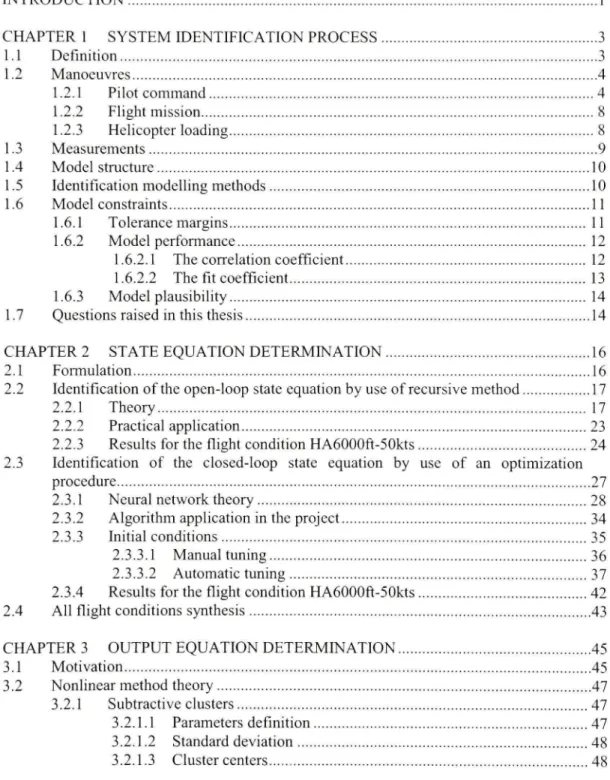
A pilo t manipulate s th e helicopte r flight control s i n orde r t o correctl y fly th e helicopter . A s previously said , four command s are used:
(1) Th e collective comman d change s angl e o f al l mai n roto r blade s a t th e sam e time an d independently o f their positions in order to control th e altitude;
(2) Th e longitudinal cyclic comman d varie s th e mai n roto r blade s pitc h i n orde r t o control the altitude o r to move forwar d o r backward ;
(3) Th e lateral cyclic comman d varie s th e mai n roto r blade s pitc h i n orde r t o mov e sideways;
(4) Th e anti-torque pedals comman d change s th e pitch o f the tail roto r blades , increasin g or reducin g th e thrus t produce d b y th e tai l roto r an d causin g th e nos e t o ya w i n th e applied pedal direction .
C'/clic stic k
Tail roto r pedal s
Collective leve r
Figure 1.1 Localizatio n of the commands in a helicopter. (http://community.bistudio.eom/wiki/Image:Helicopter-controls.jpg)
Gathered dat a basically limits, both in terms of scope and accuracy, the model developmen t and paramete r estimatio n wer e describe d (Jategaonkar , 2006) . On e o f th e mos t importan t aspects of data gathering is the choice of adequate inputs form to excite the aircraft motion in some optimum sense. Milliken (1951) presented the optimum input as the input which excites the best the frequency rang e of interest.
Generally, dynamic motion is excited by applying control pulse, step, multistep, or harmonic inputs. A variet y o f manoeuvre s wa s usuall y necessar y t o excit e dynami c motio n abou t different axe s using independent input s on every control (Jategaonkar, 2006). These differen t control inputs are presented in the following figure :
45 j 3 2 n Inpu t j
V
I Frequency SweepvA;Y«fp#-
it
Time I Time [s] [Pwbtct Ifiput j TimeFigure 1.2 Control inputs. From Hamel and Kaletka (1996), p. 263
The 3-2-1- 1 inpu t ha s a much wide r spectru m compare d t o the spectru m o f the impuls e or doublet inputs. The main advantage of the 3-2-1-1 input lies in its simplicity and its ability to manually realize it.
Two minor aspects of 3-2-1-1 inputs are:
(1) Their asymmetry about the trim deflection, an d as a consequence, they have nonzero energy at zero frequency;
(2) The first step being of larger duration, namely three units of A/ may lead to motions far from the initial trim condition before the application of following steps.
These undesirabl e effect s ca n be minimized b y modifying th e inpu t amplitude s o r by time twisting th e steps . Th e 2-3-1- 1 inpu t prevent s th e vehicl e fro m goin g fa r fro m th e tri m condition, before the application of the larger duration time step.
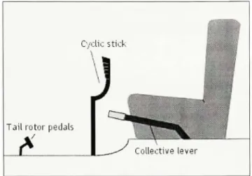
In orde r t o kno w whic h pilo t comman d i s relative t o a flight test, th e fou r command s ar e plotted which allows concluding the primarily command used by the pilot. Indeed, it is easy to distinguish a 2-3-1-1 command from another input type.
In the following figure, the flight test four controls are plotted:
»*^
n
"SS* :|-o -^-a n E -• E _ a ! •n-t, '^E s 1 1 1 1 ! 1 [ '- ^ 5 i ' Time[s| 1 1 1 1 I 1 • " • • ' ' \ ^ . > . — ^ ' ^ - v . ^ 1 1 1 1 1 1 lime[s] -—; ; ' ; ' • ' - ' ' " ' - ^ limelsl 1 1 1 1 1 1 1 ] 1 1 1 1 Time[s] ' -1 -1 1 1 1 -1 -1 1 , _ / / • ' - v 1 1 \ i 1 1 1 1 r Figure 1.3 Command pilot selection.By observing Figure 1.3 , there is no ambiguity about the pilot controls during this flight test. The pilot performed a collective command. The four step s with different tim e lengths for the 2 A?, 3 A/, A/ and A? of this command type are visible.
Is noted that the other commands ar e not constant during the flight test, which i s due to the high correlatio n betwee n al l helicopter comman d inputs . This ca n be explaine d b y the fac t that the aerodynamically behaviour of a helicopter cannot be split into to a longitudinal and a lateral motion as for an aircraft study .
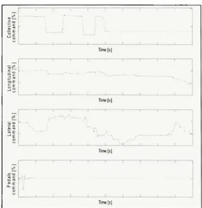
In orde r t o identif y th e helicopte r model , a ne w dat a se t i s constmcted . Th e fou r pilo t commands ar e concatenated s o that, for al l signals , the first quarter show s th e influence o f the collectiv e primar y control , th e secon d quarte r show s th e influenc e o f th e longitudina l cyclic control, the third quarter shows the influence o f the lateral cyclic control an d the last quarter shows the influence of the pedals control, please see next figure:
command comman d effect effec t
Pedals command
effect
1.2.2 Fligh t missio n
The flight mission s ar e split int o four categories :
(1) The Jlight level, whe n th e altitude rat e denote d b y h i s between -75 0 ft/min an d +75 0 ft/min. Th e altitude rate is defined b y the following expression :
[/; (flight test end)-/? (flight tes t start)]
''l„.„„„l = ^ x 6 0 ( l . l )
[flight test duration]. .
All flight test s whic h ente r i n thi s categor y ar e arrange d i n th e "Leve l Flight , ±50 0 ft/min" list .
(2) Th e ascending flight, whe n th e altitud e rat e i s higher tha n 75 0 ft/min. Al l flight test s entering into this category ar e arranged i n the "+1000ft/min" list .
(3) Th e descending flight, whe n th e altitude rate is lower than -75 0 ft/min an d the engines are on . Al l flight test s enterin g int o thi s categor y ar e arrange d i n th e "-lOOOft/min " hst.
(4) Th e autorotational flight, whe n th e altitud e rat e i s lowe r tha n -750ft/mi n an d th e engines ar e off . Al l flight test s enterin g int o thi s categor y ar e arrange d i n th e "Autorotation" list .
1.2.3 Helicopte r loadin g
Two parameter s mus t b e know n t o sor t th e flight tes t dat a accordin g t o th e hehcopte r loading:
(1) Th e gross weight whic h ca n b e "light " o r "heavy" . I f th e gros s weigh t i s lowe r tha n 5,600 lb , the n th e helicopte r i s considere d a s ligh t (L) . I f th e gros s weigh t i s highe r than 6,000 lb , then the helicopter i s heavy (H) ;
(2) Th e longitudinal center of gravity whic h can be "aft" o r "forward". I f the longitudina l center o f gravit y (CG ) i s fa r fro m th e helicopte r nos e tha n 22 4 in , the n th e longitudinal C G i s set to the aft (A ) of the helicopter. I f the longitudinal C G i s less fa r than 220 in, then i t is set to the forward (F ) of the helicopter .
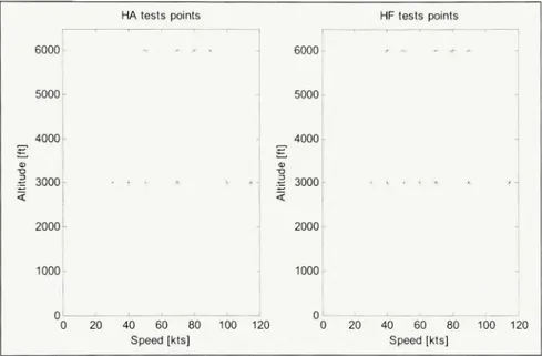
Thus, four conditions are presented: (L), (H), (A) and (F). Four combinations are considered in order to study the aerodynamically behaviou r o f the helicopter: HA , HF, LA and LF . In this thesis, only the results obtained fro m H A and HF flight conditions fo r altitude s varying from 3,000 ft to 6,000 ft are presented. The following figure shows the studied test points:
6000 5000 4000 ^. . | 300 0 < 2000 1000 0 -] 2 0 HA tests point s - . 40 6 0 8 0 Speed [kts] 100 1 6000 5000 4000 ^. a; . | 300 0 < 2000 1000 0 20 ) 2 0 HF tests point s ' - ^ • . . . . 40 6 0 8 0 Speed [kts] 100 -' 120
Figure 1.5 Tests points studied.
In thi s thesis , th e helicopte r i s modelin g fo r 2 2 flight condition s dependen t o n th e flight mission, helicopter loading, speed and altitude.
1.3 Measurement s
According t o Hame l an d Kaletk a (1997) , the measurement o f certain variable s depend s o n the model application an d the identification method . For some techniques, measurements of the stat e vecto r variable s ar e required . Accordin g t o th e mode l degree , a se t o f variable s needs t o b e measured . Fo r a si x DO F rigid bod y mode l identification , th e controls , th e speeds, the linear accelerations, the rates and attitudes must be measured.
10
1.4 Mode l structur e
The mode l structur e detemiine s th e difficult y degre e i n definin g th e unknow n parameters . According t o Tischle r an d Rempl e (2006) , th e rotary-win g aircraf t dynamic s ca n b e described wit h fou r mai n models :
(1) Th e quasi-steady lateral directional mode l (thre e DOF);
(2) Th e quasi-steady longitudinal mode l (thre e DOF) : Bot h thre e DO F model s ar e base d on the assumptions tha t longitudina l an d latera l directiona l degree s o f freedom ar e not coupled. I t coul d b e a goo d applicatio n fo r tilt-roto r an d th e tandem-roto r applications;
(3) Th e quasi-steady mode l (si x DOF) : I n thi s model , th e roto r steady-stat e respons e i s presented a s an equivalent quasi-stead y fuselag e derivative ;
(4) Th e hybrid fully coupled mode l (1 3 DOF) : Thi s mode l i s highl y accurat e fo r al l rotorcrafts.
According t o Hame l an d Kaletk a (1997) , mos t o f th e syste m identificatio n wor k wa s stil l devoted t o th e determinatio n o f parametric full y couple d si x DO F linea r derivative s models , which wer e considere d appropriat e fo r th e description o f the rigid bod y dynamics fo r th e lo w and medium frequenc y range .
1.5 Identificatio n modellin g method s
Two method s ar e mainl y use d t o identif y a model fro m flight dat a tests : a freqiiency-domam method, an d a /w/e-domai n method . A compariso n o f th e frequenc y an d time-domai n methods was given by Tischler an d Kaletka (1987) .
Frequency-domain identificatio n use d spectra l method s t o determin e frequenc y response s between selecte d inpu t an d outpu t pairs . Then , least-square s fittin g technique s wer e use d t o obtain closed-for m analytica l transfer-functio n linea r input-to-output models .
Time-domain identificatio n require d th e selectio n o f a state-spac e mode l structure , whic h may be linea r o r nonlinear . Mode l parameter s wer e identifie d b y least-squar e fittin g o f the response time-histories or by maximum likelihood methods.
Tischler an d Kaletk a (1987 ) presente d th e main advantage s an d inheren t limitation s o f the frequency an d time-domai n methods . Then , Tischle r an d Rempl e (2006 ) define d th e frequency sweep as the typical inpu t for frequency-domain an d the multistep inpu t for time-domain methods.
According t o Bohlin (2006) , three types of modeling methods existed: white box, grey box, and black bo x methods . Th e first categor y require d th e use r t o provid e th e equation s necessary to set up the model. This structure was very powerful whe n model was theoretical but i t di d no t giv e goo d resul t whe n th e environmen t gav e rando m effects . A t th e othe r extreme, the black box method could be used for any data type and without prior knowledge of the system dynamics. The weakness of this method is that the reproducibility of its results is doubtful. Th e grey box method is a mixture of both methods. Information abou t the whole system might be known, while relationships between subsystems are not known.
1.6 Mode l constraints 1.6.1 Toleranc e margins
In orde r t o evaluat e th e mode l goodness , FA A ha s define d rule s tha t describ e th e requirements to say that a model is "adequate". The estimated signal s must be found withi n the toleranc e margin s durin g a t leas t thre e seconds . Th e followin g tabl e regroup s th e parameters tolerance margins for various flight missions accordingly with the FAA rules.
12
Table l. l
Tolerance margins according to the parameters and the flight mission
Parameters States Outputs Variables u V w p q r <P
e
Ax A,. A, Flight mission Level Fligh t Descending Autorotation Tolerance margins ±5ft/s ± 4ft/ s ±3ft/s ± 3 deg/s ± 3 deg/s ± 3deg/ s ± 1.5de g ± l.5de g ± 3 ft/s' ± 3 ft/s' ± 3 ft/s' Flight mission Ascending Tolerance margins ± 5 ft/s ±4ft/s ±1.66ft/s ± 3deg/ s ± 3deg/ s ± 3deg/ s ± l.5de g ±3deg ± 3 ft/s' ± 3 ft/s' ± 3 ft/s' 1.6.2 Mode l performanc eIn order t o quantify th e model performance, tw o coefficients ar e calculated: th e correlation
coefficient which defines the trend of a signal, and the /?/ coefficient which measures the error
between the measured and the estimated signals.
1.6.2.1 Th e correlation coefficien t
The first metho d use s th e correlatio n coefficien t fo r th e mode l validation . Th e correlatio n coefficient Corr is given by the following equation:
Corr = Cov[y,y
,JVar{y)Var{y) (1.2)
where Cov is th e covariance , Var is the variance , y i s th e measure d outpu t an d y i s the estimated output.
13
The correlatio n coefficien t Corr equa l t o on e denote s perfect linear dependency (n o scatter ) between th e measured an d th e calculated o r estimated outputs . A correlation coefficien t equa l to minus on e (-1) denotes inverse linear dependency betwee n th e measured an d the estimate d outputs. A correlatio n coefficien t o f zer o denote s th e linear independency betwee n th e measured an d th e estimate d outputs . Th e correlatio n coefficien t compute s th e goodnes s o f the mode l i n a statistica l sense , bu t provide s littl e informatio n abou t th e mode l error . Mor e information abou t th e model error can be obtained b y the/// coefficient calculation .
1.6.2.2 Th e fit coefficien t
The Theil' s inequalit y coefficien t i s used t o define th e fit o f the estimate d signal s comparin g to the measured ones , and is defined a s follows :
F1T = \00{\-U) (1.3 )
Where:
-I(v,-7,r
U= . ' " ^ ' " , (1.4 )
f;Liy:yff,ny.)'
In Eq . (1.4) , th e variabl e > > represents th e estimate d signa l i.e . th e mode l output , y i s th e measured signal , i.e . th e rea l signa l an d s i s th e numbe r o f sample . Th e fit i s expresse d i n percentage, an d the t/coefficien t represent s th e ratio of the root-mean-square fit erro r and the root-mean-square value s o f the estimated an d measured signal s summe d together . It s value i s always foun d t o be between zer o an d one where zer o indicate s a perfect fit an d one the wors t fit.
Although th e acceptabl e valu e fo r U depend s i n th e application , i n general , a valu e i n th e range 0.25-0.3 indicate s a good agreemen t (Jategaonkar , 2006) .
14
1.6.3 Mode l plausibilit y
An over-parameterize d mode l wil l giv e a goo d respons e match , bu t no t necessaril y a goo d system representation . Th e mos t direc t wa y t o chec k th e plausibilit y o f th e estimate d parameters i s b y thei r comparison s wit h estimate s fro m othe r sources . Validatio n o n complementary dat a no t use d fo r th e estimatio n i s sometime s als o terme d loosel y th e "acid
test", an d ar e use d t o chec k th e mode l capability . I n mos t o f th e model validatio n exercises ,
including thos e fo r th e flight simulators , thi s approac h o f separatin g th e dat a fo r mode l development an d demonstratio n o f mode l fidelity i s adopted . Demonstratio n o f th e mode l fidelity o n complementar y dat a provide s increase d confidenc e i n th e mode l predictiv e capability.
For al l flight conditions , th e identifie d mode l i s validate d fo r three differen t flight tests , no t used t o identif y th e model . Differen t type s o f mission s ar e use d (whe n possible ) i n orde r t o validate th e longitudina l an d latera l motio n o f th e helicopter . I f the estimate d signal s remai n within the FAA tolerance margins , then the confidence i n the model capabilit y i s increased . 1.7 Question s raise d i n this thesi s
By analysi s o f th e overvie w o f syste m identificatio n presente d i n thi s chapter , tw o problem s related t o the Quad-Mare highlighted :
(1) Ca n th e dynamica l behaviou r o f th e Bell-42 7 helicopte r b e define d b y a si x DO F linear model ? Thi s proble m i s base d o n th e hypothesi s tha t th e helicopte r i s considered a s a rigid body .
This proble m i s related t o the model structure usuall y use d t o describe th e rigid bod y dynamics.
(2) Thre e method s (classica l equation s o f motion , linea r bloc k an d nonlinea r block ) ar e used t o estimate th e linear accelerations fro m th e stat e variables. Whic h metho d i s the most appropriat e t o give the best results ?
15
In order t o answe r thes e questions , a six DO F stat e spac e mode l i s built b y a //«;e-domain method. A compariso n betwee n result s obtaine d wit h th e thre e method s t o observ e th e system output s fro m it s state s i s then performed . I n case when th e estimated signal s satisf y the FAA rules, is concluded that model is well estimated.
CHAPTER 2
STATE EQUATIO N DETERMINATIO N 2.1 Formulatio n
Generally, a stat e spac e syste m wit h discret e dynamic s i s define d wit h th e followin g equation:
x{k + \) = A{k)x{k) + B{k)uik) (2.1 )
where xe 9^"an d w e 9?'" ar e th e stat e vecto r (x) an d th e inpu t vecto r (;/ ) which i s th e pilo t command vector . Matrice s A an d B are respectively th e "state matrix", the "input matrix" . The state variable s x ar e th e subse t o f syste m variable s tha t ca n represen t th e entir e stat e o f the syste m a t an y give n time . Th e state s variable s wer e chose n a s th e linea r an d angula r velocities u, v , w, p, q an d r an d th e Eule r angle s o f th e helicopte r aroun d th e X-axis an d Y-axis (Hame l et ai, 1996) , whic h ar e denote d b y f an d 6. Thes e variable s ar e sufficien t t o identify a rigi d bod y dynamic s o f a parametri c fully-couple d 6 DO F models . Th e headin g angle i/ / is dropped becaus e i t does not influenc e th e helicopter dynami c response .
The input variable s u are th e pilo t controls , whic h ar e th e collective , th e longitudina l cyclic , the lateral cyclic, and the pedals commands (se e Sectio n 1.2.1) .
Two method s ar e use d t o determin e th e A an d B matrices . First , a recursive metho d i s set u p to defin e th e matrice s i n open-loo p i.e . th e estimate d state s variable s ar e obtaine d fro m th e measured state s variable s an d th e pilo t commands . Then , a n optimization procedur e i s considered i n orde r t o obtai n th e optima l matrice s i n closed-loo p i.e . th e estimate d state s variables ar e obtained onl y from th e measured pilot commands .
17
2.2 Identificatio n o f the open-loop stat e equation b y use of recursive metho d 2.2.1 Theor y
For a discrete-tim e study , th e state s a t a sampl e tim e k depen d o n th e state s an d th e inpu t controls a t the previous sampl e tim e A- - 1 so that a recursive metho d ca n b e use d t o estimat e the A an d B matrice s (Jategaonkar , 2006) . As mentioned i n th e Sectio n 2.1 , th e state vector x and the controls vector u are defined a s follows :
x = \u v w p q r (j) 9^ (2.2 )
u = [coll long lat ped] (2.3 )
Then, 5 equations ar e considere d wit h {n + m) parameter s t o b e estimated . W e denot e b y n the numbe r o f state s variable s an d m th e numbe r o f pilo t commands . Th e k''' equatio n defining th e state element x, at step time k+ 1 is:
VA-e[l;.],V/4l;«],
The inpu t vecto r i s defined a s follows : VA-e|l;5|,
io{k)^[x{k) u{k)J (2.5 )
where io is a vector of dimensions [( « + w) x I)] .
The paramete r vecto r gather s th e element s o f A an d B matrice s an d i s forme d b y th e parameters t o b e estimated . Th e element s o f th e ;" ' lin e o f A an d B matrice s a t th e k''' ste p time are denoted a s follows :
V/tG l;.?IV/ e 1; «
ah{k)-[a•^ a., a 3 a.^ a.^ o, ^ o, , a ^ Z?, , 6, , 6, 3 /),_, ] (2.6 )
The / " stat e at the k''' sample tim e can be written, based o n Eqs. (2.4) and (2.5):
V A - G | 1 ; . | , V Z G | 1 ; « | ,
-v„/„(A- + l) = .v,„,(A- + l) + e(A-)
-v,.„(^ + l) = '^^,(A-)'o(A-) + e(A-) (2.7) where e is the error to be minimized .
For s measurements :
,v,(2) = afe,(l);o(l) + e,(l)
xfs)^abfs-l)io{s-\) + e, (s-l)
(2.8)
In Eq. (2.8), the initial conditions ar e represented b y the first sampl e tim e of zo vector. These 5 equations ar e summarized wit h the following formulation :
X,^^^AB.10 + e
Where:
(2.9)
^...(^) = [^...(2) .. . x,^{s)'J
/ 0 ( 5 - l ) - [ / o ( l ) .. . io{s-l)J
e{s-l) = [e{\) ... e{s-l)J
(2.10)
In order to minimize th e error, th e following cos t flinctio n J i s defined :
J{AB) = e^We
19
where W is a weighted matrix , which i s diagonal an d wher e th e no n diagona l elemen t ar e se t to zero . On e o f th e propertie s o f thi s typ e o f matri x i s tha t it s transpos e i s equa l t o itsel f i.e .
W = ^ . I f the diagonal term s w(k) ar e equal t o one, then th e error coefficients hav e the sam e
weight. I f not , the n i t mean s tha t th e erro r coefficient s ar e different . Deruss o et al. (1998 ) have chosen this weighted matri x s o that the A* element i s defined a s follows :
w{k) = r' (2.12
)
where y<\ i s a forgetting facto r an d s is the number o f measurements . Equation (2.11 ) becomes:
J{AB) = f^r'efk)
*=| (2.13 )
As s-k get s larger an d y does not equal to one, the weighting facto r approache s zero , therefor e older point s receiv e littl e weight . A s s-k goe s t o zero , th e weightin g facto r approache s on e and the most recen t dat a are favoured. Th e smalle r y is, the faster th e algorithm ca n track , bu t the mor e th e estimate s vary , eve n th e tru e parameter s ar e time-invariant . B y developin g th e cost function equation , we obtain :
J{AB) = e^fFe = ( X , „ - AB.IOf W (X^„ - AB.IO)
= XffVX,^^ - X^WABJO -{AB.Iof WX ^^.^ +{AB.10y WABJO (2.14 ) = Xl^WXj^^ - IXl^WAB.IO + lOfAB^W AB .10
The A an d B matrice s whic h minimiz e th e cos t functio n J ar e foun d b y equalizin g th e cos t ftjnction derivativ e with respect to AB t o zero:
dJ(AB)
— T - = ^
dAB
o -IX'^^W 10 + {I0.ABf W.IO + {IO.ABf W.lO = 0 (2.15 ) « - 2X',^^ W .10 + IIO'^W.IO.AB = 0
20
and next equation is obtained:
X^^W.fO = lO^W.IO.AB (2.16 )
The parameter vector is estimated as follows:
AB = [lO''WJO\' WW.Xj^ (2.17 )
The matrix /0(7V+1) can be written as:
IO{N + \) = [io{\) io{2) .. . /o(A ^ + l)7 ^2.18 )
-^TT
The term 10 W.IO o f the expression o f AB (se e Eq. (2.17)) i s developed b y introducin g a recurrence relationship:
10{N + \f W{N + \)IO{N + \) = Y,^o{k)w{k)io^ {k) =yio{k)f^'-'io'(k)
tt ^ ' ^
' (2.19
)
= j^io{k)rr"''io' {k) + io{N + \)/''*'^-^''^'^io'' {N + 1)
*- = n
^ylO''{N)W{N)IO{N) + io{N + l)io'{N + l)
The matrix P is defined as follows:
p-fk) = IO'{k)W(k)IO{k) (2.20 )
By substituting the expression of P' i n Eq. (2.19) for k = N, th e expression of P"' becomes:
p-'{N + \) = yP-'{N) + io{N + \)io''{N + \) (2.21 )
so that:
21
In order to obtain a recurrence expressio n o f P, th e following analytica l formul a i s used:
{A + BCDf' = A-'-A-'B[C-'+DA-'By' DA' (2.23)
By denotin g A = rP'fN),B = io{N+l),C = \,D = io'{N+\), th e expressio n o f P (A^ + I ) i s
rewritten as follows ;
P{N + \)- P(AO
7 _P{N)
7 -10 {N + [) l + /o^(/V + l)—^^;o(7V + l) 10 ^(A' + l)
P{N) (2.24)
With th e same reasoning, th e term 10 W.Xjes given by Eq. (2.17) is defined a s follows : / 0 ^ ( ^ + l)IT(yV + l)X,„,(A^ + l) = }'/0'(^)IT(Af)X,^(A^) + /o(A^ + l)x^„.(iV + l) (2.25 ) A new expression o f AB i s reformulated b y use of Eqs. (2.17) and (2.25):
/}5(7V+1): P(N\ P(N)
r r
)(Af + l) l + io' {N + l)-^—J-io{N + \) !0fN + \) P N] (2.26).[rlO'fN)W{N)X,jN) + io{N + \)x,jN+\)]
Hence, b y substitutin g Eq . (2.24 ) int o Eq . (2.26) , th e estimate d paramete r matri x i s define d as:
AB{N) = P{N)10'(N) W{N)Xj^^ [N) (2.27)
By developing Eq . (2.26 ) an d by replacing th e AB{N) formulatio n give n b y Eq. (2.27) , Eq. (2.26) becomes:
22
P(N)
AB{N + \) = AB(N) + —^^io{N + ]).x^^,^{N + \) 7 P{N) io(N + \) io{N + \) \ + io' {N + l)-^-^io{N + \) 7 x ^ ( A ^ ) . l + io'{N + \)-^—!-io{N + \) 7 io'{N + \)AB{N) .P(^) . X , ^ io'^{N + l)-^-^lo{N + l).x,.{N + \) 7 (2.28)
The K matrix i s defined as :
A'(jV + l) = - ^ - ^ / o ( A' + l) T, ^P{^) , (2.29) Then, Eq. (2.28) becomes:
PiN)
AB{N + \) = AB{N) + ^—^io{N + \)xj, {N + \)-K{N + \)io''{N + \)AB{N)
7 P(N) -K{N + \)io''{N + \)^-^io{N + \)x, (N + l) 7 (2.30) P{N)
By isolatin g ^/o(A ^ + l) o f Eq . (2.29) , an d replacin g it s expressio n i n Eq . (2.30) , th e
7
concise for m o f ^5(TV + 1) i s obtained:
AB{N + 1)^ AB{N) + K{N + l)[x,^,fN-^l)-io'AB{N)'j (2.31 )
By substituting Eq . (2.29) int o Eq. (2.24), the new expression o f P i s written as:
P{N + l) = -[f -K{N-\-l)io' {N + \)]P{N) (2.32)
The algorithm o f method implementatio n i n MATLAB / SIMULINK i s the following : (1) Initializatio n o f th e forgettin g facto r y s o tha t 0<y<\, whic h correspond s t o a n
exponential weighting . W e observ e tha t th e computatio n tim e decrease s b y keepin g y constant an d equa l t o one and does no t significantly affec t th e results.
23
(2) Initializatio n o f the matrice s P andAB wher e P i s chosen a s a diagonal matri x s o that its diagonal term s have high values and the AB element s ar e set to zero.
(3) Calculatio n o f the K matrix :
A:(A + l) = P(Ar)/o(A + l)[}'+/o^(A' + l)P(A)/o(A- + l ) j ' (4) Calculatio n o f the AB matrix :
AB (A -H) = AB{k) + K{k + l)[.v,„ (A +1) - io'' [k + \)AB{k)'\
(5) Calculatio n o f the P matrix :
P(A + l) = - [ / ^ - j ^ (A + l)/o^(A + l)]p(A)
(6) Computatio n o f th e thir d ste p an d repetitio n o f th e iteratio n procedur e fo r eac h sample time .
2.2.2 Practica l applicatio n
For th e open-loo p system , n o stat e feedbac k i s used. Th e stat e variable s ar e function s o f th e real stat e variable s an d pilo t control s a t th e previou s ste p time . Th e regressio n metho d described i n th e previou s sectio n i s use d t o estimat e th e stat e variables . Fo r eac h tim e step , the A an d B matrice s parameter s ar e obtained. Eac h coupl e o f matrices i s tested fo r th e entir e signals, an d th e couple s givin g th e bes t result s ar e selected . A n inde x wa s define d t o characterize th e matri x performance , an d i s use d i n th e flizz y logi c metho d t o find th e potential valu e of each point :
VA:€M%V/e]R",
pot{k) = Y.e - (2.33 )
The highes t thi s inde x is , th e bette r i s th e performanc e o f th e selecte d matrix . Sinc e th e matrix valu e was determined, th e state space dynamics i s time-invariant :
24
x{k + l)^Ax{k) + Bu{k)
and can be wriUen under the following form :
:{k + l)^[A B] .v(A)
u{k)
(2.34)
(2.35)
as shown in the following figure :
MEASURED STATES X{k) PILOT CONTROLS
.i(k + l •m Angular rates: [p q /• ] Linearvelocities: [ii v w]
.Eulerangles: [ ^ 6\
Figure 2.1 Simulation of the open-loop state equation. 2.2.3 Result s for the flight condition HA6000ft-50kt s
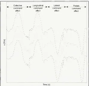
In this section, the plots of the states variables for one case study defined a s HA6000ft-50kt s are presented. The signals used to perform th e model identification ar e set up with four 2-3-1-1 concatenate d comman d pilot. The three validations used to validate the model are : (1) a 2-3-1-1 longitudina l comman d i n level flight, (2) no command i n a -1,000 ft/min flight, and (3) a 2-3-1-1 lateral command in level flight.
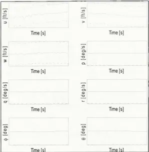
Figure 2.2 to Figure 2.9 show the pilot commands used to identify an d validate the model for this flight condition (lef t column ) an d th e stat e variable s evolutio n (righ t column) . For the figures o n the left side , the full blu e lin e are the pilot commands used for th e identificatio n and the dashed green lines are the pilot commands used to validate the model. For the figures on the right side, the full re d lines are the estimated states signals and the dashed black lines are the tolerance margins.
25
„ _ • > - a o '-4 | " 1 ^ >,3? •° E ^ F •— S ^ S E 5J E ui - O "- F Time (s] Time (s] 1 Time (s] , Time [s ]Figure 2.2 Pilot inputs for the model
identification.
CO ' 3 . w [fl/s ] o>^1
cn •& - -."^.Vr-Time [s] • , - - ~ - . - . _ . , . . ^ Time [s] Time [s] Time fsl g/s ] p [deg/s ] v [ft/s ] Time [s] Time [s]1
Time [s] Time fslFigure 2.3 State variables evolution in
open-loop for the identification .
Pedal s Latera l cycli c Longitidina l cycli c Collectiv e comman d (% ] comman d [% ] comman d (% ] comman d [% ] Time [s] 1 klentification Validation 1 • ' " ^ ' - • • " Time [s] ' • ' • Time (s] I •-- | 1 •nme [s] ij) [deg ] q [deg/s ] w [ft/s ] u [fl/s ] Time [s] -—'- '^ Time[s] Time [s] Time fsl Q . 03 CD T » Time [s] Time [s] , Time [s] Time fsl
Figure 2.4 Pilot command for the
26
cllv e an d [% ]11
tg
dina l man d :li c Longi l [% ] co m S""? Later a com m ^ Pedal s comman d Time [s] 1 Time [sj Time [s] Time [s| Identification Validation 2 1 " " " 1 j 1 i ' - • • ' i . ,11 [deg ] q [deg/s ] w [fl/s ] u [ft/s ] . , w -Time [s] Time (s) Time [s] Time fsl V [ft/s ] CO ap ] d r [deg/s ] • a CD Time [s] Time [s] Time [s] "lime tslFigure 2.6 Pilot command for the
validation 2.
Figure 2.7 State evolution in open-loop
for the validation 2.
^"? ^ F ° F " 1 o c t o ^ E cn O ° >."0 CJ c 2 E <D £ to o — - o n^e E o Time (s] Time [s] Tme [s) Time [s] Identificalion Validation 3 $ [deg ] q [deg/s ] w [fl/s ] u [ft/s ] ^'"~'., ' \ -Time [s] — ^-_._ ^ Time [s] Time [s] Time Isl e[deg ] r [deg/s ] p [deg/s ] v [ft/s ] _ - — - . > ^ . _ ^ •>•;,- -Time [s] Time [s] Tme [s ] Time tsl
Figure 2.8 Pilot command for the
validation 3.
Figure 2.9 State evolution in open-loop
for the validation 3.
Graphically, th e estimated signal s i n open-loop stud y respec t th e FAA tolerance margin s
during al l tim e histories . Th e fit and correlation coefficient s fo r thi s flight conditio n ar e
shown in the next table.
27
Table 2.1
Model performances fo r the flight condition HA6000ft-50kt s
Fit [% ] Correlation [% ] u 99.21 99.99 V 99.51 100 w 97.17 99.84 P 99.42 99.99 q 99.19 99.99 r 99.55 100 <P 99.49 100
e
99.38 99.99 For thi s flight condition , th e numerica l result s ar e ver y good . Th e fit an d correlatio n coefficients value s are higher than 97%. This model is identified and validated accordingly to the FAA tolerances margins rules.Moreover, al l the estimate d signal s sta y within th e tolerance margin s define d b y th e FAA, which increases the model goodness.
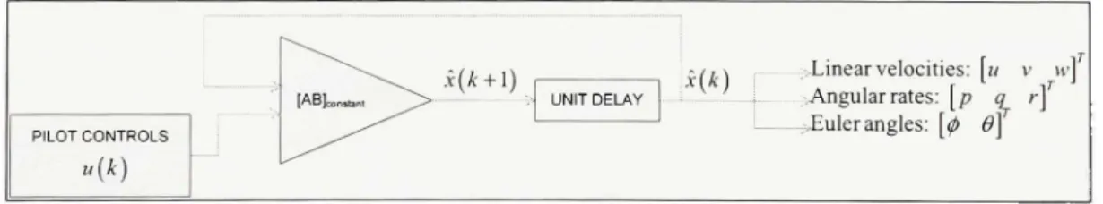
2.3 Identificatio n o f th e closed-loo p stat e equatio n b y us e o f a n optimizatio n procedure
For a closed-loo p simulation , a stat e feedbac k i s use d s o tha t th e onl y input s o f th e stat e equation are the pilot controls as shown in the following figure:
PILOT CONTROLS
u(k)
[ABU»» --.. i(/ t + l) UNIT DELAY
m1
.-..Linearvelocities: \u v w\ •Angular rates: \p q r ] - ;vEule r angles: [ ^ 6\
Figure 2.10 Simulation of the closed-loop state equation.
The A an d B matrice s foun d i n open-loo p d o no t guarante e goo d result s i n closed-loop . Indeed, a syste m i s stabl e i f an d eve n i f th e eigenvalue s ar e negativ e i f th e syste m i s continuous or if and even if the eigenvalues are inside an unitary circle centered on the plan origin i f the syste m i s discrete. When th e eigenvalues d o not satisf y thes e constraints , then the model is not stable, the responses tend to diverge. An optimization procedure is necessary
28
to obtai n goo d matrice s i n closed-loop . Th e open-loo p syste m matrice s ar e use d a s initia l guesses for the optimization.
The procedur e i s base d o n th e neura l network s theory . A mode l ca n b e idenfifie d b y providing a set of examples, i.e. input/target pairs of proper system behaviour (Haga n et al,
1996). A neural networ k i s composed o f element s operafin g i n parallel . Th e value s o f the connections betwee n the m ar e adjusted base d o n a comparison betwee n th e network outpu t and th e targe t (desired ) output . Thi s metho d i s calle d backpropagation and th e trainin g i s based on the Levenberg-Marquadt algorithm .
A second method used to satisfy th e project constraint s (see Section 1.6 ) i s the model tuning by adjustin g th e initial condifion s o f the system . Thi s techniqu e i s als o calle d a "proofof -match" of the model.
Thus, th e neura l networ k optimizatio n enable s th e syste m t o be stabl e an d th e "proofof -match" enables the estimated state parameters to match with the measured ones.
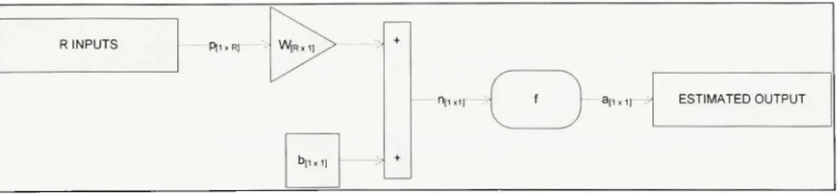
2.3.1 Neura l network theory
A neural network is composed o f an input p, a weight W, a bias b and a transfer functio n / called activation function a s shown below:
R INPUTS P|l, RI •\ W , R , ^ b|iKil + + — "11,11-^ 1 f a , , , , , - ^ ESTIIUIATED OUTPUT
Figure 2.11 Neural network architecture.
The mathematica l relationshi p betwee n al l thes e parameter s ca n b e formulate d a s i n Eq . (2.36):
29
a = f{Wp +
b)
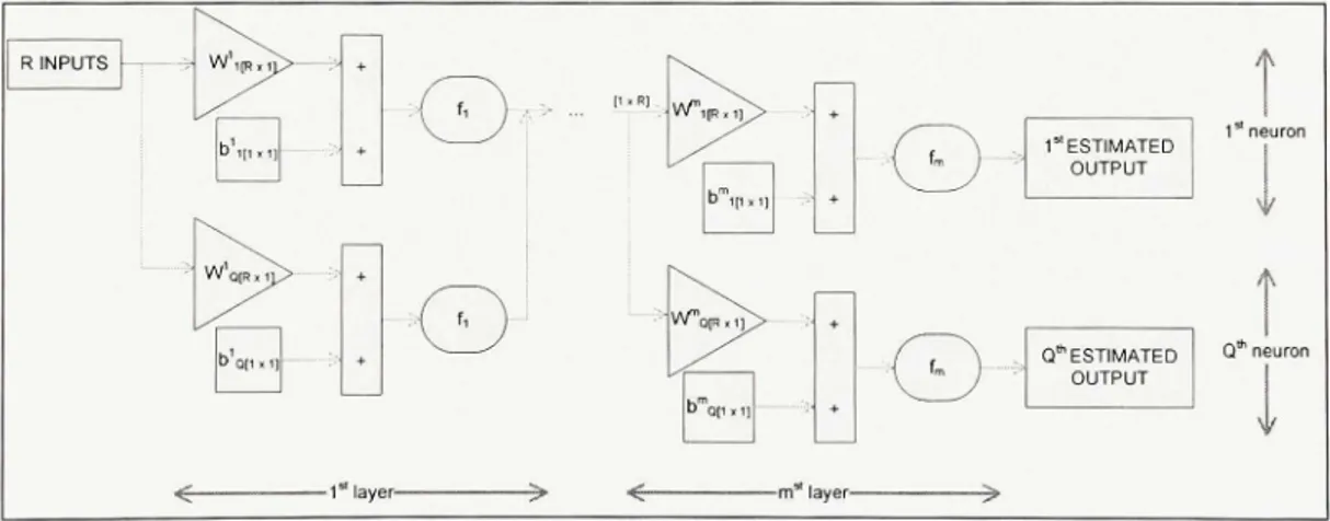
(2.36)In order to obtain an output a with Q elements i.e. a dimension [Q ^ X], Q neurons should be arranged in parallel. Therefore, the network can be composed by several layers in series, with different activatio n flinctions . Th e only constrain t fo r thes e fianction s i s that the y ar e to be
differentiable. For a multilayer network, Eq . (2.36) must be adapted i n order to consider all
activation functions . Fo r example, the equation relatin g the input and output o f a two-layer network {m = 2) with only one neuron {Q = 1) is:
a,^f,{w'p'+b') = f
w\f[w^p^+b^)yb'
(2.37)A neural network with several outputs and several layers is presented in Figure 2.12 :
R INPUTS -•-.• W',[R, r b\„,,: W^ofR.n, , + + - 1 ' ' layer — "" W",p,, ; b",,!,,, W ^ o p ^ b o[i)fi ] + -m layer —
o
1" ESTIMATED OUTPUTi
Q* ESTIMATED OUTPUTFigure 2.12 Multi-output and multilayer neural network architecture.
The backpropagafio n algorith m (Haga n et al., 1996 ) i s a gradien t descen t optimizafio n procedure i n whic h a mean squar e erro r performanc e inde x i s minimized b y adjustin g th e network parameters (weight s and biases). The performance inde x at iterafion k is defined a s follows:
30
F{w,b)=^-e'{k)e{k)^^-^[y,^S'^)-a{k)^[y,Jk)-a{k)] (2.38 )
where Vdes i s th e targe t outpu t an d a is th e neura l networ k outpu t whic h i s compare d t o th e desired output . Th e steepes t descen t algorith m considere d fo r th e approximat e mea n squar e error modelin g is :
Wf{k + \) = Wf[k)-q^ (2.39a )
aw^
b:'{k + \) = b'.:{k)-q^ (2.39b )
where m i s th e numbe r o f th e considere d laye r an d q i s the learnin g rat e calle d th e networ k training speed . Fo r a multilayer network , th e error i s an indirect functio n o f the weights i n the hidden layers , so that these derivatives are calculated differently :
dF dP dn" dw'" dn'" d vv, 'J dP dP du (2.40a) (2.40b) It is known that : m X ^ m m-\ , rm /'-\ A i \ ", = 2 J ^ , J ' ^ J +'' , (2.41 ) j=i
so tha t th e tw o derivative s — ^ an d - ^ ar e directl y define d sinc e th e ne t inpu t o f th e w * 3w" db"'
layer i s an explicit functio n o f the weights and biases in that layer :
dn"
d
m31
^ = 1 (2.42b )
db"-The P sensitivit y i s defined a s any effec t o f the syste m functio n o r any othe r syste m characteristic cause d b y a change i n on e o r mor e syste m parameters . Th e large r th e syste m sensitivity is , th e stronge r i s the effec t o f small change s i n the syste m performances . W e define:
dF
s"'=-^^ (2.43 )
' dn: ^
Then, Eqs . (2.40a) and (2.40b) become:
dF m m-X /' ^ / I * > \ s, a (2.43a ) d^^P dP ^ = s'" (2.43b ) db'" '
Thus, th e weigh t an d bia s expression s define d i n Eqs. (2.39a ) an d (2.39b ) ar e rewritte n as follows:
Wr{k + )) = Wf{k)-ns:a'f' (2.45a )
b';'{k + \) = b:'{k)-qs: (2.45b )
32
dnf
dn, -^ m + l - \ m + l 0/7, d/) |d
m "~ \ /? ;d
»/ + l - \ H J + I //, d« ,3
in ~\ nid
m + X dn',"a
ni + iffry
d
m on, dn dn'2 S"' m + t dn s"d
nd
n u.. (2.46)For one of the elements o f this above matrix, we can write:
du" .1 ^ "1 \r ^ '"+ 1 ' " , i,'"+ i A"'. ' ^1 +* '
d
nd
n n (2.47a)« ,„+ i da,
-w., dn"; " dn";
By according to Figure 2.11, a = f{n). Eq . (2.47 b) can be written i n the following for m
3«:"_ „.|3r(«; )
(2.47b)
By generalization o f these terms:
d m
d
n.m-d
n n d n f1. m + X rm I m\ (2.47c) (2.47d) dn" W'"*'F'"[n'") (2.48) where: F" = / " ( < ) 0 .. . 0 0 .. . 0 .. . 0 .. . 00 .. . 0 r[d"^)
(2.49)33
The recurrenc e relationshi p betwee n sensitivitie s a t differen t layer s i s writte n b y usin g th e chain nile : dP dP dn"
a
m ~\ m + l "- i m n an an m m + ]TTrni+\ j-.m ( m \ s = s W t UI \ (2.50)where m = M - 1 , ... , 2 , 1 and M i s the number of layers.
.M ,
The startin g point 5 (wher e M is the output layer ) i s defined wit h the recurrence relationshi p between sensitivities : .M _ dP an. M 1, d -«,)
[^<''
da. dn,~-S{t,
da, - - , ) da.'dnf
(2.51) Since:da, _aa;'_9r« )
M -\ M dn. dn, dn; : / - « ) (2.52)Next equatio n is written:
^-it,-a,)f"{n-)
(2.53)By summarizing , durin g th e first step , th e inpu t i s propagated forwar d throug h th e network . Then, durin g th e secon d step , th e sensitivitie s ar e propagate d bac k throug h th e network . Finally, during the third step, the biases and weights ar e updated .
![Figure 2.2 Pilot inputs for the model identification. CO ' 3 . w [fl/s] o> ^1 cn •& - -."^.Vr-Time [s] • , - - ~ -](https://thumb-eu.123doks.com/thumbv2/123doknet/7463480.222208/40.811.460.759.121.424/figure-pilot-inputs-model-identification-amp-vr-time.webp)