Science Arts & Métiers (SAM)
is an open access repository that collects the work of Arts et Métiers Institute of
Technology researchers and makes it freely available over the web where possible.
This is an author-deposited version published in: https://sam.ensam.eu
Handle ID: .http://hdl.handle.net/10985/16595
To cite this version :
Kwame ANANE-FENIN, Esther Tililabi AKINLABI, Nicolas PERRY - Quantification of nanoparticle dispersion within polymer matrix using gap statistics - 2019
Any correspondence concerning this service should be sent to the repository Administrator : archiveouverte@ensam.eu
Materials Research Express
PAPER
Quantification of nanoparticle dispersion within polymer matrix using gap
statistics
To cite this article: K Anane-Fenin et al 2019 Mater. Res. Express 6 075310
https://doi.org/10.1088/2053-1591/ab1106
PAPER
Quanti
fication of nanoparticle dispersion within polymer matrix using
gap statistics
K Anane-Fenin1
, E T Akinlabi1
and N Perry2
1 Department of Mechanical Engineering Science, University of Johannesburg, South Africa 2 Arts et Métiers ParisTech, CNRS, 12M Bordeaux, Esplanade des Arts et Métiers, France
E-mail:kwafen@ gmail.com
Keywords: agglomeration, dispersion, gap statistics, image segmentation, nanoparticles
Abstract
This study was prompted by the inadequacy of most dispersion quantification techniques to address
issues pertaining to scalability, implementation complexity, accuracy/error, uncertainty factors and
versatility. Therefore, a method for quantifying dispersion based on gap statistics was developed. A
dispersion quantity
(D) was formulated from a Gap factor ( )
G ,
0Particle spacing dispersity
(PSD
1) and
Particle size dispersity
(PSD
2) factors. The summation of the factors resulted in the dispersion
parameter
(D
p) which must be equal to one for an ideal or uniformly distributed condition. The state
of dispersion increases as
D→100%. The concept was tested with simulated models having uniform
dispersion, random dispersion, small aggregate, three large aggregate and one large aggregate were
successfully quantified to show 99.34%, 82.42%, 34.17%, 8.95% and 3.65% respectively. For
validation of concept, the state of dispersion when samples with
(scenario 1) and without (scenario 4)
silane treatment were quantified as 32,02% and 7.72% respectively. The concepts were then validated
using real microscopy images. This approach is robust, versatile and easy to implement.
Nomenclature
Acronyms
MeaningD dispersion quantity[%]
Dp dispersion parameter
G0 Gap Factor
PSD1 particle spacing dispersity PSD1 particle size dispersity
a initial inspected k-mean value or
b final inspected k-mean value
S Total interparticle spacing distance[pixels]
xi interparticle spacing
N number of particles
*
En expected value calculated from a reference distribution
k estimated optimal number of clusters
n sample size
Wk pooled within-cluster sum of squares around cluster mean
RECEIVED
25 November 2018
REVISED
14 March 2019
ACCEPTED FOR PUBLICATION
1. Introduction
There is increasing interest in polymer composite as an alternative to conventional material in the industrial sector due to the ease of manufacture, low cost and the possibility of optimising properties[1–5]. The superior benefits of polymer composites make the need for control and enhancement of its mechanical, physical and chemical properties imperative. There are several categories of polymer composites however, polymer nanocomposites are the most extensively researched as theyfind applications in multidisciplinary fields such as in drug delivery[1], purification systems [3], polymer biomaterials [4] and chemical protection [5]. The microscopic and mechanical properties of nanocomposites are significantly influenced by the nanoparticle dispersion quality[6]. The disparity between the experimental and theoretical tensile strength of
nanocomposites can be attributed to the inhomogeneous dispersion of the nano-reinforcement[6–9]. The possible states of dispersion are generally classified as either even, random or clustered [6,10]. However, an evenly and randomly dispersed state represents an optimal condition and usually correlates with enhanced properties. Achieving these optimal states is challenging, and has been reported as a significant limiting factor in nanocomposite fabrication[7,8,11]. The difficulty in achieving effective dispersion is attributed to the strong interparticle Van Der Waals forces which exceed the particle—matrix bond and consequently results in agglomeration[11]. Agglomerates resist intended property augmentation by compromising the mechanical integrity of the nanocomposite through void formations which are a source of crack initiation and possible failure during loading[7]. Therefore the need to improve dispersion and minimise agglomeration is vital to improving properties such as the mechanical(strength and stiffness) [12–16], thermal [17,18], electrical [14] barrier[19,20] and transparency [21]. Some of the techniques adopted for dispersion of nanofillers within the polymer matrix include mechanical or high-speed stirring[8], sonication [9,22], high shear mixing or melting [23,24], incorporating surfactants or compatibilisers [25] and casting solvents [26].
The traditional methods for assessing the state of nanoparticle dispersion is mostly qualitative via visual inspection of images from optical microscopy[25,27], Scanning electron microscope (SEM) [28,29],
Transmission electron microscope(TEM) [30,31] or Scanning probe microscope (SPM) [32,33]. Other direct approaches include Raman spectroscopy[34], UV-visible spectroscopy [35,36], electrical conductivity [8,23] andfluorescence [37]. These visual and direct approaches are often highly subjective and prone to errors and inconsistencies[38]. Therefore a quantitative means of assessment serves as an important step towards understanding the effects and relationships between the bulk scale functional performance and nanoscale structures of the nanocomposites[39]. Furthermore, quantification establishes a direct base for correlating the properties of the composite material to a standardised measure while providing the variables for
optimisation[16].
Some studies have been conducted in attempts to provide quantification techniques for assessing dispersion. Clark and Evans[40] quantified dispersion based on a randomly distributed determinant R. The distribution was considered random when R=1. The main drawback to this approach was the difficulty in selecting a reference sample for comparison. In a study by Moore[41] dispersion was assessed with three parameters namely; a variability index(VI), an anisotropic ratio (mean intercept size ratio) and a slice index which determines the degree of partteness.
Bakashi et al[39], developed two parameters for quantifying the state of dispersion. These were an image-based dispersion parameter(DP) and a clustering parameter (CP) derived via Delaunay triangulation. A satisfactory state of dispersion is realised when DP is high, and CP is low simultaneously. This method is only effective for comparing carbon nanotubes of similar concentration. Furthermore, the concept holds true only for regions of high CNT density.
Xie et al[31] characterised dispersion using a degree of dispersion (χ) and an average interparticle distance per unit volume(λV) of particles parameter. The degree of dispersion (χ) describes the percentage of clay exfoliation whileλVprovides a measure for the spatial separation of clay particles. Although the dispersion quantity generates distinguishing numbers, the information on the state of dispersion is not definitive.
The quadrant method has been extensively researched for quantifying dispersion[42–46]. Quantification is mainly based on the standard deviation of particle concentration within sections of the sample image. A higher standard deviation implies poor dispersion while the inverse is true. The main drawback to the quadrant method is in the selection of appropriate quadrant mesh size which can result in an unreliable and inconsistent
assessment.
In an attempt to improve upon the quadrant method, Michael and Raeymaekers[38] quantified dispersion by formulating of a composite index which comprised a dispersion and size distribution indexes. Their approach sought to improve on the limitations of the quadrant the method and succeeded in some respect, however, the inherent limitation of results depending on the quadrant to particle size was not eliminated.
Glaskova et al[20], proposed a premise that dispersion was a function of particulate area and a dispersion parameter(D). Where D was the probability of particles falling within a predetermined range of the particle area
distribution. An increase in D indicates an increase in inhomogeneity. The limitation of this method is that only a dispersion parameter is provided; however, an agglomeration parameter is absent.
Luo and Koo[47] presented a dispersion quantity (D) based on the integration of the probability density function(PDF) for estimating the statistical distribution of particle spacing (mean spacing (μ)). A Good dispersion was linked to high uniformity in the high spacing between integral bounds. The limitation of this approach is the sole reliance on free path spacing which implies that identical dispersion states may result regardless of the agglomerated group.
Tyson et al[48] improved on the approach of Luo and Koo [47] and developed two (2) quantities for assessing the state of dispersion. A dispersion quantity(D) was obtained by measuring the spacing between particles while the agglomeration quantity(A) was derived through particle size measurement. The disadvantage of this method is the challenge of selecting a correct distribution function.
Recently, Blazer et al[6], designed model based on interparticle distance, nanoparticle volume loading (f) andfibre-to-particle diameter ratios (D/d). A high value of the dispersion quality (β) indicates high dispersion state.
An approach for quantifying dispersion based on three main factors is presented.‘This study varies from other quantification techniques by being fundamentally based on the gap statistic for estimation of clusters, interparticle spacing and particle size disparities. Most of the literature for quantification of dispersion either do not consider an agglomeration factor or have separate values for dispersion and agglomeration. This method, however, provides an overall state of dispersion by incorporating free path spacing and an agglomeration component to comprehensively quantify the state of dispersion as a combined entity’. The dispersion percentage provide a scalable measure of the state of dispersion and serve as a standard for comparative analysis. The merits of the proposed techniques are critically analysed and characterized using model concepts and later validated with real images.
2. Materials and methods
In this study, two composites were plates manufactured from using titanium(IV) oxide nanoparticles (21 nm) and the silane coupling agent, 3-aminopropyltrimethoxysilane(APTMS), all acquired from Sigma Aldrich. Silane functionalization was conducted by mixing a solution of 95% methanol, 5% distilled water and 1% silane before the addition TiO2nanoparticle and heating at 95°C to ensure complete evaporation of the alcohol [49]. The mixture was dried at 100°C for 1 h and then crushed before dispersing via mechanical stirring within an epoxy matrix at a fraction weight of 2 wt%. Samples with and without silane treatment were mould. The TESCAN VEGA 3 XMU scanning electron microscope(SEM) equipment was used capturing the images and MATLAB for image analysis. The cross-section of the SEM samples was prepared by cryo-fracturing[50]. The samples were immersed in liquid nitrogen and then shattered. This method generally minimises distortions when compared to the use of shear force from a cutter. Sample sizes of approximately 5 mm lateral dimension were selected for experimentation.
3. Proof of concept
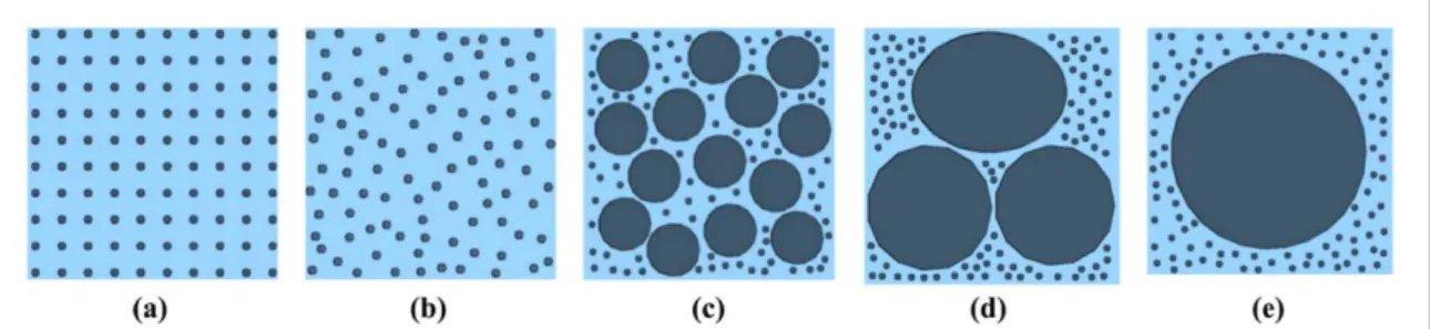
Five models simulating commonly occurring degrees of dispersion and agglomeration are presented for testing the concept. A uniform dispersion(Model 1), random dispersion (Model 2), random dispersion with small agglomerates(Model 3), random dispersion with three large agglomerates (Model 4) and random dispersion with one large agglomerate are described infigures1(a)–(e) respectively.
3.1. The gap statistic estimation
The Gap method proposed by Tibshirani et al[51] estimates the number of clusters within a data set and can incorporate almost all clustering algorithms such as the hierarchical or the K-mean for assessing changes in dispersion within clusters and a reference distribution. The number of clusters with the largest gap value is estimated when using the gap criterion. The optimal number of clusters is obtained from a tolerance range of the solution with the largest global or local gap value. The gap value is formulated as equation(1)
*
=
-( ) { ( )} ( ) ( )
Gap kn En log Wk log Wk 1 WhereEn*is the expected value calculated from a reference distribution using Monte Carlo sampling, n is the sample size, k is the estimated optimal number of clusters, and Wkis the pooled within-cluster sum of squares
around cluster mean or dispersion measurement. The drawback of the gap criterion is its expensive computation which is a direct consequence of applying cluster algorithms to reference data for all cluster solution[51].
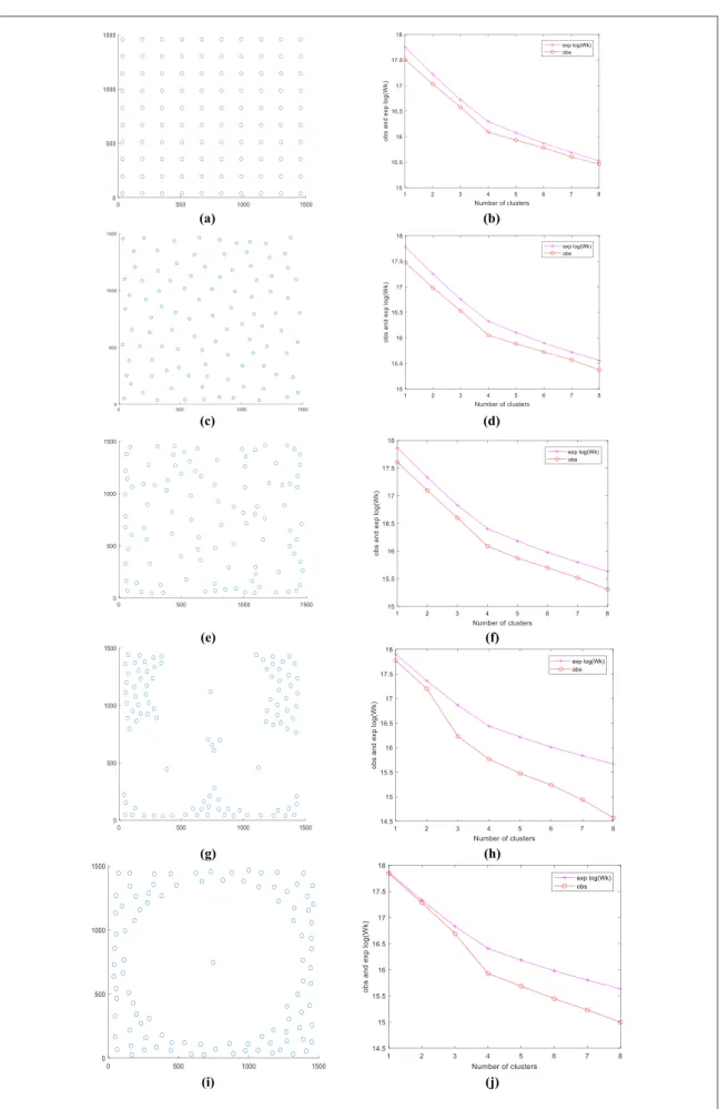
To obtain data for Gap factor analysis, the models were segmented using the K-means algorithm[52], transformed to binary images then the centroids of all segmented particles were extracted and plotted as described infigure2. The gap statistic criterion was applied to generate the observed and expected curves as shown infigure3.
The gap statistic curves observed infigure3clearly shows a widening as the level of agglomerates increase. This implies that the gap between curves for Model 5 is greater than that for Model 5. This trend in gap behaviour was used as a basis for formulating a gap factor (G0)illustrated infigure4and expressed in equation(2). The gap factor is, therefore, the difference between the area under the observed and expected curves.
ò
ò
= -= = ⎡ ⎣⎢ ⎤ ⎦⎥ ⎡ ⎣⎢ ⎤ ⎦⎥ ( ) ( ) ( ) G f x dx f x dx 2 a b e a b o 0 1 1WhereG0is the gap factor or area between the expected curve(f x( )e ) and observed curve ( ( )f xo) while the
initial andfinal inspected k−mean values are represented by a and b respectively.
To ensure accuracy in the obtained results, some assumptions and considerations were adopted.(1) Particle centroids were employed as a means for locating and extracting data from microscopy images.(2) To introduce standardisation, an equal number of particles were used and(3) all model images were converted to
1500×1500 pixels. (5) while an equal number of inspected k values [1–8] for the cluster analysis was implemented.
3.2. Particle spacing and size dispersity
To provide comprehensive quantification, two more factors namely; particle spacing dispersity (PSD1) and particle size dispersity(PSD2) were formulated to complement the gap factor. An algorithm was developed in MATLAB to calculate the minimum distance between all particles as the initial step for calculatingPSD1. For every point in boundary B, the distances to every point in boundary A were found as shown infigure5. All the distances(S) where calculated using equation (3).
= ( - ) +( - ) ( )
S Boundary Ax Boundary Bx 2 Boundary Ay Boundary By 2 3 Where x and y are the Cartesian locations and A and B represent two particle boundaries. The closest points, minimum distances and overall minimum distances were determined and used for the dispersity assessment.
Figure 1. Computer generated models for simulating possible particle distributions.(a) Model 1, (b) Model 2, (c) Model 3, (d) Model 4 and(e) Model 5.
Figure 3. Plotted centroids and corresponding Gap curves for Model 1(a) and (b), Model 2 (c) and (d), Model 3 (e) and (f), Model 4 (g) and(h) and Model 5 (i) and (j).
Similarly, the area of all the particles was used for calculating the particle size dispersityPSD2. The general expression for calculating the dispersity(PSD) is presented in equation (4).
å
å
å
=⎡ ⎣ ⎢ ⎢ ⎛ ⎝ ⎜ ⎞ ⎠ ⎟ ⎛ ⎝ ⎜ ⎞ ⎠ ⎟⎤ ⎦ ⎥ ⎥ ( ) PSD x x x N 4 i i i 2Where xiis the interparticle spacing or particle size while N is the number of variables(Particles). 3.3. Dispersion quantification
The dispersion quantity(D) shown in equation (5) was formulated based on a dispersion parameter (DP) which comprises the summation ofG ,0 PSD1andPSD2as expressed in equation(6). For an ideal condition such as a uniformly distributed system,D=100% andDP=3.This implies that Particle Size Dispersity, Particle spacing Dispersity and Gap factor each have a value=1.
=⎛ ´ ⎝ ⎜ ⎞⎠⎟ ( ) ( ) Dispersion Quantity D D 3 100% 5 P = + + ( ) DP G0 PSD1 PSD2 6 The quantified dispersion for the models is reported in table1.
Figure 4. Illustrations of the Area Under a Curve Method(AUCM) for dispersion quantification.
4. Results and discussion
4.1. Simulated models
The formulated dispersion quantity(D) was tested using the five simulated models. The resulting data was utilised to generate valuable characteristics such as average particle spacing and average particle spacing with their corresponding weighted averages and standard deviations for each model as presented in table1. The average particle spacing for Models 1,2 and 3 was similar and smaller than for Models 4 and 5. This observation correlates with the visual assessment as large aggregates were embedded in models 4 and 5. The spacing standard deviation for the uniform and randomly dispersed models(1 and 2) are smaller than the models with
agglomeration. The average particle size and standard deviations for Models 3–4 with agglomerates were greater than Models 1 and 2 which had same particle sizes.
The gap factor(G0), particle spacing dispersity and particle size dispersity for the uniform dispersion were 1,02, 1 and 1 which resulted in a dispersion(D) value of 99,34%≈100% that represents an Ideal state of dispersion. Model 5 had the worst dispersion state of 3,65%. From table2, the entire results indicate a decrease in dispersion percentage from Model 1 to 5 which was the expected trend from visual inspection. ThePSD1for Model 1 and Model 5 were 1 and 78,38 respectively. Furthermore, the most significant factor was the PSD2 which brings to for the importance of incorporating an agglomeration component for a comprehensive assessment of dispersion[48]. In theory, as D→100%, the state, of dispersion improves.
4.2. Validation using real images
The theoretical proof of concept has been established, however, validation using real SEM images was essential. Four SEM Images with different levels TiO2nanoparticles dispersed within the matrix as shown infigure6were used to test the concept. The state of dispersion was categorised into four scenarios to test the robustness and versatility of the approach. Every scenario underwent segmentation to highlight nanoparticle, conversion to centroid scatter plots and generation of gap statistic curves. The summary of results is presented in tables3and4. All image resolutions were converted to 1500×1500 pixels.
The analysis of the data for all four Scenarios is presented in tables3and4. The average particle spacing values were relatively similar for scenarios 1(7,40E+02), 2 (7,01E+02) and 3 (6,96E+02) however, for scenario 4, the average spacing(9,03E+02) was significantly higher in comparison. A high average spacing usually indicates the presence of large agglomerates. The standard deviation values did not show any significant variations. High average particle sizes values of 6,11E+02 and 2,44E+03 were observed for scenarios 1 and 4 respectively. Similarly, the standard deviations also showed higher values of 1,59E+03 and 1,76E+04 for Scenario 1 and 4 respectively.
A high average particle size and standard deviation value could indicate the presence of large agglomerates as in the case of scenario 4 or a sparsely dense particle distribution with relatively large size variations of smaller agglomerates as in Scenario 1. The above reasons shows that using just the particle spacing, particle size and standard deviations is not a sufficient enough approach for assessment of dispersion. These results confirm the finding of [47,51]. This study found that gap factor, particle spacing, and size dispersity are critical components of the dispersion parameter(Dp) for a comprehensive estimation of the dispersion quantity (D). The state of dispersion for Scenarios 1, 2, 3 and 4 were 31, 02%, 28, 60%, 22.95% and 7, 72% respectively. Scenario 1 was Table 1. Average particle spacing and size with corresponding standard deviations for the simulated models in pixels.
Model Ave. particle spacing Weighted average Std DEVIATION Ave. particle size Weighted average Std deviation
Model 1 7,84E+02 6,93E+02 3,75E+02 2,42E+03 2,43E+03 9,18E+01
Model 2 7,44E+02 8,06E+02 3,70E+02 2,42E+03 2,43E+03 9,18E+01
Model 3 7,71E+02 8,06E+02 4,07E+02 1,23E+04 7,12E+04 2,70E+04
Model 4 8,42E+02 1,11E+03 4,57E+02 1,45E+04 4,01E+05 7,52E+04
Model 5 9,14E+02 1,10E+03 4,59E+02 1,26E+04 9,89E+05 1,12E+05
Table 2. Degree of dispersion in the simulated models.
Model G0 PSD1 PSD2 Dp D
Model 1(Uniform Distr.) 1, 02 1 1 3, 02 99, 34%
Model 2(Random Distr.) 1, 56 1, 08 1 3, 64 82, 42%
Model 3(Small Agg.) 1, 93 1, 05 5, 8 8, 78 34, 17%
Model 4(Three Agg) 4, 49 1, 32 27, 7 33, 51 8, 95%
observed as the most homogenously dispersed while scenario 4 was the least homogeneous and highly agglomerated.
4.3. Influence of interparticle spacing and particle size
The elastic property of a nanocomposite is a function of particle size, weight fraction, particle contiguity, state of filler packing etc [53]. Particle distribution, contiguity and their interactions directly influence the
Figure 6. Data extraction process and Gap plots for real image scenarios 1, 2, 3 and 4.
Table 3. Average particle spacing and size with corresponding standard deviations for real image scenarios in pixels.
Real Images Ave. particle spacing Weighted average Std deviation Ave. particle size Weighted average Std deviation Scenario 1 7,40E+02 9,46E+02 3,46E+02 6,11E+02 4,65E+03 1,59E+03 Scenario 2 7,01E+02 6,40E+02 3,59E+02 6,67E+01 3,59E+02 1,94E+02 Scenario 3 6,96E+02 7,81E+02 3,94E+02 6,40E+01 5,05E+02 1,36E+02 Scenario 4 9,03E+02 1,25E+03 3,73E+02 2,44E+03 8,13E+04 1,76E+04
Table 4. Degree of dispersion for real image scenarios.
Real Images G0 PSD1 PSD2 Dp D
Scenario 1 0, 79 1, 28 7, 6 9, 67 31, 02%
Scenario 2 4, 21 0, 91 5, 37 10, 49 28, 60%
Scenario 3 4, 06 1, 12 7, 89 13, 07 22, 95%
thermomechanical properties of the nanocomposite[53]. Some have indicated that as the interparticle distance becomes smaller in comparison to the nanoparticle diameter, significant enhancement of mechanical properties such as toughness and stiffness takes place[54–56]. When such a condition occurs, a three-dimensional physical network often constructs within the interphase to dominate the nanocomposites performance[54,56].
However, this is only true for homogenously distributed nanoparticles as observed in table1, where both models 1 and 5 had smaller average interparticle spacings of 7,84E+02 and 9,14E+02 respectively than their
respective average particle sizes 2,42E+03 and 1,26E+04. The standard deviations of the average interparticle spacing show that model 1 with a smaller value of 3,75E+02 is more homogeneous than model 5 with
4,59E+02. Therefore, the role of interparticle spacing and particle size are critical for enhancing the mechanical properties of nanocomposites.
4.4. Particle matrix-interphase improvement
The particle matrix-interphase directly influence both particle distribution and contiguity. A critical assessment of the area surrounding an embedded particle within a matrix reveals a rather complicated phenomenon comprising shrinkage induced mechanical stresses, particle geometry induced even stress singularities or high-stress gradients, bonding imperfections, void contents and microcracks to mention a few[53]. Majority of the above-stated complex factors can be overcome by improving hydrophobicity of particles which minimises the occurrence of imperfect wetting. Therefore, the state of dispersion can be significantly improved by
functionalizing with oxidising agents and cavitation or ultrasonication dispersion which has proven to be an efficient approach [57–60]. Scenario 1, 2 and 3 which were selected from the silane functionalized sample and clearly showed better dispersion states due to better wettability from the silane treatment than Scenario 4 which was not treated. Hydrophobicity of the nanoparticles was achieved via the formation of afilm with Ti–O–Si chemical bonding and cross-linking bonds of Si–O–Si after the silane treatment [61].
5. Conclusion
A method was developed for deductively quantifying dispersion and agglomeration within particle reinforced polymer composites. The approach was successfully applied to simulated models and validated with SEM images. It was observed that for a comprehensive determination of the dispersion state of a system, the dispersion parameters, the gap factor, particle spacing and particle size dispersity are vital components as standard deviation data alone was not sufficient for accurate assessment. In theory, as (D) approaches 100%, the state of dispersion improves. The current technique is versatile and capable of analysing optical and electron microscopy images. The results can be used as a platform for introducing some measure of standardisation aimed at benchmarking dispersion quality. This proposed method can be modified to analyse 3D images with ease. The aim of the composite design is to manufacture superior performance materials using optimal parameters. This study has shown that optimisation of the degree of dispersion within composites is possible since a reliable numerical measurement for accurate quantification has been provided. The new approach avoids the limitations of previous methods such as the over-reliance on standard deviation, means and varied
probability distribution functions. Dispersion directly impacts the thermomechanical properties of nanocomposites, therefore as technology advances customising the state of dispersion to impart specific properties will become a reality and approaches such as in this study will be key for customisation of such nanocomposites. The dispersion quantity is easy to implement and execute and shows reliable and consistent outputs that are very similar to visual assessments. The formulation ensures robustness and some level of sophistication without the complexity of other methods. Furthermore, a stepwise increase in magnifications can be used to generate various images that can be employed to give a better representation of the dispersion state within the entire sample.
Acknowledgments
The authors wish to acknowledge the University of Johannesburg-University Research Committee for providing the grant for this research work[UJ-URC-201515345].
ORCID iDs
References
[1] DeLeon V H, Nguyen T D, Nar M, D’Souza N A and Golden T D 2012 Polymer nanocomposites for improved drug delivery efficiency Mater. Chem. Phys.132 409–15
[2] Li H and Huck W T S 2002 Polymers in nanotechnology Curr. Opin. Solid State Mater. Sci.6 3–8
[3] Cong H, Radosz M, Towler B F and Shen Y 2007 Polymer-inorganic nanocomposite membranes for gas separation Separation and Purification Technology55 281–91
[4] Hule R A and Pochan D J 2007 Polymer nanocomposites for biomedical applications MRS Bull.32 354–8
[5] Paul D R and Robeson L M 2008 Polymer nanotechnology: nanocomposites Polymer49 3187–204
[6] Balzer C, Armstrong M, Shan B, Huang Y, Liu J and Mu B 2018 Modeling nanoparticle dispersion in electrospun nanofibers Langmuir
34 1340–6
[7] Šupová M, Martynková G S and Barabaszová K 2011 Effect of nanofillers dispersion in polymer matrices: a review Sci. Adv. Mater.3 1–25
[8] Sandler J, Shaffer M S P, Prasse T, Bauhofer W, Schulte K and Windle A H 1999 Development of a dispersion process for carbon nanotubes in an epoxy matrix and the resulting electrical properties Polymer40 5967–71
[9] Huang Y Y and Terentjev E M 2012 Dispersion of carbon nanotubes: Mixing, sonication, stabilization, and composite properties Polymer4 275–95
[10] Jancar J et al 2010 Current issues in research on structure-property relationships in polymer nanocomposites Polymer51(15) 3321–43
[11] Qian D, Dickey E C, Andrews R and Rantell T 2000 Load transfer and deformation mechanisms in carbon nanotube-polystyrene composites Appl. Phys. Lett.76 2868–70
[12] Gojny F H, Wichmann M H G, Fiedler B and Schulte K 2005 Influence of different carbon nanotubes on the mechanical properties of epoxy matrix composites—a comparative study Compos. Sci. Technol.65(15) 2300–13
[13] Tsai J and Sun C T 2004 Effect of platelet dispersion on the load transfer efficiency in nanoclay composites J. Compos. Mater.38 567–79
[14] Vera-Agullo J, Glória-Pereira A, Varela-Rizo H, Gonzalez J L and Martin-Gullon I 2009 Comparative study of the dispersion and functional properties of multiwall carbon nanotubes and helical-ribbon carbon nanofibers in polyester nanocomposites Compos. Sci. Technol.69 1521–32
[15] Ryan K P et al 2007 Carbon nanotubes for reinforcement of plastics? A case study with poly(vinyl alcohol) Compos. Sci. Technol.67 1640–9
[16] Esawi A M K, Morsi K, Sayed A, Taher M and Lanka S 2010 Effect of carbon nanotube (CNT) content on the mechanical properties of CNT-reinforced aluminium composites Compos. Sci. Technol.70 2237–41
[17] Hong J, Lee J, Hong C K and Shim S E 2010 Effect of dispersion state of carbon nanotube on the thermal conductivity of poly(dimethyl siloxane) composites Curr. Appl. Phys.10 359–63
[18] Wang S, Liang R, Wang B and Zhang C 2009 Dispersion and thermal conductivity of carbon nanotube composites Carbon N. Y.47 53–7
[19] Gorrasi G et al 2003 Vapor barrier properties of polycaprolactone montmorillonite nanocomposites: effect of clay dispersion Polymer (Guildf)44 2271–9
[20] Glaskova T, Zarrelli M, Borisova A, Timchenko K, Aniskevich A and Giordano M 2011 Method of quantitative analysis of filler dispersion in composite systems with spherical inclusions Compos. Sci. Technol.71 1543–9
[21] Glaskova T, Zarrelli M, Aniskevich A, Giordano M, Trinkler L and Berzina B 2012 Quantitative optical analysis of filler dispersion degree in MWCNT-epoxy nanocomposite Compos. Sci. Technol.72 477–81
[22] Bandyopadhyaya R, Nativ-Roth E, Regev O and Yerushalmi-Rozen R 2002 Stabilization of individual carbon nanotubes in aqueous solutions Nano Lett.2 25–8
[23] Pötschke P, Bhattacharyya A R and Janke A 2004 Melt mixing of polycarbonate with multiwalled carbon nanotubes: microscopic studies on the state of dispersion in Eur. Polym. J.40 137–48
[24] Bensadoun F, Kchit N, Billotte C, Bickerton S, Trochu F and Ruiz E 2011 A study of nanoclay reinforcement of biocomposites made by liquid composite molding Int. J. Polym. Sci.2011 1–10
[25] Rastogi R, Kaushal R, Tripathi S K, Sharma A L, Kaur I and Bharadwaj L M 2008 Comparative study of carbon nanotube dispersion using surfactants J. Colloid Interface Sci.328 421–8
[26] Jouault N, Zhao D and Kumar S K 2014 Role of casting solvent on nanoparticle dispersion in polymer nanocomposites Macromolecules
47 5246–55
[27] Kashiwagi T et al 2007 Relationship between dispersion metric and properties of PMMA/SWNT nanocomposites Polymer (Guildf)48 4855–66
[28] Kovacs J Z et al 2007 Analyzing the quality of carbon nanotube dispersions in polymers using scanning electron microscopy Carbon N. Y.45 1279–88
[29] Lillehei P T, Kim J-W, Gibbons L J and Park C 2009 A quantitative assessment of carbon nanotube dispersion in polymer matrices Nanotechnology20 325708
[30] Jinnai H 2009 Transmission electron microtomography in polymer research Polymer (Guildf)50 1067–87
[31] Xie S et al 2010 Quantitative characterization of clay dispersion in polypropylene-clay nanocomposites by combined transmission electron microscopy and optical microscopy Mater. Lett.64 185–8
[32] Kalinin S V, Jesse S, Shin J, Baddorf A P, Guillorn M A and Geohegan D B 2004 Scanning probe microscopy imaging of frequency dependent electrical transport through carbon nanotube networks in polymers Nanotechnology15 907–12
[33] Trionfi A et al 2008 Direct imaging of current paths in multiwalled carbon nanofiber polymer nanocomposites using conducting-tip atomic force microscopy J. Appl. Phys.104 083708
[34] Izard N, Riehl D and Anglaret E 2005 Exfoliation of single-wall carbon nanotubes in aqueous surfactant suspensions: a Raman study Phys. Rev. B71 195417
[35] Yu J, Grossiord N, Koning C E and Loos J 2007 Controlling the dispersion of multi-wall carbon nanotubes in aqueous surfactant solution Carbon N. Y.45 618–23
[36] Georgakilas V et al 2008 Multipurpose organically modified carbon nanotubes: from functionalization to nanotube composites J. Am. Chem. Soc.130 8733–40
[37] O’Connell M J 2002 Band gap fluorescence from individual single-walled carbon nanotubes Science297 593–6
[38] Haslam M D and Raeymaekers B 2013 A composite index to quantify dispersion of carbon nanotubes in polymer-based composite materials Compos. Part B Eng.55 16–21
[39] Bakshi S R, Batista R G and Agarwal A 2009 Quantification of carbon nanotube distribution and property correlation in nanocomposites Compos. Part A Appl. Sci. Manuf.40 1311–8
[40] Clark P J and Evans F C 1954 Distance to nearest neighbor as a measure of spatial relationships in populations Ecology35 445–53
[41] Moore G A 2009 Is Quantitative Metallography Quantitative? ASTM International Moore G A 1970 Is quantitative metallography quantitative? Applications of modern metallographic techniques ASTM STP 480pp 3–48
[42] Kim D, Lee J S, Barry C M F and Mead J L 2007 Microscopic measurement of the degree of mixing for nanoparticles in polymer nanocomposites by TEM images Microsc. Res. Tech.70 539–46
[43] Gleason H A 1920 Society some applications of the quadrat method Bull. Torrey Bot. Club47 21–33
[44] Yazdanbakhsh A, Grasley Z, Tyson B and Abu Al-Rub R K 2011 Dispersion quantification of inclusions in composites Compos. Part A Appl. Sci. Manuf42 75–83
[45] Fan L T, Chen Y M and Lai F S 1990 Recent developments in solids mixing Powder Technol.61 255–87
[46] Rhodes M 2008 Introduction to Particle Technology vol 7 (New York: Wiley) (https://doi.org/10.1002/9780470727102)
[47] Luo Z P and Koo J H 2007 Quantifying the dispersion of mixture microstructures J. Microsc.225 118–25
[48] Tyson B M, Abu Al-Rub R K, Yazdanbakhsh A and Grasley Z 2011 A quantitative method for analyzing the dispersion and agglomeration of nano-particles in composite materials Compos. Part B Eng.42 1395–403
[49] Adhikari J et al 2017 Effect of functionalized metal oxides addition on the mechanical, thermal and swelling behaviour of polyester/jute composites Eng. Sci. Technol. an Int. J.20 760–74
[50] Vladár A E 2015 Strategies for scanning electron microscopy sample preparation and characterization of multiwall carbon nanotube polymer composites NIST Spec. Publ. 1200-171 1–16
[51] Tibshirani R, Walther G and Hastie T 2001 Estimating the number of clusters in a data set via the gap statistic J. R. Stat. Soc. Ser. B Statistical Methodol.63 411–23
[52] Macqueen J 1967 Some methods for classification and analysis of multivariate observations Proc. Fifth Berkeley Symp. Math. Stat. Probab.1 281–97
[53] Kampouroglou A and Sideridis E P 2017 Influence of particle contiguity and interphase on the stiffness of particulate epoxy composites Polym. Bull.74 4619–44
[54] Singh R P, Zhang M and Chan D 2002 Toughening of a brittle thermosetting polymer: effects of reinforcement particle size and volume fraction J. Mater. Sci.37 781–8
[55] Lee J 2002 Fracture of glass bead/epoxy composites: on micro-mechanical deformations Polymer (Guildf)41 8363–73
[56] Zhang H, Zhang Z, Friedrich K and Eger C 2006 Property improvements of in situ epoxy nanocomposites with reduced interparticle distance at high nanosilica content Acta Mater.54 1833–42
[57] Goyat M S, Rana S, Halder S and Ghosh P K 2018 Facile fabrication of epoxy-TiO2nanocomposites: a critical analysis of TiO2impact on
mechanical properties and toughening mechanisms Ultrason. Sonochem.40 861–73
[58] Goyat M S and Ghosh P K 2018 Impact of ultrasonic assisted triangular lattice like arranged dispersion of nanoparticles on physical and mechanical properties of epoxy-TiO2nanocomposites Ultrason. Sonochem.42 141–54
[59] Ghosh P K, Pathak A, Goyat M S and Halder S 2012 Influence of nanoparticle weight fraction on morphology and thermal properties of epoxy/TiO2nanocomposite J. Reinf. Plast. Compos.31 1180–8
[60] Gupta R, Agrawal M, Prateek M, Biswas A, Hooda A and Goyat M S 2017 Synthesis of nano-textured polystyrene/ZnO coatings with excellent transparency and superhydrophobicity Mater. Chem. Phys.193 447–52
[61] Milanesi F, Cappelletti G, Annunziata R, Bianchi C L, Meroni D and Ardizzone S 2010 Siloxane-TiO2hybrid nanocomposites. the