Science Arts & Métiers (SAM)
is an open access repository that collects the work of Arts et Métiers Institute of Technology researchers and makes it freely available over the web where possible.
This is an author-deposited version published in: https://sam.ensam.eu Handle ID: .http://hdl.handle.net/10985/20122
To cite this version :
Meryeme TOTO JAMIL, Abdelkader BENABOU, Stéphane CLÉNET, Sylvain SHIHAB, Laure LE BELLU ARBENZ, Jean-Claude MIPO - Magnetic ageing investigation of bulk low-carbon silicon steel - Journal of Magnetism and Magnetic Materials - Vol. 527, p.167761 - 2021
Any correspondence concerning this service should be sent to the repository Administrator : archiveouverte@ensam.eu
1
Magnetic ageing investigation of bulk low carbon-low silicon steel.
Meryeme TOTO JAMIL1,2, Abdelkader BENABOU1,*, Stéphane CLENET1, Sylvain
SHIHAB1, Laure LE BELLU ARBENZ2, Jean-Claude MIPO2
1Univ. Lille, Arts et Metiers Institute of Technology, Centrale Lille, Junia, ULR 2697 - L2EP, F-59000 Lille, France
2Valeo Powertrain Systems, 2 Rue André Charles Boulle, 94046 Créteil Cedex, France *Corresponding author e-mail: Abdelkader.Benabou@univ-lille.fr
Abstract
In this paper, the magnetic ageing of a bulk forged non-annealed magnetic core, used in claw pole synchronous machine, is investigated. The study is carried out by characterizing the material properties of two groups of samples subjected to a thermal ageing at 180 °C that corresponds to the maximum operating temperature of the claw pole rotor. The investigated characteristics are the electrical conductivity, the magnetic properties, the material microstructure and the Vickers hardness. They were characterized along with the ageing time. The results show that, during the thermal ageing, the hysteresis losses and the Vickers hardness have been affected by the magnetic ageing, whereas the electric conductivity and the normal B-H curve have not been modified. The microstructure analyses showed that carbides precipitates were the main cause behind the magnetic ageing. Moreover, the comparison between the results of two groups of samples revealed the possibility that the magnetic ageing of the material could have started during the manufacturing process of the magnetic core. Keywords: Magnetic ageing; magnetic losses; precipitation; bulk low carbon silicon steel
1. Introduction
In electrical machines, ferromagnetic materials are at the heart of electrical energy conversion. Their operating temperature influences their behavior and could affect the performance of the machine. In fact, during the electromechanical energy conversion, the different sources of losses (iron losses, Joule losses) may lead to a significant heating of the machine. The claw pole machine used in the automotive industry is one of these devices that involve high power density in a relatively small volume. For some operating points, the temperature can reach relatively high levels in the claw pole rotor, made from forged magnetic
2
steel, where thermal hot spots reach up to 180 °C [1]. This increase in temperature combined with the time factor could activate atomic diffusion and precipitation mechanisms modifying the microstructure of steel. Thus, the electromagnetic properties of the material will change irreversibly due to a so-called magnetic ageing. Unfortunately, those changes could be deleterious on the machine energy efficiency.
According to the literature, magnetic ageing is the result of microstructural changes, especially the precipitation and coalescence, mainly at dislocations, of second phase particles (carbides and / or nitrides) [2]–[6]. These precipitates act as pinning sites for the magnetic domain walls during the magnetization process [2]. Particularly, precipitates whose size is close to the domain walls thickness, have the strongest effect [5], [7]. As a result, the coercive force and the hysteresis losses increase [3], [4], [8].
Different parameters influence the kinetic of the magnetic ageing such as the material chemical composition [4], [6], [7], [9], the ageing time and temperature [10]. In the case of carbides precipitation, there is no ageing if the carbon presence is below its solubility limit. Moreover, the silicon acts as a very effective inhibitor of magnetic ageing [11]. Its presence in
amounts greater than about 1 𝑤𝑡% delays carbides precipitation [4], [8] and in amounts of
about 3 𝑤𝑡% or more will restrict magnetic ageing of the material.
The investigation on magnetic ageing listed above deals with semi-processed or fully-processed annealed electrical steel sheets. This paper focuses on a full fully-processed non annealed bulk magnetic core having a composition (very low silicon content) and a manufacturing process (hot and cold forging) that strongly differ from those of conventional electrical steels. To our best knowledge, it is the first study dealing with the magnetic ageing of such magnetic steel. The frame of this study relies on two main aspects. Firstly, the investigated material is a low carbon, low silicon steel that has to work under high operating temperatures (180 °C). So, according to the state of the art, its magnetic ageing is an issue that deserves special attention. Secondly, the material underwent several mechanical and thermal constraints during its manufacturing process, especially during the hot and cold forging steps. Considering that the magnetic piece (claw pole rotor) is not annealed during the industrial manufacturing process, it is expected to have a high density of dislocations where the nucleation of precipitates is more likely to occur [6].
The present work investigates the magnetic ageing of full processed non annealed bulk magnetic material extracted from a claw pole rotor. The characterization method and the experimental protocol have been defined in accordance with the actual operating conditions of the magnetic core within the electrical device. Thus, the magnetic ageing was performed at 180
3
°C which corresponds to the operating conditions with the highest level of temperature within the claw pole rotor. The ageing effects on the material properties are investigated in terms of electrical conductivity, magnetic properties, material microstructure and Vickers hardness, all as a function of the ageing time. The paper is organized with a presentation of the characterization methods and experimental protocols. Then, the experimental results obtained from samples extracted from a claw pole are presented and discussed in terms of the ageing effect on the material properties and microstructure. Finally, the impact of the magnetic ageing on two groups of samples extracted from different regions of the claw pole is discussed.
2. Material and Methods
2.1. Material under study
In this paper, the magnetic piece under study is a full-processed claw pole rotor. It is a bulk forged non-annealed magnetic core made from a SAE1006 steel grade. The corresponding
chemical composition is presented in Table 1. In a previous study, and as a consequence of the
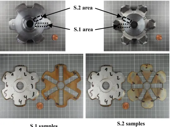
manufacturing process, the claw pole microstructure was found out to be strongly heterogeneous [12]. Thus, to address the issue of claw pole ageing, twelve specimens were extracted by wire electrical discharge machining from the plate of the rotor (Figure 1) where the gradient of grain size variation is the smallest. The choice of the cutting technique is justified by its limited impact on the magnetic properties of the cut pieces [13]. Regarding the cutting area, two sets of six-samples each are considered: S.1 samples and S.2 samples with
dimensions (35 x 10 x 1) mm3 and (27 x 10 x 1) mm3, respectively. As shown in Figure 2, the
S.1 samples are located in front of the claws and the S.2 samples were taken between the claws. The difference of dimensions between the two sets is due to the fact that between the claws, the dimensions of the area do not allow samples longer than 27 mm to be extracted. It has been shown that, with our measurement device (see 2.3), developed in [14], a variation of length from 35 mm to 27 mm have few influence on the measured magnetic characteristics.
Composition (%)
% C % Si % P % S % Mn
% weight < 0.06 % 0.07 - 0.6 % < 0.03 % 0.05 % < 0.35 %
4
Figure 1. Extraction area of samples
Figure 2.Photography of the claw pole with cutting areas of S.1 and S.2 samples
2.2. Experimental
The ageing study was carried out on both sets of samples extracted from the plate of the claw pole. After the initial characterizations, S.1-A and S.2-a samples were kept as a reference for the microstructure analysis while the others underwent isothermal ageing treatment at 180 °C for different total time periods (Table 2). In order to follow the evolution of the electric and magnetic properties throughout the ageing time, the samples were removed from the furnace, at regular time intervals of the heat treatment, and characterized at room temperature. Finally, ten samples (all samples except of S.1-E and F) were submitted to microstructural analysis and mechanical hardness test.
S.1 samples S.2 samples
S.2 area
5 Samples
Ageing time (hours)
S.1 S.2 A a Non aged B b 14 C c 21 D d 40 E e 60 F f 205
Table 2. Total ageing time periods
2.3. Characterization methods
1) Electromagnetic properties
The magnetic properties of the samples are measured with a specifically developed miniaturized SST (mini SST), as in [14], [15]. Indeed, as mentioned previously (see 2.1), because of the complex shape of the claw pole rotor and its relatively small size, the sample extraction is limited to small dimensions [14]. The characterization of the B-H magnetic hysteresis loops is based on the flux-metric method.
To measure the magnetic field H inside the sample, two Hall probes are placed next to each other along a line perpendicular to the sample surface, and as close as possible to the
sample. Thus, the magnetic fields H1 and H2 are measured at two known distances from the
sample surface and the magnetic field H at the sample surface is obtained directly by a linear extrapolation.
To measure the magnetic flux density B in the sample, a secondary coil is wound on a plastic support in which the sample is inserted. This way, all the samples are characterized using the same secondary coil to avoid a possible dispersion in the measurements due to a manual winding. Thus, the magnetic flux density B is determined accounting for the compensation of the flux in the air:
𝐵 = 1
𝑆𝑠𝑎𝑚𝑝(
1
𝑛2∫ 𝑣2(𝑡)𝑑𝑡 − 𝜇0𝐻 𝑆𝑎𝑖𝑟) (Eq 1)
where Ssamp is the cross section of the sample, 𝑛2, 𝑣2 and 𝑆𝑎𝑖𝑟 are respectively the number of
turns, the voltage and the cross-section of the secondary winding, 𝜇0 the magnetic permeability
of the vacuum and H the magnetic field estimated at the surface of the sample. For the analyses of magnetic properties, measurements are performed at an excitation frequency of 20 Hz for which the skin depth is expected to be much higher than the sample thickness for this type of material. We will also consider mainly the normal B-H curve that is obtained by collecting the
6
tips (Hp, Bp) of centered minor loops and the specific core losses that correspond to the B(H)
loop areas.
Regarding the electrical conductivity, the four-point method is employed [16]. In the configuration with a sensor having four aligned needles, a DC current is imposed between the outer pair of needles and the voltage is measured between the inner needles. However, since this method is dependent on the position of the electrical contact points and the shape of the sample, a geometry correction factor is applied as in [14], [17].
2) Microstructural and mechanical properties
To investigate the presence of precipitated particles and to evaluate the mechanical properties, the selected samples are analyzed using scanning electron microscopy (SEM) and their Vickers hardness characteristics are measured with a 3 kg load. Nevertheless, it must be pointed out that polishing (required for SEM) and hardness measurement were considered as destructive measurements since they modify the stress and strain distribution in the sample and so the magnetic properties. Hence, the hardness variation and the SEM analysis presented below were not performed on the same sample but on different samples from the same group (S.1 or S.2) which are assumed to be similar.
3. Results of thermal ageing effects on the electromagnetic properties
3.1. Thermal ageing effects on the electrical conductivity
The effect of thermal ageing on the electrical conductivity is presented in Figure 3. The characterizations were carried out as explained in Table 3. The four needles technic is no destructive which enables to measure several times the same sample during the ageing process like the sample S1.E and S1.F. According to the homogeneity of the electrical conductivity in the claw pole attested in [14] and [15], all the samples are supposed to have fairly close conductivities before ageing. Therefore, the electrical conductivity measured on the sample S.2-a is representative of those of the other samples. Regarding the uncertainty on the
measurement (±0.18 MS.m-1),calculated from the instruments precision and the measurement
limitations [18], it can be noted that the electrical conductivity before and after thermal ageing remained the same. Thus, no significant change in the electrical conductivity as a function of ageing time is observed. This is quite expected as this property depends mainly on the composition of the material which remains the same.
7 0 10 20 30 40 50 5.00 5.25 5.50 5.75 6.00 6.25 6.50 S.1 S.2 a B b D d E e F f Elec tri cal c on ductivity ( MS m -1 ) Ageing time t(h)
Effect of magnetic ageing on electrical conductivity
Figure 3. Electrical conductivity evolution as a function of thermal ageing at 180°C with ±0.18 𝑀𝑆 𝑚−1
measurement uncertainty.
Ageing time S.1 Samples S.2
Non aged a
14 hours B, E b, e
21 hours F f
27 hours D, F d, f
52 hours E, F f
Table 3. Impact of ageing on the electrical conductivity: Measurement points and characterized samples
3.2. Thermal ageing effects on the material magnetic properties
1) Magnetic losses before ageing treatment
To investigate the thermal ageing effects on the magnetic material properties, the claw pole samples were characterized before ageing at 20 Hz frequency. The measured specific losses at 1 T and 1.5 T are listed in Table 4. It appears that the S.1 and S.2 samples exhibit a clear distinct behavior before the ageing process. For example, at 1.5 T the average losses of S.2 samples are about 12 % lower than those of S.1 samples. Also, among each group of samples, a small heterogeneity is observed, with a coefficient of dispersion of 5 %. These characteristics are probably due to the manufacturing process that leads, as already observed in [12], to a heterogeneity of the microstructure (grain size, second phase particles) and residual stress levels that are known to affect the magnetic properties.
8 Samples Iron losses (W/kg) Samples Iron losses (W/kg) P1 T P1.5 T P1 T P1.5 T S.1 A 1.93 4.02 S.2 a 1.67 3.25 B 1.72 3.6 b 1.66 3.18 C 1.68 3.51 c 1.6 3.31 D 1.79 3.73 d 1.71 3.33 E 1.82 3.75 e 1.75 3.45 F 1.89 3.86 f 1.7 3.1
Table 4. Initial values of the iron losses at 1 T and 1.5 T
2) Thermal ageing effects on the material magnetic properties
Despite the initial heterogeneity noted in Table 4, the thermal ageing showed a similar behavior for all groups of samples. In fact, the final characteristics after ageing were found to be similar for all the samples. So, thereafter, for clarity of results, the effect of ageing on the hysteresis loop, the B-H normal curve and the losses will be illustrated with the data of sample S.2-e.
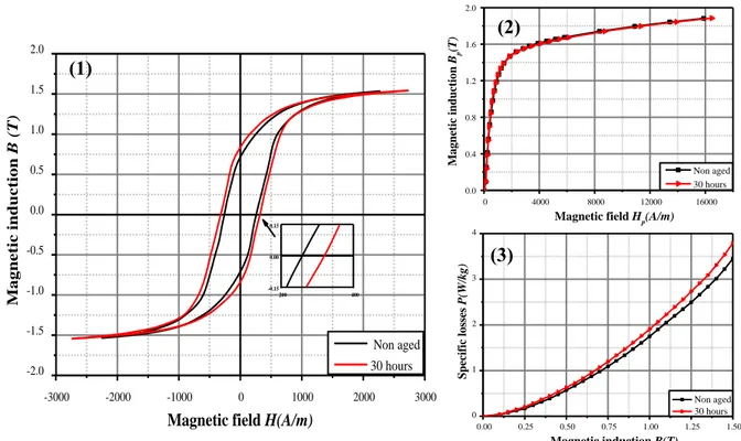
In Figure 4 (1), the measured hysteresis loops, at 20 Hz and 1.5 T induction level, are given before ageing (0 h) and after 30 hours of thermal ageing treatment at 180 °C. Comparing both hysteresis loops, an enlargement of the loop area is clearly observed leading, in the one hand, to an increase of the coercive field, which represents the magnetic field required to demagnetize the sample and, in the other hand, to an increase of the magnetic losses, as illustrated in Figure 4 (3). However, the induction level at saturation and the normal B-H curve, obtained from the tips of minor centered hysteresis loops, are slightly modified (Figure 4 (2)).
9
Figure 4. Magnetic characteristics before (0 h) and after 30 hours of thermal ageing at 180 °C at 20Hz on sample S.2-e. (1) B-H hysteresis loop (for 1.5 T magnetic induction amplitude), (2) Normal B-H curve and (3) Total magnetic losses.
3) Ageing index evolution
To further investigate the effect of ageing on the losses, these are decomposed into their
hysteresis 𝑃ℎ𝑦𝑠 and dynamic 𝑃𝑑𝑦𝑛 components such as:
𝑃𝑡𝑜𝑡 = 𝑃ℎ𝑦𝑠 + 𝑃𝑑𝑦𝑛 (Eq 2)
The hysteresis losses were calculated by extrapolating the specific energy 𝑊𝑡𝑜𝑡 = 𝑃𝑡𝑜𝑡/𝑓
to zero frequency. This has been achieved by considering measurements at four different frequencies, respectively 5 Hz, 20 Hz, 50 Hz and 100 Hz. The dynamic losses were then obtained after subtracting hysteresis losses from the total losses for each frequency. In addition, to describe and quantify the relative variation of the hysteresis losses due to the thermal ageing, the hysteresis loss ageing index (AI_hys) was calculated using (Eq 3):
𝐴𝐼_ℎ𝑦𝑠 = (𝑃ℎ𝑦𝑠)𝑎𝑓𝑡𝑒𝑟− (𝑃ℎ𝑦𝑠)before (𝑃ℎ𝑦𝑠)before
(Eq 3)
where (𝑃ℎ𝑦𝑠)before and (𝑃ℎ𝑦𝑠)𝑎𝑓𝑡𝑒𝑟 are respectively the hysteresis losses before and after thermal ageing. In Figure 5, the evolution of the index AI_hys is illustrated as a function of the
-3000 -2000 -1000 0 1000 2000 3000 -2.0 -1.5 -1.0 -0.5 0.0 0.5 1.0 1.5 2.0 Magnetic induction B (T)
Magnetic field H(A/m)
Non aged 30 hours 200 400 -0.15 0.00 0.15 0 4000 8000 12000 16000 0.0 0.4 0.8 1.2 1.6 2.0 Mag netic ind uctio n Bp (T)
Magnetic field Hp(A/m)
Non aged 30 hours 0.00 0.25 0.50 0.75 1.00 1.25 1.50 0 1 2 3 4 Sp ec ifi c los ses P(W/kg ) Magnetic induction B(T) Non aged 30 hours (3) (1) (2)
10
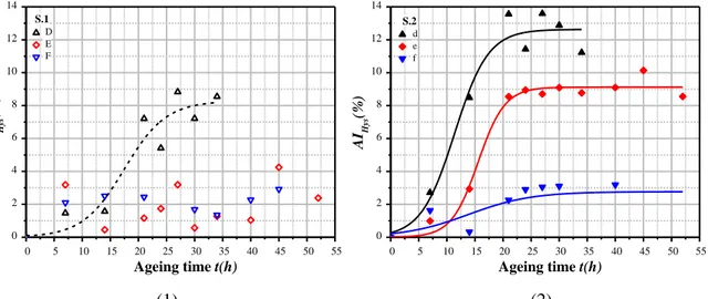
ageing time for samples which were aged for more than 30 hours (S.1- D, E, F and S.2- d, e, f) and for 1 T magnetic induction level. The hysteresis ageing index starts to considerably increase after only few hours of ageing. It reaches levels between 8 % and 14 % after about 25 hours of thermal ageing and tends to stabilize after about 30 hours of ageing. The same behavior of the hysteresis ageing index curve was observed on all the samples except for S.1- E, F and S.2-f samples whose ageing index values were lower than 5%. In particular, no significant ageing effect is observed for the samples S.1-E and F. The variability of the measurements prevents from extracting any significant tendency for the ageing index. The origin of such variability will be discussed later in section 5.3. The level reached by the ageing index varies from one sample to another; its values are reported in Table 5. Comparing the AI_hys of S.1 samples to the AI_hys of S.2 samples, it can be noted that the S.2 samples are more sensitive to ageing. These heterogeneous ageing indexes may be related to the initial microstructural characteristics of the samples that were heterogeneous. The underlying physical origins will also be discussed in section 5.3. In contrast, compared to the hysteresis losses, no significant variation was observed for the dynamic losses. For example, at magnetic induction magnitude of 1 T, the dynamic ageing index AI_dyn, calculated, as in (Eq 3) using dynamic losses at 50 Hz, does not exceed 2.5 %. Indeed, this could be explained by the fact that dynamic losses are mainly related to the electrical conductivity and we have shown experimentally that the electrical conductivity is not impacted by the magnetic ageing. Consequently, it is expected that the dynamic losses, at least the classical loss contribution [19], will not be modified by the magnetic ageing.
(1) (2)
Figure 5. Evolution of the hysteresis ageing index as a function of time for 1 T magnetic induction amplitude measurement, (1) S.1 samples and (2) S.2 samples
0 5 10 15 20 25 30 35 40 45 50 55 0 2 4 6 8 10 12 14 S.2 d e f AI Hys (%) Ageing time t(h) 0 5 10 15 20 25 30 35 40 45 50 55 0 2 4 6 8 10 12 14 S.1 D E F AI Hys (%) Ageing time t(h)
11
Ageing time (h) S.1 samples AIhys-S.1 (%) S.2 samples AIhys-S.2 (%)
14 B 5.9 b 9.7
21 C 8 c 19.9
40 D 8.8 d 13.6
60 E 4.3 e 10.1
205 F 2.9 f 3.1
* S.1-A and S.2-a were not mentioned in the table because they did not undergo the thermal ageing. They were used as reference for the microstructural analysis (SEM)
Table 5. Hysteresis ageing index highest values of S.1 and S.2 samples
4. Results of thermal ageing effects on the microstructure and mechanical hardness
4.1. Ageing effect on microstructure
To corroborate the observed ageing effect on macroscopic quantities (losses), analyses at the microstructural level are performed with a SEM (Scanning Electron Microscope) equipment. The analyses of three selected samples S.2-a, S.2-e and S.2-f, supposed to have similar initial microstructural characteristics, are performed respectively before ageing, after 60 hours and after 205 hours of thermal ageing as reported in Figure 6 and Figure 7. It is shown that before thermal ageing, only few precipitated particles (small white dots) were detected (Figure 6-(1)), while after ageing treatment the supposed carbide precipitates become more and more apparent and ever more numerous (Figure 6.-(2) and Figure 7). Moreover, according to the SEM microstructural results, it was noted that even in the samples with low AI_hys (< 5%) or apparently insensitive to ageing, as it is the case for the sample S.2-f in Figure 7, carbide precipitates are also visible. They are visually similar to those of the samples with high AI_hys (like S.2-e in Figure 6-(2)).
(1) (2)
Figure 6. Precipitate particles (1) before and (2) after 60 hours of thermal ageing at 180 °C (20 µm scale).
(Before ageing, S.2-a) (After 60 hours ageing, S.2-e)
12
Figure 7: Precipitate particles after 205 hours of ageing treatment at 180 °C (100 µm scale).
4.2. Magnetic ageing effects on the mechanical hardness
As for the magnetic properties, the presence of carbide particles impacts also the mechanical properties. Thus, the increase of precipitates was corroborated by the mechanical Vickers hardness test. Results of the test are given as a function of ageing time in Figure 8 with the hardness graphs of the S.1 and S.2 samples. First, it is noticed that the S.1 samples are globally harder than the S.2 samples. As previously explained, the difference observed between S.1 and S.2 samples in terms of hardness evolution is also probably due to the inhomogeneity of the claw pole properties induced by the manufacturing process. Second, considering the measurement confidence interval, the hardness observed for the S.2 samples does not allow to draw any conclusion. However, the hardness of the S.1 samples evolves significantly. It increases up to a maximum value (143 HV) for 21 hours of thermal ageing which coincides with the highest value of the hysteresis ageing index. After 40 hours of ageing the hardness drops to 40 HV. This behavior is discussed hereafter together with all physical observations.
100 µm
13 0 30 60 90 120 150 180 210 100 120 140 160 a b c d e f A B C D Vicker s ha rdness (HV) Ageing Time t(h) S.1 Samples S.2 Samples
Effect of magnetic ageing on the hardness
Figure 8. Vickers hardness evolution (3 kg load) as a function of ageing time for S.1 and S.2 samples
5. Discussion
5.1. Kinetic of the magnetic ageing
To clarify the observed microstructural results, it is important to consider the kinetics of carbon precipitation. In fact, during the ageing treatment, the diffusion mechanisms of the supersaturated carbon in iron α are activated. According to Fick's laws, after 21 hours of treatment at 180 °C, the distance traveled by the diffusing carbon atoms is about 5.65 µm [20]. Carbon can therefore diffuse and form precipitates of carbides, preferably in dislocations [6] which explains the intragranular precipitates observed in Figure 6 and Figure 7.
Moreover, the kinetics of ageing is linked to that of precipitation of carbides. Consequently, it can be controlled by one or more of the parameters of the precipitated carbides (volume fraction, density, texture and / or size of the particles…). Indeed, it has been reported that precipitates whose size is close to the thickness of the domain wall have the strongest pinning effect on the domain wall movements during the magnetization process [3], [21]. Furthermore, based on the theory of the inclusion of Louis Néel [3], the increase in coercivity was found out to be proportional to the volume fraction of the precipitates. Thus, the kinetics of ageing is the result of the combined effects of the size and the volume fraction of the precipitates. This could further explain the evolution of the indices AI_hyst seen in Figure 5. Three stages can be distinguished. The first presents the initiation state (first 7 hours). At this stage the carbon starts to diffuse and form precipitates. Their fraction and size are very small so their effects on the magnetic properties are limited. This step is followed by a rapid increase
14
in AI (between 7 hours and 20 hours) which corresponds to the growth phase of the precipitates. The size of the precipitates increases significantly, leading to an increase in the volume fraction. Their pining effect on the domain wall movement becomes stronger. On the other hand, the solid solution becomes depleted of carbon (reduction of supersaturated carbon). The maximum volume fraction of the precipitates is reached, and its value remains constant even in the event of coalescence. As for the size of the precipitates, once it exceeds the thickness of the domain wall, it could not cause more degradation [3], [21], [22]. This explains the trend towards the stabilization (the third stage) observed in Figure 5 after 21 hours of ageing. The same behavior was observed on semi-processed annealed electrical steel (0.034% C and 0.012% Si) in [22] with one significant difference in the ageing times compared to our study. In fact, the highest AI value was reached after more than 100 hours instead of few hours of ageing treatment. Since the chemical composition of the studied materials is quite close, this difference is principally due to the lower temperature of the ageing treatment (150 °C) considered in [22]. Nevertheless, this difference could also be attributed, in part, to the dislocation density which was reduced during the annealing treatment in [22].
5.2. The magnetic ageing and the mechanical hardness
Regarding the mechanical hardness, the evolution noted in Figure 8 is due to two phenomena which act on hardness in opposite ways. On the one hand the reduction of carbon in solid solution implies a reduction in hardness, while in the other hand, the precipitation of carbides leads to an increase in hardness. These opposite effects can explain the drop at t=40h of hardness noted on sample S.1 in Figure 8. A similar behavior was also observed by Oliveira Júnior, et al [23] with one significant difference. Indeed, Oliveira Júnior, et al noted that the ageing peaks, measured by Vickers hardness, are reached much earlier than the maximum value of the magnetic losses. This difference was explained by the fact that the size of carbides leading to a maximum effect on the movement of dislocations is much smaller than the size which anchors the magnetic domain walls movement. Yet, it could finally be concluded that even if the hardness and the magnetic ageing result from the same cause, namely the precipitation of carbides, the mechanisms impacting the magnetic properties and the mechanical hardness are not quite the same. Therefore, it is difficult to correlate the evolution of the magnetic ageing and the evolution of the mechanical hardness.
15
5.3. Analysis of the S.1 and S.2 groups ageing behavior
In order to investigate the difference in ageing kinetics between the S.1 and S.2 samples,
their average grain size was measured usingthe average grain intercept method (AGI). The
average grain size measured on ten of the twelve samples (including the S.1 and S.2 samples) turned out to be quite the same. It varies from 26 to 29 µm. Thus, it was concluded that the grain size could not be the cause behind the observed gap between S.1 and S.2 samples in terms of iron losses. However, the S.2 samples being more sensitive to magnetic ageing than the S.1 samples, one can suspect the presence of already precipitated carbides resulting from the manufacturing process. Indeed, just after the hot forging step (~1100 °C) at the beginning of the manufacturing process and the controlled cooling phase, the magnetic piece is still hot (>200°C) and is air-cooled before the next process steps. Therefore, considering the massive magnetic piece and its complex geometry, as seen in Figure 2, the region where the S.2 samples have been extracted (close to the radial edge) is more likely to cool down faster than the region where the S.1 samples have been extracted (next to the claws). Thus, given the consideration of a slower cooling rate in the region where the S.1 samples were extracted, the thermal constraints may have triggered more significantly the precipitation of carbides in S.1 samples. Accordingly, the microstructural imaging of the non-aged S.1-A sample is presented in Figure 9. It is remarkable that the white spots, representing the carbides, could exist in this sample group even before the thermal ageing treatment. Therefore, it can be concluded that the magnetic ageing of these samples started right from the manufacturing stage. Consequently, the S.1 sample losses, before the ageing treatment, are susceptible to be higher than those of the S.2 group as it was noted in Table 4.
16
To emphasize this result and make the link with the macroscopic quantities, the iron losses of the samples before and after ageing were compared. In Figure 10, the magnetic losses are given at 20 Hz frequency for the samples S.1-(D, E and F) and S.2-(d, e and f) before and after 30 hours of ageing. Indeed, above 0.8 T of magnetic induction amplitude, the loss curves before ageing show discrepancies between S.1 and S.2 sample groups. However, after the thermal ageing, the dispersion between the losses curves decreases. For example, at 1 T magnetic induction amplitude, the coefficient of variation dropped from 5% to less than 2% as illustrated in Figure 11. The loss curves show a global tendency to converge towards the same final values as observed in Figure 10-(2). This observation strengthens the hypothesis of a more advanced precipitation process in the samples of the S.1 group. Indeed, at the beginning and before the ageing treatment, in comparison to S.2 samples, the S.1 group shows higher iron losses because of a more significant presence of precipitated particles initially formed during the manufacturing process of the magnetic piece. Then, through the thermal ageing treatment applied in the present study, the precipitation process has restarted where it stopped in the S.1 samples, whereas the S.2 samples seemed to have a very limited amount of precipitations before the thermal ageing applied in the present study. Thus, the S.2 samples have exhibited a more sensitive behavior to the ageing treatment, and their iron losses have increased more significantly than those of the S.1 group. However, the compositions of both sample groups being the same, after the stabilization of the magnetic ageing effects, the iron loss curves of both sample groups finally reached the same values.
(1) (2)
Figure 10. Specific losses of S.1 and S.2 samples before (1) and after (2) thermal ageing at 20 Hz.
0.00 0.25 0.50 0.75 1.00 1.25 1.50 0.0 0.5 1.0 1.5 2.0 2.5 3.0 3.5 4.0 4.5 Specif ic l osses P(W/ kg) Magnetic induction B(T) S.1 S.2 D d E e F f
Specific losses at 20 Hz - Before aging
S.1 S.2 0.00 0.25 0.50 0.75 1.00 1.25 1.50 0.0 0.5 1.0 1.5 2.0 2.5 3.0 3.5 4.0 4.5 Specific losses P(W/kg) Magnetic induction B(T) S.1 S.2 D d E e F f
17 0.8 1.0 1.2 1.4 1.6 0 2 4 6 8 CV (%) Bp(T) Before ageing After ageing Comparaison between the coefficients of variation of losses
Figure 11. Evolution of the coefficient of variation 𝐶𝑣 of the losses (all samples considered) before and after
ageing (with 𝐶𝑣the ratio of the loss standard deviation on the mean losses value)
6. Conclusion
The present work has investigated the magnetic ageing of a steel grade used for the manufacturing of massive magnetic parts of claw pole synchronous machine. The composition of the material as well as the operating conditions of the electrical machine (about 180 °C for some operating points) strongly suggest that magnetic ageing should occur. The obtained results showed a clear evolution of the magnetic properties during the proposed thermal ageing process. Indeed, even if the normal B-H curve is not significantly modified after the ageing process, the losses increase significantly, up to 14 % for some samples. These observations are supported by microstructural analyses showing an increase of carbides precipitates inside the grains. This mechanism explains the loss increase, especially the hysteresis loss contribution, as these microstructural precipitates act as pinning sites for magnetic domain walls during the magnetization process. Moreover, due to the manufacturing process of the investigated magnetic part (the claw pole rotor being obtained from hot and cold forging processes without annealing), heterogeneous properties were observed from one sample to another before the ageing process. The samples, extracted from two different locations in the magnetic piece, exhibit different evolutions of the ageing index. The possibility of a pre-existing carbide precipitations during the manufacturing process is suspected. Also, the tendency of all samples to have the same magnetic losses at the end of the ageing process supported this hypothesis. The maximum effects of the thermal ageing, at the same temperature of operation of the device, on magnetic losses were achieved after only 21 hours of thermal ageing. Therefore, magnetic ageing may occur rapidly during the first hours of operation of the energy conversion device. In the case of the claw pole alternator application, in the majority of the core, the plates and
18
claws are subjected to a DC excitation. The major losses in the rotor are due to dynamic ones induced by the flux pulsations at the surface of the claws due to the rotor movement in front of the stators teeth. So, the influence of ageing on the losses may be finally negligible. Nevertheless, for other applications in which the magnetic core is exposed to AC excitation, the influence of ageing on the magnetic properties, especially the losses, should be taken into consideration in the design and performance simulation of the energy conversion device. Acknowledgements
The authors would like to thank Jean-Bernard Vogt from UMET- University of Lille for access to microstructural and mechanical measurement facilities.
References
[1] S. Brisset, M. Hecquet, and P. Brochet, “Thermal modelling of a car alternator with claw poles using 2D finite element software,” COMPEL - Int. J. Comput. Math. Electr.
Electron. Eng., vol. 20, no. 1, pp. 205–215, Jan. 2001, doi:
10.1108/03321640110359930.
[2] K. Jenkins and M. Lindenmo, “Precipitates in electrical steels,” J. Magn. Magn. Mater., vol. 320, no. 20, pp. 2423–2429, Oct. 2008, doi: 10.1016/j.jmmm.2008.03.062.
[3] M. F. de Campos, M. Emura, and F. J. G. Landgraf, “Consequences of magnetic aging for iron losses in electrical steels,” J. Magn. Magn. Mater., vol. 304, no. 2, pp. e593– e595, Sep. 2006, doi: 10.1016/j.jmmm.2006.02.185.
[4] N. M. Benenson and Z. I. Popova, “Kinetics of magnetic aging of low-carbon electrical steel,” Met. Sci. Heat Treat., vol. 10, no. 4, pp. 278–283, Apr. 1968, doi:
10.1007/BF00653109.
[5] G. M. Michal and J. A. Slane, “The kinetics of carbide precipitation in silicon-aluminum steels,” Metall. Trans. A, vol. 17, no. 8, pp. 1287–1294, Aug. 1986, doi:
10.1007/BF02650109.
[6] S. K. Ray and O. N. Mohanty, “TEM Investigation of Carbide Precipitation in Low Carbon Steels Containing Silicon,” Trans. Jpn. Inst. Met., vol. 24, no. 2, pp. 81–87, 1983, doi: 10.2320/matertrans1960.24.81.
[7] K. M. Marra, F. J. G. Landgraf, and V. T. Buono, “Magnetic losses evolution of a semi-processed steel during forced aging treatments,” J. Magn. Magn. Mater., vol. 320, no. 20, pp. e631–e634, Oct. 2008, doi: 10.1016/j.jmmm.2008.04.023.
[8] S. K. Ray and O. N. Mohanty, “Magnetic ageing characteristics of low silicon electrical steels,” J. Magn. Magn. Mater., vol. 28, no. 1, pp. 44–50, Jul. 1982, doi: 10.1016/0304-8853(82)90027-0.
[9] W.-M. Mao, P. Yang, and C.-R. Li, “Possible influence of sulfur content on magnetic aging behaviors of non-oriented electrical steels,” Front. Mater. Sci., vol. 7, no. 4, pp. 413–416, Dec. 2013, doi: 10.1007/s11706-013-0219-3.
[10] J. M. Pardal, S. S. M. Tavares, M. P. Cindra Fonseca, M. R. da Silva, J. M. Neto, and H. F. G. Abreu, “Influence of temperature and aging time on hardness and magnetic
properties of the maraging steel grade 300,” J. Mater. Sci., vol. 42, no. 7, pp. 2276– 2281, Mar. 2007, doi: 10.1007/s10853-006-1317-8.
19
[11] W. C. Leslie and D. W. Stevens, “The magnetic aging of low-carbon steels and silicon irons,” Trans ASM, vol. 57, pp. 261–283, 1964.
[12] M. Borsenberger, “Contribution à l’identification de l’interaction paramètres procédés – propriétés d’emploi des produits : Application au forgeage et aux propriétés
électromagnétiques d’une roue polaire d’alternateur,” thesis, Paris, ENSAM, 2018. [13] H. Naumoski, B. Riedmüller, A. Minkow, and U. Herr, “Investigation of the influence
of different cutting procedures on the global and local magnetic properties of non-oriented electrical steel,” J. Magn. Magn. Mater., vol. 392, pp. 126–133, Oct. 2015, doi: 10.1016/j.jmmm.2015.05.031.
[14] M. Jamil, A. Benabou, S. Clénet, L. Arbenz, and J.-C. Mipo, “Development and validation of an electrical and magnetic characterization device for massive
parallelepiped specimen,” Int. J. Appl. Electromagn. Mech., pp. S1–S8, Jun. 2019, doi: 10.3233/JAE-191491.
[15] M. Toto Jamil, A. Benabou, S. Clénet, S. Shihab, L. Le Bellu Arbenz, and J.-C. Mipo, “Magneto-thermal characterization of bulk forged magnetic steel used in claw pole machine,” J. Magn. Magn. Mater., vol. 502, p. 166526, May 2020, doi:
10.1016/j.jmmm.2020.166526.
[16] L. Arbenz, A. Benabou, S. Clenet, J. C. MIPO, and P. Faverolle, “Characterization of the local Electrical Properties of Electrical Machine Parts with non-Trivial Geometry,”
Int. J. Appl. Electromagn. Mech., vol. 48, no. 2 & 3, pp. 201–206, Jun. 2015, doi:
10.3233/JAE-151988.
[17] F. M. Smits, “Measurement of Sheet Resistivities with the Four-Point Probe,” Bell Syst.
Tech. J., vol. 37, no. 3, pp. 711–718, May 1958, doi:
10.1002/j.1538-7305.1958.tb03883.x.
[18] JCGM, “Evaluation of measurement data — Guide to the expression of uncertainty in measurement.” BIPM, 2008.
[19] G. Bertotti, “General properties of power losses in soft ferromagnetic materials,” IEEE
Trans. Magn., vol. 24, no. 1, pp. 621–630, Jan. 1988, doi: 10.1109/20.43994.
[20] G. Murry, Aide-mémoire - Métallurgie Métaux, Alliages, Propriétés. Paris: Dunod. [21] J. Wang, Q. Ren, Y. Luo, and L. Zhang, “Effect of non-metallic precipitates and grain
size on core loss of non-oriented electrical silicon steels,” J. Magn. Magn. Mater., vol. 451, pp. 454–462, Apr. 2018, doi: 10.1016/j.jmmm.2017.11.072.
[22] A. A. de Almeida and F. J. G. Landgraf, “Magnetic Aging, Anomalous and Hysteresis Losses,” Mater. Res., vol. 22, no. 3, p. e20180506, 2019, doi: 10.1590/1980-5373-mr-2018-0506.
[23] J. R. de Oliveira Júnior et al., “Kinetics of Magnetic Ageing of 2%Si Non-oriented Grain Electrical Steel,” Mater. Res., vol. 21, no. 1, 2018, doi: 10.1590/1980-5373-mr-2017-0575.