HAL Id: inserm-00663765
https://www.hal.inserm.fr/inserm-00663765
Submitted on 27 Jan 2012
HAL is a multi-disciplinary open access
archive for the deposit and dissemination of
sci-entific research documents, whether they are
pub-lished or not. The documents may come from
teaching and research institutions in France or
abroad, or from public or private research centers.
L’archive ouverte pluridisciplinaire HAL, est
destinée au dépôt et à la diffusion de documents
scientifiques de niveau recherche, publiés ou non,
émanant des établissements d’enseignement et de
recherche français ou étrangers, des laboratoires
publics ou privés.
Large-scale prediction of protein-protein interactions
from structures
Martial Hue, Michael Riffle, Jean-Philippe Vert, William Noble
To cite this version:
Martial Hue, Michael Riffle, Jean-Philippe Vert, William Noble. Large-scale prediction of
protein-protein interactions from structures. BMC Bioinformatics, BioMed Central, 2010, 11 (1), pp.144.
�10.1186/1471-2105-11-144�. �inserm-00663765�
R E S E A R C H A R T I C L E
Open Access
Large-scale prediction of protein-protein
interactions from structures
Martial Hue
1,2,3, Michael Riffle
4,5, Jean-Philippe Vert
1,2,3, William S Noble
5,6*Abstract
Background: The prediction of protein-protein interactions is an important step toward the elucidation of protein functions and the understanding of the molecular mechanisms inside the cell. While experimental methods for identifying these interactions remain costly and often noisy, the increasing quantity of solved 3D protein structures suggests that in silico methods to predict interactions between two protein structures will play an increasingly important role in screening candidate interacting pairs. Approaches using the knowledge of the structure are presumably more accurate than those based on sequence only. Approaches based on docking protein structures solve a variant of this problem, but these methods remain very computationally intensive and will not scale in the near future to the detection of interactions at the level of an interactome, involving millions of candidate pairs of proteins.
Results: Here, we describe a computational method to predict efficiently in silico whether two protein structures interact. This yes/no question is presumably easier to answer than the standard protein docking question, “How do these two protein structures interact?” Our approach is to discriminate between interacting and non-interacting protein pairs using a statistical pattern recognition method known as a support vector machine (SVM). We demonstrate that our structure-based method performs well on this task and scales well to the size of an interactome.
Conclusions: The use of structure information for the prediction of protein interaction yields significantly better performance than other sequence-based methods. Among structure-based classifiers, the SVM algorithm, combined with the metric learning pairwise kernel and the MAMMOTH kernel, performs best in our experiments.
Background
The knowledge of the interactions among proteins is essential to understanding the molecular mechanisms inside the cell. However, the experimental measurement of protein-protein interactions by two main procedures– the yeast two-hybrid system and mass spectrometry combined with tandem affinity purification–suffers from a high false positive rate, as evidenced by the small intersection between several independently generated interaction data sets [1]. Recent years have seen much progress in understanding of the false positive predic-tions [2]. The limitapredic-tions of current experimental meth-ods therefore highlight the need for in silico interaction predictions.
The elucidation of an increasing number of protein 3D structures is likely to continue at a fast pace as a result of several large-scale initiatives. These structures provide both an opportunity and a challenge for in silico prediction methods. The opportunity is that if in silico methods are able to predict whether two given 3D structures interact, then these methods may be applied to predict interactions among the large amount of pro-teins with known or inferred 3D structure. The chal-lenge is that these methods need to be computationally fast to scale to the prediction of interactions among mil-lions or more candidate pairs of structures. Unfortu-nately, the current methods of choice to predict interactions are mostly based on the idea of docking, which is very computationally intensive and therefore unlikely to be able to scale to large interactomes in the near future. See [3] for a review of the issues related to the prediction of interaction using protein-protein
* Correspondence: [email protected]
5Department of Genome Sciences University of Washington, Seattle, WA,
USA
© 2010 Hue et al; licensee BioMed Central Ltd. This is an Open Access article distributed under the terms of the Creative Commons Attribution License (http://creativecommons.org/licenses/by/2.0), which permits unrestricted use, distribution, and reproduction in any medium, provided the original work is properly cited.
docking, and [4] for a review of the problem of predict-ing interactions uspredict-ing structural information.
In this study, we are interested in developing methods to predict whether two proteins interact. We aim to develop a method that will scale to the analysis of whole proteomes in order to identify candidate protein pairs for further analysis by more computationally expensive procedures. Docking not only attempts to answer the question of whether two proteins interact, but also how they interact. Our strategy is to develop methods that predict less information than docking, by focusing only on the first question, trading this decrease in the rich-ness of prediction for an increase in computational effi-ciency. Note that, in general, the problem of predicting protein-protein interactions is complicated by multi-domain proteins. For simplicity in this work, we will therefore focus on predicting whether a given pair of protein domains interacts. We aim at answering the question: “Given two domain structures, do they inter-act?” Our strategy to solve this problem is to formalize it as a binary classification problem, and to train a dis-criminative classifier to answer the question of whether or not a pair of domain structures interact, using as training data examples of known interacting and non-interacting pairs.
This idea is related to previous applications of machine learning techniques to predict protein-protein interactions from a variety of data types, including noisy interaction networks, localization information, sequence and expression data. These techniques include Bayesian networks [5], support vector machines [6-9], decision trees [10,11] and random forests [12]. Shoemaker et al. [13] review the approaches for predicting protein-pro-tein interactions, and [14] compare existing approaches on a common data set. However, to our knowledge, machine learning methods have not previously been applied to the prediction of protein-protein interactions from protein structures.
¿From a technical point of view, we face two issues to implement this strategy. First, we must be able to manipulate protein 3D structures in the context of a machine learning algorithm. For this we borrow an idea from [15], who proposed using a classical measure of structural similarity to implicitly embed 3D structures in a vector space. Second, once we represent each 3D structure as a vector, we must be able to learn a classifi-cation function over pairs of vectors. For this we test different strategies that have been proposed recently to solve this issue with kernel methods such as SVMs [9,16]. Combining these two ideas, we propose two learning algorithms that can be combined with two pos-sible representations of pairs of 3D structures to predict interactions, resulting in four methods. In order to assess the benefits of using 3D structure information for
this purpose, rather than using sequence information only, we additionally test the same four methods starting from a measure of primary sequence similarity, instead of 3D structure similarity.
In order to test these methods, we construct three benchmarks from known interactions between proteins of known or inferred structures. We compare the per-formance of the different methods in a cross-validation procedure. As a baseline, we compare to similar meth-ods that exploit only amino acid sequences. These experiments suggest that the metric learning pairwise kernel [16], coupled with a support vector machine clas-sifier, yields the best performance.
Methods
Our approach to predict whether two proteins interact is to frame the question as a supervised learning pro-blem. Based on examples of interacting pairs and non-interacting pairs, we train a binary classifier to predict the class ("interacting” or “non-interacting”) of a pair of protein structures. In this study, we compare eight dif-ferent classification methods, corresponding to all com-binations with respect to three binary choices: (1) two classification algorithms, (2) two vector encodings of proteins, based on structure or sequence, respectively, and (3) two different methods for computing the simila-rities among pairs of vectors. In the following, we first describe the two classification algorithms, the two simi-larity functions, and then the two methods for comput-ing pairwise similarities.
Classification algorithms Nearest neighbor
As a simple baseline algorithm, we use the nearest neighbor algorithm (NN). Given a training set of n points x1,...,xn labeled y1,...,yn in {-1, +1}, NN assigns
to a test point x the class label of the majority among the k nearest training set points. In our case, rather than a simple binary label, we would like the algorithm to return a real-valued discriminant score in order to be able to rank the prediction by confi-dence. For this purpose, we use the difference in the sum of the distances to the k nearest positive and the sum of distances to the k nearest negative training set examples: fNN x d x xi d x xi x x xi k x i k ( ) ( , ) ( , ) ( ) ( )
(1)The predicted class label is simply the sign of this dis-criminant. k
(resp.
k
) denotes the set of k nearest
negative (resp. positive) neighbors. The value of k is selected via cross-validation, as described in the Results section.
Hue et al. BMC Bioinformatics 2010, 11:144 http://www.biomedcentral.com/1471-2105/11/144
NN is perhaps the simplest example of a broad class of algorithms known collectively as kernel methods [17]. An algorithm is a kernel method if and only if it can be formulated such that every occurrence of a data vector x occurs inside of a scalar product operation. In this case, every instance of the scalar product operation can be replaced by a generalized notion of similarity, called the kernel function. Formally, a kernel function is a sym-metric positive semidefinite function, which provably corresponds to the scalar product operation in some vector space. Using a kernel function in place of the sca-lar product operation implicitly maps the given data set into a possibly high-dimensional space (called the fea-ture space) that may be non-linearly related to the input spacein which the data resides.
To “kernelize” the nearest neighbor algorithm, we simply note that the Euclidean distance can be stated entirely in terms of scalar product operations:
d x x x x x x x x x x ( , ) ( ) ( ) ( ), ( ) ( ), ( ) ( ), ( ) 2 ..
In terms of the kernel function K( x , x) = 〈;F( x ), F (x)〉;, therefore,
d x x( , ) K x x( , ) 2K x x( , ) K x x( , ). (2) The kernel NN algorithm simply substitutes Equation (2) into Equation (1). Below, we define three different kernel functions and use each of them to create a NN classifier for predicting protein-protein interactions.
Support vector machine
Functionally, the support vector machine (SVM) [18] is similar to the nearest neighbor algorithm. Both are supervised classification algorithms, and both are kernel methods. However, unlike the nearest neighbor approach, the SVM algorithm attempts to find a hyper-plane that optimally separates examples from the two given classes. The SVM algorithm is appealing due to its mathematical properties and its successful application to a wide variety of classification problems in computa-tional biology [19].
Training an SVM involves solving a convex quadratic program, which can be formulated as follows:
min , , w b i i n w C 2 1
subject to the constraints
i 1 ,n yi(w, ( ) xi b) 1 i.
The solution to this optimization is a hyperplane hw,b = {x: 〈w, F(x)〉 + b = 0}, and the classification
procedure for a novel test point x involves computing which side of the hyperplane the point lies on. The SVM discriminant is the signed distance to the hyperplane:
fSVM( )x w, ( )x b.
Like NN, the SVM can also be subjected to the “ker-nel trick,” the details of which we omit here for brevity. The SVM depends on a user-specified regularization term, C ≥ 0, which prevents overfitting to noise in the data or noise in the labels. In the case of unbalanced data, we apply this regularization asymmetrically to positive and negative examples, as follows:
min , , : : w b i i y i i y w C C i i 2 0 0
(3)The values of C+ and C-are selected via
cross-valida-tion, as described in the Results section.
Kernel on proteins
In order to use a NN or SVM algorithm to predict interactions between proteins, we must define a kernel between the objects for which predictions are to be made, namely, pairs of proteins. In this section, we describe two kernels that are defined with respect to individual proteins. In the next section, we describe methods for generalizing from these single-protein ker-nels to kerker-nels on protein pairs.
A kernel on protein structures
A natural place to begin, when considering comparisons among protein structures, is with structural alignment algorithms such as CE [20], DALI [21] and MAM-MOTH [22]. These algorithms create an alignment between two proteins and then compute a score that reflects the alignment’s quality. In this work, we use MAMMOTH [22], which is efficient and produces high quality alignments. We treat the output of MAMMOTH as an arbitrary score, denoted s(p, q).
Unfortunately, the alignment quality score returned by MAMMOTH cannot be used as a kernel function directly, because the score is not positive semidefinite (i.e., for a given set of protein structures, an all-versus-all matrix of MAMMOTH scores will usually have some negative eigenvalues). To define a MAMMOTH kernel on protein structures, we therefore subtract the negative portion of the eigenvalue spectrum to convert the score to a kernel. Namely, if M is the MAMMOTH similarity matrix, then Mis symmetric with singular value decomposition
MU DV
where D is a diagonal matrix diag (l1,...,ln). The
K U( ) .D V
with Ψ(D) = diag(ψ(l1),...,ψ(ln)), and ψ(l) = 1 + l if
l> 0, and 0 otherwise.
In practice, we normalize this kernel by projecting onto the unit sphere, via the transformation
ˆ ( , ) ( , ) / ( , ) ( , ).
K p q K p q K p p K q q (4)
A related MAMMOTH kernel has previously been shown to yield good performance in classifying proteins into SCOP categories or by GO terms [15]. It uses ψ(l) = l2.
A kernel on protein sequences
We compare our methods based on structures to corre-sponding sequence-based methods, as a baseline. We borrow an idea of a kernel on sequences from [23]. The mismatch kernel induces a distance measure between protein sequences. A protein sequence a is mapped to a feature vector
k m, ( ) { ( )} k
where is the alphabet of 20 amino acids. The neighbourhood k,m(a) of a k-mer a is the set of
k-mers that differs in at most m positions. The feature vector encodes the all the k-mers in the neighborhood:
( ) , ( ) 1 0 if otherwise. k m
Thus, the mismatch kernel between two protein sequences x and y is
Kk m, ( , )x y k m, ( ),x k m, ( )y
In our experiments, we set k = 6 and m = 1.
Kernels for pairs of objects
This section describes techniques for deriving, from the single-protein kernels described in the previous Section, a pairwise kernel function K((p1, p2), (q1, q2)) that
quan-tifies the degree of similarity between two protein pairs. In particular, we present two pairwise kernels: the ten-sor product pairwise kernel (TPPK) and the metric learning pairwise kernel (MLPK).
Tensor product pairwise kernel
The tensor product pairwise kernel (TPPK) is a general method for building a kernel for pairs of objects from any kernel K for objects. This kernel has been used suc-cessfully for predicting protein-protein interactions from sequence [24] and from a combination of sequence, annotation, network topology and interolog features [9].
The TPPK considers two pairs of proteins to be simi-lar to one another when each protein from one pair is similar to one protein of the other pair. For example, if p1 is similar to q1 and p2 is similar to q2, then we can
say that the pairs (p1, p2) and (q1, q2) are similar to one
another. We can translate these intuitions into the fol-lowing pairwise kernel:
KTPPK(( ,p p1 2),( ,q q1 2))K p q K p q( ,1 1) ( 2, 2)K p q K p q( ,1 2) ( 2, 1), (5)
where K is the kernel on proteins. The feature space for TPPK is the tensor product of the feature spaces of each member of the pair, so if M is the dimensionality of the feature space, then the dimensionality of the fea-ture space of the tensor product is M2.
Note that, as formulated in Equation (5), the TPPK has the counter-intuitive property that two protein pairs can be considered similar if the underlying protein pairs are strongly dissimilar. This is because the base kernel function K can return negative values which, when mul-tiplied together, yield a positive value for KTPPK. To
avoid this artifact, we add 1 to the base kernel function, so that the kernel values lie in the range [0, 2]. This operation preserves a valid kernel, because the matrix of all 1’s is positive definite, and the sum of two positive definite matrices is a positive definite matrix. Without this “add 1” correction, the TPPK results are signifi-cantly worse (data not shown).
Metric learning pairwise kernel
Similar to TPPK, the metric learning pairwise kernel (MLPK) is a method for building a kernel for pairs of objects based on a kernel K for objects [16]. However, MLPK represents a pair of objects as the difference between its members. In this case, a pair (p1, p2) of
objects is represented in the feature space by the differ-ence p1 - p2, squared (by the tensor product operation)
to make it invariant with respect to the order of the proteins. The MLPK was presented in [16] as a way to learn a new metric between individual objects (3D struc-tures in our case). The corresponding MLPK between the pair (p1, p2) and (q1, q2) is
KMLPK(( ,p p1 2),( ,q q1 2))[ ( ,K p q1 1)K p q(2, 2)K p q(2, 1)K p q( ,1 2))] .2 (6)
For consistency with the TPPK, we add 1 to each entry of K.
Data
We built a benchmark of interacting pairs of protein structures, based on the Database of Interacting Proteins (DIP) [25] downloaded on January 26, 2009. The com-plete database contains 88,618 interactions among 27,496 proteins. From these interactions, we selected two subsets. The first is the “Core” dataset, which
Hue et al. BMC Bioinformatics 2010, 11:144 http://www.biomedcentral.com/1471-2105/11/144
consists of a set of 4,553 interactions among 2,423 S. cerevisiae proteins. These interactions are considered reliable based on expression data and the presence of paralogous interacting protein pairs [1]. The second data set, “small-scale,” consists of interactions that were verified by small-scale experimental methods, using techniques that reliably indicate direct physical interac-tion of proteins. These methods include immunoprecipi-tation, cross-linking, in vitro binding, X-ray diffraction, competition binding, electron microscopy and X-ray crystallography, for a total of 2,622 interactions among 2,408 proteins. For each of the two sets of interactions, we collected a set of protein structures using the follow-ing protocol:
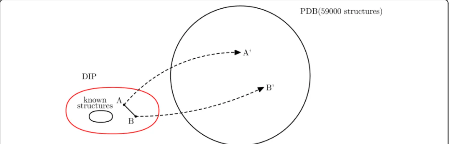
1. We use PSI-BLAST to search for homologous proteins with known structures, as shown in Figure 1. For each protein in a given DIP data set, we search the domains of the PDB using PSI-BLAST for a maximum of 5 iterations [26]. For each protein, we identify at most one homolog that is longer than 50 amino acids and achieves an E-value less than 10 -20.
2. All of our methods require negative examples for training. To avoid biasing the selection of negatives, we choose non-interacting protein pairs at random from a non-redundant subset of the PDB [27]. This subset consists of 8,261 structures, selected using the PISCES Database with a percent identify cutoff of 70% and a resolution of 2.0 Å or better (downloaded on March 2nd, 2009). At this stage, we select five times as many negative pairs as positive pairs. 3. We filter the combined collection of positive and negative pairs to remove redundant pairs. For each data set, we cluster the protein sequences using BLASTClust [26] with a threshold of 40% sequence identity. We search for cases in which pairs of
proteins link the same two clusters. If all pairs are negative, then we remove all except one randomly selected pair. If one pair is positive and others are negative, then we remove the negative pairs. If two or more pairs are positive, then we remove all the pairs except the positive one that has the minimal number of (positive) neighbors.
4. Finally, we remove all negative pairs that involve a protein shorter than 50 amino acids and then ran-domly downsample the remaining negative pairs so that the ratio of negative to positive pairs is 3:1. This procedure generated two different data sets. The “core” data set contains 6,175 proteins, with 1,581 inter-acting pairs involving 824 proteins and 4,743 non-inter-acting pairs. The “small-scale” set contains 6,187 proteins, with 1,392 interacting pairs involving 1,175 proteins and 4,176 non-interacting pairs. We also build a subset of the “core”, called “core-subset,” that contains the same number of interacting pairs as the small-scale. Note that we also generated three additional “core” and three additional “small-scale” data sets, using homology thresholds of 10-20and 10-5and redundancy thresholds
of 40% and 90%. The sizes and cross-validation results from those data sets are summarized in the Additional file 1.
All data sets used in this study are available at http:// noble.gs.washington.edu/proj/pips.
Results
For each of the eight classifiers, we performed 5-fold cross-validation, repeated three times (3×5cv). During each SVM training, an internal 5-fold cross-validation was performed to select two regularization parameters using grid search. We selected the regularization para-meter associated with interacting pairs (C+) from {10-8,
10-7,..., 108}, and we selected the ratio C+/C-from {3, 10,
Figure 1Benchmark generation. For each interacting pair of proteins with unknown structure, we use a proxy pair of homologs with known structure.
100}. The parameter k of NN was selected from {1, 2, 3, 5, 10, 15}.
In each testing phase of the cross-validation, the pro-portion of negative examples with respect to positive examples is equal to r = 3. In a more realistic setting, this ratio would be much higher. Therefore, we extrapo-late from the measured precision p to estimate the pre-cision of each classifier in the case where all negative examples were considered in the benchmark. If v is the number of proteins, and e is the number of interacting pairs, then the ratio of negative to positive examples is r’ = (v * (v - 1)/2 - e)/e. The estimated precision thus becomes p/(p + r’/r * (1 - p)).
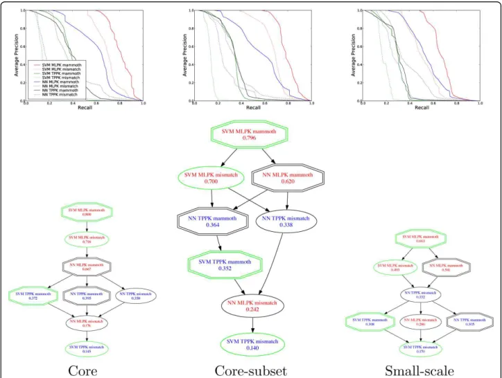
Figure 2 shows, in the top row, precision-recall curves comparing the performance of the eight different classi-fiers across the 15 splits, incorporating the
post-processing of precisions described in the previous para-graph. We use precision-recall curves rather than recei-ver operating characteristic curves because the latter removes the effect of the skewed positive-to-negative ratio [28]. In Figure 2, the performance of a random classifier would be represented by a horizontal line cor-responding to a constant precision, the ratio of the posi-tive to negaposi-tive class over the whole test set (approximately y = 0.001). Except at high recall, all of the methods perform much better than chance.
To evaluate the statistical significance of the differ-ences in performance observed in the top row of Figure 2, we performed Wilcoxon signed-rank tests on the area under the precision-recall curve across the 15 splits of the 3×5cv of the four data sets. The bottom row of panels in Figure 2 shows the results of this test. In the
Figure 2Comparison of methods for predicting protein-protein interactions. The top three panels plot the average precision (TP/(TP+FP)) as a function of recall (TP/(TP+FN)) for the core, core subset and small-scale benchmarks. Each precision is averaged across the 15 splits of 3×5cv, and estimated for test sets for which the negative examples are not downsampled. In the lower three panels, an edge from method A to B indicates that method A outperforms method B at p > 0.5 according to a Wilcoxon signed rank test applied to the area under the precision-recall curve, computed separately for each of the 15 splits of 3×5cv. Redundant edges have been removed for clarity; i.e., the figure shows the transitive reduction of the full graph.
Hue et al. BMC Bioinformatics 2010, 11:144 http://www.biomedcentral.com/1471-2105/11/144
graph, an edge from method A to B indicates that method A outperforms method B according to the Wil-coxon test with p < 0.05. Redundant edges have been removed for clarity; i.e., the figure shows the transitive reduction of the full graph.
The signed-rank results show two expected trends across the three benchmarks. First, in general, structure-based methods perform better than the corresponding sequence-based methods. In particular, classifiers that use a MAMMOTH kernel outperform the correspond-ing mismatch kernel method in 9 cases out of 12, and never perform worse.
Second, SVM-based methods generally perform better than nearest neighbors methods, although this trend is not as consistent (6 wins, 2 draws and 4 losses). The relative performance of the SVM and NN classifiers seems to depend in part upon which pairwise transfor-mation is employed. In conjunction with the MLPK transformation, the SVM outperforms the NN in all six cases. In contrast, when the TPPK transformation is employed, NN performs better than the SVM in four cases, and ties in the remaining two. Although the rela-tive performance of the MLPK and TPPK transforma-tions is difficult to explain [16], one may speculate that the TPPK definition (5) results in a more natural mea-sure of similarity between pairs than the MLPK one (6); hence, TPPK is likely to behave better with a NN classi-fier. On the other hand, the MLPK transform can be justified from the point of view of metric learning when used in combination with an SVM [16], but MLPK remains an obscure measure of similarity between pairs, which may therefore not be optimally used by a NN classifier.
Finally, with respect to MLPK versus TPPK, the MLPK transformation performs best overall. In 9 out of 12 cases, the MLPK method outperforms the corre-sponding TPPK method. The only three exceptions are NN classifiers using sequence kernels, which are rela-tively poorly performing methods overall. Overall, our experiments suggest that, for the prediction of protein-protein interactions from structure, the MLPK SVM combined with MAMMOTH is the best method among the eight that we considered. This method performs best on all three benchmarks.
Having selected the best performing method, we used an SVM to predict novel interactions among all pairs of proteins in a non-redundant subset of the PDB. We used the PISCES Database with a percent identify cutoff of 90% and a resolution of 2.5 Å or better (downloaded on January 26, 2009), eliminating proteins shorter than 60 amino acids and longer than 300 amino acids. This set contains 9,574 structures. Prior to the SVM analysis, we eliminated pairs that are similar to any member of the training set. Specifically, for a candidate pair (p1, p2),
we define the distance to a training set pair (q1, q2) as D p p(( ,1 2),( ,q q1 2))min(max( ( ,E p q1 1), (E p q2, 2)), max( ( ,E p q1 2),, (E p q2,1))),
where E(p, q) is the BLAST E-value assigned to query p against target q. We only consider candidate pairs for which the minimum distance to any member of the train-ing set exceeds an E-value of 0.01. This filtertrain-ing reduces the complete set from 45,835,525 to 45,676,254 pairs. We applied to each of these pairs the SVM MLPK MAM-MOTH method, trained on 90% of the small-scale DIP benchmark, and we used the held-out 10% of the data to convert the SVM discriminants to probabilities [29].
At a threshold of 99%, the SVM predicts 4,826 novel interactions; at 90%, the SVM predicts 108,491 pairs. The latter set is publicly available via the Yeast Resource Center Public Data Repository http://yeastrc.org/pdr[30].
Discussion
We presented eight machine learning methods for large-scale prediction of interactions between pairs of protein structures. The methods use either a NN or a SVM clas-sifier, coupled with two kernels on protein sequences or structures, coupled with two methods for representing similarities between pairs of protein. In our cross-valida-tion experiment, we observed–not surprisingly–that structure-based methods are generally more accurate than the methods based on sequence. Among structure-based classifiers, the SVM with an MLPK kernel per-forms best.
The classifiers described here only use structural or sequence information about the proteins. Further improvements in prediction accuracy could probably be obtained by taking into account other information such as expression profiles or sub-cellular localization. The integration of such heterogeneous data could for exam-ple be carried out by creating different kernels from each type of information, and merging the information by forming a linear combination of all individual kernels [9,31].
One shortcoming of our approach is that each protein interaction is predicted independently. We believe that taking into account the topology of the whole interac-tion graph might improve the accuracy of the predic-tions. However, generalizing binary prediction to more complex prediction, such as graph prediction, remains a challenging issue and an active research topic in the machine learning community.
In the course of this study we generated eight bench-marks that we make publicly available and which can be used to assess the performance of other methods for the automated prediction of interaction between protein structures. The benchmark generation depends on two parameters: the homology threshold, to be input to
PSI-BLAST to find a proxy pair, and the redundancy thresh-old to be input to BLASTClust. For each of the bench-marks, we set the values of the homology threshold to 10-5, and 10-20, and the values of the redundancy
thresh-olds to 40 and 90, leading to four datasets for each benchmark. Here, we reported the cross-validation results of only one dataset; however, the conclusions do not change when we consider the cross-validation experiments on the other benchmark data sets.
Finally, as pointed out in the introduction, the main motivation behind this work is to perform a large-scale screening of pairs of proteins likely to interact, before validating the prediction by more expensive computa-tional methods such as docking, or experimental meth-ods for pairs of particular interest. This will be the subject of future work.
Conclusions
The eight presented machine learning methods based on kernel methods to predict the binary interaction between protein structures were evaluated on a data set of reliable interations. We draw three main conclusions from our experiments. First, using structure we can more accurately predict interactions than using sequence alone. Second, SVM methods compare favor-ably against the methods based on the nearest neighbor classifier. Third, the best choice of pairwise metric asso-ciated with the predictor is MLPK rather than TPPK.
Additional file 1: Cross-validation results on additional Core and Small-scale datasets. The file contains the size and cross-validation results of eight datasets, including three additional Core and three additional Small-scale. The Core and Small-scale datasets are parametrized by two parameters during generation, the homology threshold and the redundancy threshold. The datasets correspond to two values for the homology threshold and two values of redundancy threshold.
Click here for file
[ http://www.biomedcentral.com/content/supplementary/1471-2105-11-144-S1.PDF ]
Acknowledgements
This work was funded in part by NIH award P41 RR0011823. Author details
1Mines ParisTech, Centre for Computational Biology, 35 rue Saint-Honoré,
F-77305 Fontainebleau, France.2Institut Curie, F-75248, Paris, France.3INSERM U900, F-75248, Paris, France.4Department of Biochemistry, University of
Washington, Seattle, WA, USA.5Department of Genome Sciences University of Washington, Seattle, WA, USA.6Department of Computer Science and
Engineering, University of Washington, Seattle, WA, USA. Authors’ contributions
MH, JPV and WSN designed the study and drafted the manuscript. MH performed the experiments. MR included the predicted interactions in the YRC database. MH, MR, JPV and WSN read and approved the final manuscript.
Received: 23 October 2009 Accepted: 18 March 2010 Published: 18 March 2010
References
1. Deane CM, Salwinski L, Xenarios I, Eisenberg D: Two Methods for Assessment of the Reliability of High Throughput Observations. Molecular & Cellular Proteomics 2002, 1:349-356.
2. Russell BB, Aloy P: Targeting and tinkering with interaction networks. Nature Chemical Biology 2008, 4(11):666-673.
3. Grünberg R, Nilges M, Leckner J: Flexibility and Conformational Entropy in Protein-Protein Binding. Structure 2006, 14:683-693.
4. Kiel C, P Beltrao LS: Analyzing Protein Interaction Networks Using Structural Information. Annual Review of Biochemistry 2008, 77:415-441. 5. Jansen R, Yu H, Greenbaum D, Kluger Y, Krogan NJ, Chung S, Emili A,
Snyder M, Greenblatt JF, Gerstein M: A Bayesian networks approach for predicting protein-protein interactions from genomic data. Science 2003, 302:449-453.
6. Bock JR, Gough DA: Predicting protein-protein interactions from primary structure. Bioinformatics 2001, 17:455-460.
7. Dohkan S, Koike A, Takagi T: Improving the performance of an SVM-based method for predicting protein-protein interactions. In Silico Biology 2006, 6(6):515-529.
8. Gomez SM, Noble WS, Rzhetsky A: Learning to predict protein-protein interactions. Bioinformatics 2003, 19:1875-1881.
9. Ben-Hur A, Noble WS: Kernel methods for predicting protein-protein interactions. Bioinformatics 2005, 21(suppl 1):i38-i46.
10. Chen X, Liu M: Prediction of protein-protein interactions using random decision forest framework. Bioinformatics 2005, 21(24):4394-4400. 11. Zhang LV, Wong S, King O, Roth F: Predicting co-complexed protein pairs
using genomic and proteomic data integration. BMC Bioinformatics 2004, 5:38-53.
12. Qi Y, Klein-Seetharaman J, Bar-Joseph Z: Random Forest Similarity for Protein-Protein Interaction Prediction from Multiple Sources. Proceedings of the Pacific Symposium on Biocomputing 2005.
13. Shoemaker BA, Panchenko AR: Deciphering protein-protein interactions. Part 2. Computational methods to predict protein-protein interaction partners. Plos Computational Biology 2007, 3(4):595-601.
14. Qi Y, Bar-Joseph Z, Klein-Seetharaman J: Evaluation of different biological data and computational classification methods for use in protein interaction prediction. Proteins: Structure, Function, and Bioinformatics 2006, 63:490-500.
15. Qiu J, Hue M, Ben-Hur A, Vert JP, Noble WS: A structural alignment kernel for protein structures. Bioinformatics 2007, 23(9):1090-1098.
16. Vert JP, Qiu J, Noble WS: A new pairwise kernel for biological network inference with support vector machines. BMC Bioinformatics 2007, 8(Suppl 10):S8.
17. Schölkopf B, Smola A: Learning with Kernels Cambridge, MA: MIT Press 2002. 18. Boser BE, Guyon IM, Vapnik VN: A Training Algorithm for Optimal Margin
Classifiers. 5th Annual ACM Workshop on COLT Pittsburgh, PA: ACM PressHaussler D 1992, 144-152.
19. Noble WS: Support vector machine applications in computational biology. Kernel methods in computational biology Cambridge, MA: MIT PressSchoelkopf B, Tsuda K, Vert JP 2004, 71-92.
20. Shindyalov IN, Bourne PE: Protein structure alignment by incremental combinatorial extension (CE) of the optimal path. Protein Engineering 1998, 11:739-747.
21. Holm L, Sander C: Protein Structure Comparison by Alignment of Distance Matrices. Journal of Molecular Biology 1993, 233:123-138. 22. Ortiz AR, Strauss CEM, Olmea O: MAMMOTH (Matching molecular models
obtained from theory): An automated method for model comparison. Protein Science 2002, 11:2606-2621.
23. Leslie C, Eskin E, Weston J, Noble WS: Mismatch String Kernels for SVM Protein Classification. Advances in Neural Information Processing Systems Cambridge, MA: MIT PressBecker S, Thrun S, Obermayer K 2003, 1441-1448. 24. Martin S, Roe D, Faulon JL: Predicting protein-protein interactions using
signature products. Bioinformatics 2005, 21(2):218-226.
25. Xenarios I, Rice DW, Salwinski L, Baron MK, Marcotte EM, Eisenberg D: DIP: the Database of Interacting Proteins. Nucleic Acids Research 2000, 28:289-291.
Hue et al. BMC Bioinformatics 2010, 11:144 http://www.biomedcentral.com/1471-2105/11/144
26. Altschul SF, Madden TL, Schaffer AA, Zhang J, Zhang Z, Miller W, Lipman DJ: Gapped BLAST and PSI-BLAST: A new generation of protein database search programs. Nucleic Acids Research 1997, 25:3389-3402. 27. Ben-Hur A, Noble W: Choosing negative examples for the prediction of
protein-protein interactions. BMC Bioinformatics 2006, 20(Suppl 1):S2. 28. Davis J, Goadrich M: The relationship between precision-recall and ROC
curves. Proceedings of the International Conference on Machine Learning 2006.
29. Platt JC: Probabilities for support vector machines. Advances in Large Margin Classifiers MIT PressSmola A, Bartlett P, Schölkopf B, Schuurmans D 1999, 61-74.
30. Riffe M, Malmstrom L, Davis TN: The yeast resource center public data repository. Nucleic Acids Research 2005, 33:D378-D382.
31. Qiu J, Noble WS: Predicting co-complexed protein pairs from heterogeneous data. PLoS Computational Biology 2008, 4(4):e1000054.
doi:10.1186/1471-2105-11-144
Cite this article as: Hue et al.: Large-scale prediction of protein-protein interactions from structures. BMC Bioinformatics 2010 11:144.
Submit your next manuscript to BioMed Central and take full advantage of:
• Convenient online submission
• Thorough peer review
• No space constraints or color figure charges
• Immediate publication on acceptance
• Inclusion in PubMed, CAS, Scopus and Google Scholar
• Research which is freely available for redistribution
Submit your manuscript at www.biomedcentral.com/submit