HAL Id: hal-02287231
https://hal.telecom-paris.fr/hal-02287231
Submitted on 21 Feb 2020
HAL is a multi-disciplinary open access
archive for the deposit and dissemination of
sci-entific research documents, whether they are
pub-lished or not. The documents may come from
teaching and research institutions in France or
abroad, or from public or private research centers.
L’archive ouverte pluridisciplinaire HAL, est
destinée au dépôt et à la diffusion de documents
scientifiques de niveau recherche, publiés ou non,
émanant des établissements d’enseignement et de
recherche français ou étrangers, des laboratoires
publics ou privés.
Distributed under a Creative Commons Attribution| 4.0 International License
Sequential Decision Algorithms for Measurement-Based
Impromptu Deployment of a Wireless Relay Network
along a Line
Arpan Chattopadhyay, Marceau Coupechoux, Anurag Kumar
To cite this version:
Arpan Chattopadhyay, Marceau Coupechoux, Anurag Kumar. Sequential Decision Algorithms for
Measurement-Based Impromptu Deployment of a Wireless Relay Network along a Line. IEEE
Trans-actions on Networking, 2015, 24 (5), pp.2954-2968. �10.1109/TNET.2015.2496721�. �hal-02287231�
Sequential Decision Algorithms for
Measurement-Based Impromptu Deployment
of a Wireless Relay Network Along a Line
Arpan Chattopadhyay, Marceau Coupechoux, and Anurag Kumar, Fellow, IEEE
Abstract—We are motivated by the need, in some applications,
for impromptu or as-you-go deployment of wireless sensor net-works. A person walks along a line, starting from a sink node (e.g., a base-station), and proceeds towards a source node (e.g., a sensor) which is at an a priori unknown location. At equally spaced locations, he makes link quality measurements to the previous relay, and deploys relays at some of these locations, with the aim to connect the source to the sink by a multihop wireless path. In this paper, we consider two approaches for impromptu deploy-ment: (i) the deployment agent can only move forward (which we call a pure as-you-go approach), and (ii) the deployment agent can make measurements over several consecutive steps before selecting a placement location among them (the explore-forward approach). We consider a very light traffic regime, and formulate the problem as a Markov decision process, where the trade-off is among the power used by the nodes, the outage probabilities in the links, and the number of relays placed per unit distance. We obtain the structures of the optimal policies for the pure
as-you-go approach as well as for the explore-forward approach.
We also consider natural heuristic algorithms, for comparison. Numerical examples show that the explore-forward approach significantly outperforms the pure as-you-go approach in terms of network cost. Next, we propose two learning algorithms for the explore-forward approach, based on Stochastic Approximation, which asymptotically converge to the set of optimal policies, without using any knowledge of the radio propagation model. We demonstrate numerically that the learning algorithms can converge (as deployment progresses) to the set of optimal policies reasonably fast and, hence, can be practical model-free algorithms for deployment over large regions. Finally, we demonstrate the end-to-end traffic carrying capability of such networks via field deployment.
Index Terms—As-you-go deployment, impromptu wireless
net-works, measurement based deployment, relay placement.
Manuscript received February 25, 2015; revised September 07, 2015; accepted October 20, 2015; approved by IEEE/ACM TRANSACTIONS ON
NETWORKING Editor S. Weber. Date of publication November 17, 2015;
date of current version October 13, 2016. This work was supported by a Department of Electronics and Information Technology (DeitY, India) and NSF (USA) funded project on Wireless Sensor Networks for Protecting Wildlife and Humans, the Indo-French Centre for Promotion of Advance Research (IFCPAR), and the Department of Science and Technology (DST, India) via J. C. Bose Fellowship. The contents of this paper have been arXived at http://arxiv.org/abs/1502.06878.
A. Chattopadhyay and A. Kumar are with the Department of Electrical Com-munication Engineering, Indian Institute of Science, Bangalore 560012, India (e-mail: [email protected]; [email protected]).
M. Coupechoux is with Telecom ParisTech and CNRS LTCI, Depart-ment Informatique et Reseaux, 75013 Paris, France (e-mail: marceau. [email protected]).
All appendices of this paper are provided as supplementary downloadable material available online at http://ieeexplore.ieee.org.
Color versions of one or more of the figures in this paper are available online at http://ieeexplore.ieee.org.
I. INTRODUCTION
A
WIRELESS sensor network (WSN) typically comprises sensor nodes (sources of measurements), a base station (or sink), and wireless relays for multihop communication between the sources and the sink. There are situations in which a WSN needs to be deployed (i.e., the relays and the sensors need to be placed) in an impromptu or as-you-go fashion. One such situation is in emergencies, e.g., situational awareness networks deployed by first-responders such as fire-fighters or anti-terrorist squads. As-you-go deployment is also of interest when deploying multihop wireless networks for sensor-sink interconnection over large terrains, such as forest trails (see [2] for an application of multi-hop WSNs in wildlife moni-toring, and [3, Section 5] for application of WSN in forest fire detection), where it may be difficult to make exhaustive mea-surements at all possible deployment locations before placing the relay nodes. As-you-go deployment would be particularly useful when the network is temporary and needs to be quickly redeployed at a different place (e.g., to monitor a moving phenomenon such as groups of wildlife).1Our work is motivated by the need for as-you-go deploy-ment of a WSN over large terrains, such as forest trails, where planned deployment (requiring exhaustive measurements over the deployment region) would be time consuming and diffi-cult. Abstracting the above-mentioned problems, we consider the problem of deployment of relay nodes along a line, be-tween a sink node (e.g., the WSN base-station) and a source node (e.g., a sensor) (see Fig. 1), where a single deployment
agent (the person who is carrying out the deployment) starts
from the sink node, places relay nodes along the line, and places the source node where required. In applications, the location at which sensor placement is required might only be discovered as the deployment agent walks (e.g., in an animal monitoring ap-plication, by finding a concentration of pugmarks, or a watering hole).
In the perspective of an optimal planned deployment, we would need to place relay nodes at all potential locations (for example, with reference to Fig. 1, this would mean placing re-lays at all the four dots in between the source and the sink) and measure the qualities of all possible links in order to de-cide where to place the relays. This approach would provide the global optimal solution, but the time and effort required might not be acceptable in the applications mentioned earlier. With
impromptu deployment, the next relay placement locations
de-pend on the radio link qualities to the previously placed nodes;
1In remote places, cellular network coverage may not be available or
Fig. 1. A wireless relay network, placed along a line, connecting a source to a sink. The dots (filled and unfilled) denote potential locations for node placement, and are successively meters apart. The deployed network comprises two relays (filled dots) placed at two of the potential locations; the solid arrows show the path from the source to the sink. The dotted arrows show some more possible
links between pairs of potential locations.
these link qualities and also the source location are discovered as the agent walks along the line. Such an approach requires fewer measurements compared to planned deployment, but, in general, is suboptimal.
In this paper, we mathematically formulate the problems of impromptu deployment along a line as optimal sequential
deci-sion problems. The cost of a deployment is evaluated as a linear
combination of three components: the sum transmit power along the path, the sum outage probability along the path, and the number of relays deployed; we provide a motivation for this cost structure. We formulate relay placement problems to minimize the expected average cost per-step. Our channel model accounts for path-loss, shadowing, and fading.
We explore deployment with two approaches: (i) the pure
as-you-go approach and (ii) the explore-forward approach. In
the pure as-you-go approach, the deployment agent can only move forward; this approach is a necessity if the deployment needs to be quick. Due to shadowing, the path-loss over a link of a given length is random, and a more efficient deployment can be expected if link quality measurements at several loca-tions along the line are compared and an optimal choice is made among these; we call this approach explore-forward. Explore-forward would require the deployment agent to retrace his steps; but this might provide a good compromise between deployment speed and deployment efficiency.
We formulate each of these problems as a Markov decision process (MDP), obtain the optimal policy structures, illustrate their performance numerically and compare with reasonable heuristics. Next, we propose several learning algorithms and prove that each of them asymptotically converges to the optimal policy if we seek to minimize the long run average cost per unit distance. We also demonstrate the convergence rate of the learning algorithms via numerical exploration. Finally, we demonstrate the end-to-end traffic carrying capability of such networks via field deployment.
A. Related Work
Until recently, problems of impromptu deployment of wire-less networks have been addressed primarily by heuristics and by experimentation. Howard et al., in [4], provide heuristic algorithms for incremental deployment of sensors in order to cover the deployment area; their problem is related to that of self-deployment of autonomous robot teams. Souryal et al., in [5], address the problem of impromptu wireless network deployment by experimental study of indoor RF link quality variation; a similar approach is taken in [6]also. The authors of [7] describe a breadcrumbs system for aiding firefighting inside buildings. Their work addresses the same class of problems
as ours, with the requirement that the deployment agent has to stay connected to previously placed nodes in the deploy-ment process. Their work considers the trade-off between link qualities and the deployment rate, but does not provide any optimality guarantee of their deployment schemes. Their next work [8] provides a reliable multiuser breadcrumbs system. Bao and Lee, in [9], study the scenario where a group of first-responders, starting from a command centre, enter a large area where there is no communication infrastructure, and as they walk they place relays at suitable locations in order to stay connected among themselves and with the command centre. However, these approaches are based on heuristic algorithms, rather than on rigorous formulations; hence they do not provide any provable performance guarantee.
In our work we have formulated impromptu deployment as a sequential decision problem, and have derived optimal deploy-ment policies. Recently, Sinha et al. ([10]) have provided an algorithm based on an MDP formulation in order to establish a multi-hop network between a sink and an unknown source location, by placing relay nodes along a random lattice path. Their model uses a deterministic mapping between power and wireless link length, and, hence, does not consider statistical variability (due to shadowing) of the transmit power required to maintain the link quality over links having the same length. The statistical variation of link qualities over space requires measurement-based deployment, in which the deployment agent makes placement decisions at a point based on the mea-surement of the power required to establish a link (with a given quality) to the previously placed node.
We view the current paper as a continuation of our papers [11] (which provides the first theoretical formulation of measure-ment-based impromptu deployment) and [12] (which provides field deployment results using our algorithms).
B. Organization
The system model and notation have been described in Section II. Impromptu deployment with a pure as-you-go approach has been discussed in Section III. Section IV presents our work on the explore-forward approach. A numerical com-parison between these two approaches are made in Section V. Section VI and Section VII describe the learning algorithms for the explore-forward approach approach. Numerical results are provided in Section VIII on the rate of convergence of the learning algorithms. Experimental results demonstrating the traffic carrying capability of the deployed networks are provided in Section IX, followed by the conclusion.
II. SYSTEMMODEL ANDNOTATION
The line is discretized into steps of length (Fig. 1), starting from the sink. Each point, located at a distance of an integer multiple of from the sink, is considered to be a potential loca-tion where a relay can be placed. As the single deployment agent walks along the line, at each step or at some subset of steps, he measures the link quality from the current location to the pre-vious node; these measurements are used to decide the location and transmit power of the next relay.
As shown in Fig. 1, the sink is called Node 0, the relay closest to the sink is called Node 1, and the relays are enumerated as nodes as we walk away from the sink. The link whose transmitter is Node and receiver is Node is called
link . A generic link is denoted by . The length of each link is an integer multiple of .
A. Channel Model and Outage Probability
We consider the usual aspects of path-loss, shadowing, and fading to model the wireless channel. The received power of a packet (say the -th packet, ) in a particular link (i.e., a transmitter-receiver pair) of length is given by:
(1) where is the transmit power, is the path-loss at the refer-ence distance , is the path-loss exponent, denotes the fading random variable seen by the -th packet (e.g., it is an ex-ponentially distributed random variable for the Rayleigh fading model), and denotes the shadowing random variable. captures the variation of the received power over time, and it takes independent values over different coherence times.
The path-loss between a transmitter and a receiver at a given distance can have a large spatial variability around the mean path-loss (averaged over fading), as the transmitter is moved over different points at the same distance from the receiver; this is called shadowing. Shadowing is usually modeled as a log-normally distributed, random, multiplicative path-loss factor; in dB, shadowing is distributed with values of standard devi-ation as large as 8 to 10 dB. Also, shadowing is spatially un-correlated over distances that depend on the sizes of the objects in the propagation environment (see [13]); our measurements
in a forest-like region of our Indian Institute of Science (IISc) campus established log-normality of the shadowing and gave a shadowing decorrelation distance of 6 meters (see [12]). In
this paper, we assume that the shadowing at any two different
links in the network are independent, i.e., is independent of for . This is a reasonable assumption if is chosen to be at least the decorrelation distance (see [13]) of the shadowing. Thus, from our experiments in the forest-like region in the IISc campus, we can safely assume independent shad-owing at different potential locations if is greater than 6 m. In this paper, is assumed to take values from a set . We will denote by the probability mass function or probability density function of , depending on whether is a countable set or an uncountable set (e.g., log-normal shadowing).
A link is considered to be in outage if the received signal power (RSSI) drops (due to fading) below (e.g., below 88 dBm, a figure that we have obtained via experimen-tation for the popular TelosB “motes,” see [14]). Since practical radios can only be set to transmit at a finite set of power levels, the transmit power of each node can be chosen from a discrete
set, , where . For
a link of length , a transmit power and any particular real-ization of shadowing , the outage probability is denoted by , which is increasing in and decreasing in ,
(according to (1)).
depends on the fading statistics. For a link with shadowing realization , if the transmit power is , the received power of a packet will be . Outage is the event . If is ex-ponentially distributed with mean 1 (i.e., for Rayleigh fading), then we have,
. The outage probability of a randomly chosen link of given length and given
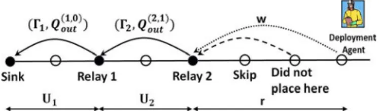
Fig. 2. Illustration of pure as-you-go deployment with and . In this “snap-shot” of the deployment process, the deployment agent has already placed Relay 1 and Relay 2 at distances and , has set their transmit powers to and , thereby achieving outage probabilities and (links shown by solid arrows). Having placed Relay 2, he skips the next location (since ); based on measurements made at the next location (dashed arrow), the algorithm advises him to not place a relay and move on. The diagram shows the agent in the process of evaluating the next location at distance from Relay 2 (dotted arrow). Based on these measurements, the deployment agent will decide whether to place a relay at ; if a relay is not placed here, it must be placed at the next location, since .
transmit power is a random variable, where the randomness comes from shadowing . Outage probability can be
mea-sured by sending a sufficiently large number of packets over a link and calculating the percentage of packets whose RSSI is
below .
B. Deployment Process and Related Notation
In this paper, we consider two approaches for deployment.
Pure as-you-go Deployment: After placing a relay, the agent
skips the next steps, and sequentially measures the outage probabilities from locations to the previously placed node, at all transmit power levels . As the agent explores the locations
and makes link quality measurements,2at each step he decides
whether to place a relay there, and if the decision is to place a relay, then he also decides the transmit power for the placed relay. This has been depicted in Fig. 2. In this process, if he has walked steps away from the previous relay, or if he encounters the source location, then he must place a node. and will be fixed before deployment begins.
Explore-Forward Deployment: After placing a node, the
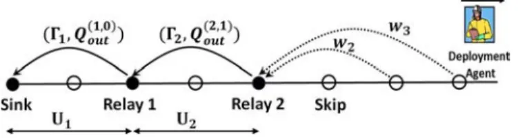
de-ployment agent skips the next locations and mea-sures the outage probabilities to the previous node from loca-tions , at each power level from the set . Then, based on these measurements3 of the outage
probability values, he places the relay at location
, sets its transmit power to , and repeats the same process for placing the next relay. This procedure is illustrated in Fig. 3. If the source location is encountered within steps from the previous node, then the source is placed.
Choice of and : If the propagation environment is very
good, or if we need to place a limited number of relays over a long line, it is very unlikely that a relay will be placed within the first few locations from the previous node. In such cases, we can skip measurements at locations and make mea-surements from locations . In general, the
2At a distance from the previous node, he measures the outage probabilities
from the current location to the previous node, where is the realization of the shadowing in the link being evaluated.
3Let us denote by the realization of shadowing in the potential link
between the -th location (starting from the previously placed node) and the previous node (see Fig. 3). The agent measures the outage probabilities in order to make a placement decision.
Fig. 3. Illustration of explore-forward deployment with and . In this “snap-shot” of the deployment process, the deployment agent has already placed Relay 1 and Relay 2 at distances and , has set their transmit powers to and , thereby achieving outage and (links shown by solid arrows). Having placed Relay 2, he skips the next location (since ). The agent then evaluates the next two locations (dotted arrows) . Then, based on the measurements at these two locations, the algorithm determines which of them to place the relay at and which power level to use.
choice of and will depend on the constraints and require-ments for the deployment. Larger will result in faster explo-ration, but very large will result in very high outage in each link. For a fixed , a large results in more measurements, but we can expect a better performance.
C. Traffic Model
In order to develop the problem formulation, we assume that the traffic is so low that there is only one packet in the network at a time; we call this the “lone packet model.” Hence, there are no simultaneous transmissions to cause interference. This per-mits us to easily write down the communication cost on a path over the deployed relays. However, this assumption does not trivialize the deployment problem, since the deployment must still take into account the stochastic shadowing and fading in the links, and the effects of these factors on the number of nodes de-ployed and the powers they use.
The lone packet traffic model is realistic for sensor networks that carry low duty cycle measurements, or just carry an occa-sional alarm packet. For example, recently there has been an effort to design passive infra-red (PIR) sensor platforms that can detect intrusion of a human or animal, and also can classify whether the intruder is a human or an animal ([15]). The data rate generated by such a platform deployed in a forest will be very low. The authors in [2, Section 3.2] use only a 1.1% duty cycle for a multi-hop wireless sensor network used for the pur-pose of wildlife monitoring. The sensors gather data from RFID collars on the animals; hence, the traffic to be supported by the network is light. Lone packet model is also realistic for condi-tion monitoring/industrial telemetry applicacondi-tions ([16]) as well, where the time between successive measurements is very large. Infrequent data model is common in machine-to-machine com-munication ([17]). Table 1 and Table 3 of [18] illustrate sensors whose sampling rate and the size of the sampled data packets are small; it shows data rate requirement as small as several bytes per second for habitat monitoring.
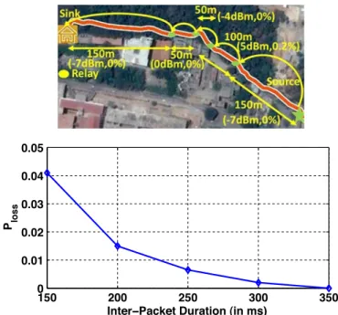
Even though the network is designed for the lone packet traffic, it will be able to carry some amount of positive traffic. See Section IX for experimental evidence of this claim; a five-hop line network deployed using one algorithm proposed in this paper, over a 500 m long line in a forest-like environ-ment, was able to carry 127 byte packets at a rate of 4 packets per second, with end-to-end packet loss probability less than 1%, which is sufficient for the applications mentioned above.
Lone packet model is also valid when interference-free com-munication is achieved via multi-channel access. Recently there have been efforts to use multiple channels available in 802.15.4
radio in a network; see [19]–[22]. In a line topology, this reduces to frequency reuse after certain hops, which, in turn, mitigates interference in the network. Thus, as with the lone packet as-sumption, the availability of multiple channels, and appropriate channel allocation over the network, eliminates the need to op-timize over link schedules.
It has been proved that design with the lone packet model can be the starting point for a design with desired positive traffic (see [23]). Network design for carrying a given positive traffic rate is left as a future research work.
D. Network Cost Structure
In this section we develop the cost that we use to evaluate the performance of a given deployment policy. Given the current location of the deployment agent with respect to the previous relay, and given the measurements made to the previous relay, a policy will provide the placement decision (in the case of pure as-you-go deployment, whether or not to place the relay, and if place then at what power, and in the case of explore-forward deployment, where among the locations to place the relay and at which power).
Let us denote the number of placed relays up to steps (i.e., meters) from the sink by ; define . Since deployment decisions are based on measurements to already placed relays, and since the path-loss over a link is a random variable (due to shadowing), we see that is a random process. In this paper we have assumed that each node for-wards each packet to the immediately previously placed relay (e.g., with reference to Fig. 1, the source forwards all packets to Relay 2, which, in turn, forwards all packets to Relay 1, etc.). See [11] for the considerably more complex possibility of relay skipping while forwarding packets.
When the node is placed, the deployment policy also pre-scribes the transmit power that this node should use, say, ; then the outage probability over the link , so created, is denoted by (see Fig. 2 and Fig. 3). We evaluate the cost of the deployed network, up to distance, as a linear combi-nation of three cost measures:
(i) The number of relays placed, i.e., .
(ii) The sum outage, i.e., . The motivation for this measure is that, for small values of , the sum-outage is approximately the probability that a packet sent from the point to the source encounters an outage along the path from the point back to the sink.
(iii) The sum power over the hops, i.e., .
These three costs are combined into one cost measure by combining them linearly and taking expectation (under a policy
), as follows:
(2) The multipliers and can be viewed as capturing the emphasis we wish to place on the corresponding measure of cost. For example, a large value of will aim for a network deployment with smaller end-to-end expected outage. We can view as the cost of placing a relay.
A Motivation for the Sum Power Objective: In case all the
nodes have wake-on radios, the nodes normally stay in sleep mode, and each sleeping node draws a very small current from the battery (see [24]). When a node has a packet, it sends a
wake-up tone to the intended receiver. The receiver wakes up and the sender transmits the packet. The receiver sends an ACK packet in reply. Clearly, the energy spent in transmission and reception of data packets governs the lifetime of a node, given that the ACK size is negligible. We assume that a fixed mod-ulation scheme is used, so that the transmission bit rate over all links is the same (e.g., in IEEE 802.15.4 radios, that are commonly used for sensor networking, the standard modulation scheme provides a bit rate of 250 Kbps). We also assume a fixed packet length. Let be the transmission duration of a packet over a link, and suppose that the node uses power during transmission. Let denote the packet recep-tion power expended in the electronics at any receiving node. If the packet generation rate at the source is very small, the life-time of the -th node is
seconds ( is the total energy in a fresh battery). Hence, the rate at which we have to replace the batteries in the network from the sink up to distance steps is given by
. The term can be absorbed into . Hence, the battery depletion rate is proportional to
.
E. Deployment Objective
We assume that the distance to the source from the sink is
a priori unknown, and its distribution is also unknown. Hence,
we assume that (deployment along a line of infinite length) and develop deployment policies that seek to minimize the average cost per step. This setting can be useful in practice
when is large (e.g., a long forest trail). Also, if we seek to create networks along multiple trails in a forest, and if deploy-ment is done serially along multiple trails, then this is effectively equivalent to deployment along a single long line, provided that the trails have statistically identical radio propagation environ-ment. Note that, in case we deploy serially along multiple lines but use this formulation, it means that we seek to optimize the per-step cost averaged over multiple lines.
1) Unconstrained Problem: Motivated by the cost structure
and the model, we seek to solve the following: (3) where is a placement policy, and is the set of all possible placement policies (to be formalized later). We formulate (3) as a long-term average cost Markov decision process (MDP).
2) Connection to a Constrained Problem: Note that, (3) is
the relaxed version of the following constrained problem where we seek to minimize the mean power per step subject to a con-straint on the mean outage per step and a concon-straint on the mean number of relays per step:
(4) The following standard result tells us how to choose the
La-grange multipliers and (see [25], Theorem 4.3):
Theorem 1: Consider the constrained problem (4). If there
exists a pair , and a policy such that is the optimal policy of the unconstrained problem (3) under
and the constraints in (4) are met with equality under , then is an optimal policy for (4) also.
III. PUREAS-YOU-GODEPLOYMENT
A. Markov Decision Process (MDP) Formulation
Here we seek to solve problem (3), for the pure as-you-go approach. When the agent is steps away from the previous node , he measures the outage prob-abilities on the link from the current location to the previous node, where is the realization of the shadowing random variable in the link being evaluated. He uses the knowledge of and the outage probabilities to decide whether to place a node at his current location, and what transmit power to use if he places a relay. In this case, we formulate the impromptu deployment problem as a Markov Decision Process (MDP) with state space
. At state
, the action is either to place a relay and select a transmit power, or not to place. When , the only feasible action is to place and select a transmit power . If, at state , a relay is placed and it is set to use transmit power , a hop-cost of
is incurred.4
A deterministic Markov policy is a sequence of mappings from the state space to the action space, and it is called a stationary policy if for all . Given the state (i.e., the measurements), the placement decision is made according to the policy.
B. Formulation for
Under the pure as-you-go approach, we will first minimize the expected total cost for , and then take
; this approach provides the policy structure for the average cost problem (see [26], Chapter 4).
In the case, the deployment process re-generates (probabilistically) after placing a relay, because of the memoryless property of the geometric distribution, and because of the fact that deployment of a new node will involve measure-ment of qualities of new links not measured before, and the new links have i.i.d. shadowing independent of the previously mea-sured links. The (special) state of the system at such regener-ation points is denoted by (apart from the states of the form ). When the source is placed at the end of the line, the process terminates. Suppose is the (random) number of re-lays placed, and node is the source node (as shown in Fig. 1). We first seek to solve the following:
(5) We will first investigate this approach assuming finite .
C. Bellman Equation
Let us denote the optimal expected cost-to-go at state and at state be and respectively. Note that here we have an infinite horizon total cost MDP with a finite state
4We have taken as a typical state for simplicity of
representa-tion; so long as the channel model given by (1) is valid, we can also take as a typical state. This happens because the cost of an action depends on the state only via the outage probabilities.
space and finite action space. The assumption P of Chapter 3 in [26] is satisfied, since the single-stage costs are nonnegative. Hence, by the theory developed in [26], we can focus on the class of stationary deterministic Markov policies.
By Proposition 3.1.1 of [26], the optimal value function satisfies the Bellman equation which is given by, for all
,
(6) These equations are understood as follows. If the current state is and the line has not ended yet, we can either place a relay and set its transmit power to
, or we may not place. If we place, the cost
is incurred at the current step, and the cost-to-go from there is . If we do not place a relay, the line will end with probability in the next step, in which case a
cost will be incurred.
If the line does not end in the next step, the next state will be a random state and a mean cost of will be incurred. At state the only possible decision is to place a relay. At state , the deployment agent starts walking until he encounters the source location or location ; if the line ends at step (with probability
), a cost of is
incurred. If the line does not end within steps (this event has probability ), the next state will be .
D. Value Iteration
The value iteration for (5) is obtained by replacing in (6) by on the L.H.S (left hand side) and by on the R.H.S (right hand side), and by taking for all states. The standard MDP theory says that for all states as .
E. Policy Structure: OptAsYouGo Algorithm
Lemma 1: is increasing in , and , de-creasing in , and jointly concave in and . is increasing and jointly concave in and .
Proof: See Appendix A.
Next, we propose an optimal algorithm OptAsYouGo (Op-timal algorithm with pure As-You-Go approach).
Algorithm 1: (OptAsYouGo Algorithm): At state
(where ), place a relay if and only
if , where
is a threshold increasing in . If
the decision is to place a relay, the optimal power to be se-lected is given by . At state , select transmit power
.
Theorem 2: Under the pure as-you-go approach, Algorithm 1 provides the optimal policy for Problem (3).
Proof: See Appendix A.
Remark: The trade-off in the impromptu deployment
problem is that if we place relays far apart, the cost due to outage increases, but the cost of placing the relays decreases. The intuition behind the threshold structure of the policy is that if at distance we get a good link with the combination of power and outage less than a threshold, then we should accept that link because moving forward is unlikely to yield a better link. is increasing in . Since is increasing in for any , and since shadowing is i.i.d across links, the probability of a link (to the previous node) having desired QoS decreases as we move away from the previous node. Hence, the optimal policy will try to place relays as soon as possible if is large, and this explains why is increasing in . Note that the threshold does not depend on , due to the fact that shadowing is i.i.d. across links.
F. Computation of the Optimal Policy
Let us write
, and . Also,
for each stage of the value iteration, define
and .
Multiplying both sides of the value iteration by and summing over , we obtain an iteration in terms of and this iteration does not involve . Since for each , and as , we can argue that
for all (by Monotone Convergence Theorem) and . Then we can compute by knowing itself (see the expression of in Algorithm 1); we need not keep track of the cost-to-go values for each state , at each stage . Here we simply need to keep track of . Similar iterations were proposed in [11] (Section III-A-5).
G. Average Cost Problem: Optimality of OptAsYouGo
Note that the problem (5) can be considered as an infinite horizon discounted cost problem with discount factor . Hence, keeping in mind that we have finite state and action spaces, we observe that for the discount factor sufficiently close to 1, i.e., for sufficiently close to 0, the optimal policy
for problem in (5) is optimal for the problem in (3) (see
[26, Proposition 4.1.7]). In particular, the optimal average cost per step with pure as-you-go approach, , is given by (see [26, Section 4.1.1]), where is the optimal cost for problem (5) under pure as-you-go with the probability of the line ending in the next step is .
In case is a Borel subset of , we still have a finite action space, and bounded, nonnegative cost per step. By [27, Theorem 5.5.4], one can show that the optimal average cost per step is again . As , we will obtain a sequence of optimal policies (i.e., mappings from the state space to the action space), and a limit point of them will be an average cost optimal policy.
H. HeuAsYouGo: A Suboptimal Pure As-You-Go Heuristic Algorithm 2: (HeuAsYouGo): The power used by the relays
is set to a fixed value. At each potential location, the deploy-ment agent checks whether the outage to the previous relay meets a certain predetermined target with this fixed transmit power level. After placing a relay, the next relay is placed at the last location where the target outage is met; or place at the -st location (after the previously placed relay) in the unlikely situation where the target outage is violated in the -st location itself. If the agent reaches the -th step and if all previous locations violate the outage target, he must place the next relay at step .
HeuAsYouGo is a modified version of the heuristic deploy-ment algorithm proposed in [5]. HeuAsYouGo is not exactly a pure as-you-go algorithm since it sometimes requires the agent to move one step back in case the outage target is violated.
IV. EXPLOREFORWARDDEPLOYMENT
A. Semi-Markov Decision Process (SMDP) Formulation
Let us recall explore-forward deployment from Section II-B; we denote by the realization of shadowing in the potential link between the -th location (starting from the previously placed node) and the previous node (see Fig. 3). The agent measures the outage probabilities
from locations
at all available transmit power levels from the set , in order to make a placement decision.
Here we seek to solve the unconstrained problem (3). We formulate our problem as a Semi-Markov De-cision Process (SMDP) with state space and action
space . The vector
, i.e., the shadowing from locations, is the state in our SMDP. In the state , an
action is taken
where is the distance of the next relay (from the previous relay) that would be placed and is the transmit power that this relay will use. In this case, a hop-cost of
is incurred. After placing a relay, the next state becomes with probability (since shadowing is i.i.d. across links).
Let us denote, by the vector , the (random) state at the -th decision instant, and by the action at the
-th decision instant. For a deterministic Markov policy , let us define the functions
and as follows: if
, then and .
B. Policy Structure: Algorithm OptExploreLim
Note that, is i.i.d across . The state space is a Borel space and the action space is finite. The hop cost and hop length (in number of steps) are uniformly bounded across all state-action pairs. Hence, we can work with stationary deter-ministic policies (see [28] for finite state space, i.e., finite , and [29] for a general Borel state space, i.e., when is a Borel set). Under our current scenario, the optimal average cost per step, , exists (in fact, the limit exists) and is same for all states . For simplicity, we work with finite , but the policy
structure holds for Borel state space also.
We next present a deployment algorithm called “OptExploreLim,” an optimal algorithm for limited exploration.
Algorithm 3: (OptExploreLim Algorithm:): In the state
which is captured by the measurements for , , place the new relay according to the stationary policy as follows:
(7) where (or ) is the optimal average cost per step for the Lagrange multipliers .
Theorem 3: The policy given by Algorithm 3 is optimal for the problem (3) under the explore-forward approach.
Proof: The optimality equation for the SMDP is given by
(see [28], Equation 7.2.2):
(8) is the optimal differential cost corresponding to state . The structure of the optimal policy is obvious from (8), since
does not depend on .
Later we will also use the notation or to denote the OptExploreLim policy under the pair ,
since here .
Remark 1: The same optimal policy structure will hold for a
Borel state space, by the theory presented in [29].
Remark 2: The optimal decision depends on state only via the outage probabilities which can be easily measured.
Remark 3: For an action , a cost
will be incurred. On the other hand, is the reference cost over steps. The policy minimizes the difference between these two for each link.
Remark 4: The policy requires the deployment agent to know
, and computation of will require perfect knowledge of propagation environment (e.g., the path-loss exponent in (1), the distribution of shadowing, etc.); see Section IV-C.
Theorem 4: is jointly concave, increasing and continuous in and .
Proof: See Appendix B.
Let us consider a sub-class of stationary deployment policies (parameterized by , and ) given by:
(9) where is not necessarily equal to .
Under the class of policies given by (9), let denote the sequence of inter-node distances, transmit powers and link outage probabilities that the optimal policy yields during the deployment process. By the assumption of i.i.d. shadowing across links, it follows that
is an i.i.d. sequence.
Let , and
denote the mean power per link, mean outage per link and mean placement distance (in steps) respectively, under the policy given by (9), where is not
necessarily equal to . Also, let , and denote the optimal mean power per link, the optimal mean outage per link and the optimal mean placement distance (in steps) respectively, under the OptExploreLim algorithm (i.e., policy
when in (9) is replaced by ). By the Re-newal-Reward theorem, the optimal mean power per step, the optimal mean outage per step, and the optimal mean number of relays per step are given by ,
and .
Theorem 5: For a given , the mean number of relays per step under the OptExploreLim algorithm (Algorithm 3), , decreases with . Similarly, for a given , the mean outage probability per step, , decreases with under the optimal policy.
Proof: See Appendix B.
Remark: The proof of Theorem 5 is quite general; the results
hold for the pure as-you-go approach also.
Theorem 6: For Problem (3), under the optimal policy (with
explore-forward approach) characterized by (i.e., under the OptExploreLim algorithm), we have
.
Proof: See Appendix B. C. Policy Computation
We adapt a policy iteration (from [28]) based algorithm to calculate . The algorithm generates a sequence of stationary policies (note that the notation was used for a dif-ferent purpose in Section IV-A; here each is a stationary, deterministic, Markov policy), such that for any ,
maps a state into some action. Define the sequence of functions as follows: if
, then and .
Algorithm 4: The policy iteration algorithm is as follows:
Step 1) (Initialization): Start with an initial policy . Step 2) (Policy Evaluation): Calculate the average cost
corresponding to the policy , for . is equal to the quantity (by the Renewal Reward The-orem) given by the expression at the bottom of the page.
Step 3) (Policy Improvement): Find a new policy by solving the following:
(10) If and are same (i.e., if ), then stop and declare , . Otherwise, go to Step 1.
Remark: By the theory in [28], this policy iteration will con-verge (to ) in a finite number of iterations, for finite state
and action spaces. For a general Borel state space (e.g., for
log-normal shadowing), only asymptotic convergence to can be guaranteed.
Computational Complexity: The finite state space has
cardi-nality . Then, addition operations are required to compute from the policy evaluation step. However, careful manipulation leads to a drastic reduction in this computational requirement, as shown by the following theorem.
Theorem 7: In the policy evaluation step in Algorithm 4, we
can reduce the number of computations in each iteration from
to .
Proof: See Appendix B.
D. HeuExploreLim: An Intuitive but Suboptimal Heuristic
A natural heuristic for (3) under the explore-forward ap-proach is the following HeuExploreLim Algorithm (Heuristic Algorithm for Limited Explore-Forward):
Algorithm 5: (HeuExploreLim Algorithm): Under the
ex-plore-forward setting as discussed in Section IV, at state , make the decision according to the following rule:
Under any stationary deterministic policy , let us denote the cost of a link by (a random variable) and the length of a link by (under any stationary deterministic policy , the deploy-ment process regenerates at the placedeploy-ment points).
Lemma 2: HeuExploreLim solves .
Proof: See Appendix B.
Remark: This heuristic is not optimal. Our optimal policy
given in Theorem (3) solves . How-ever, HeuExploreLim solves , which is, in general, different from . Note that
if and only if the variance of
is zero. But this does not happen due to the variability in shadowing over space.
V. COMPARISONBETWEENEXPLORE-FORWARD ANDPURE
AS-YOU-GOAPPROACHES
Let us denote the optimal average cost per step (for a given and ) under the explore-forward and pure as-you-go approaches by and .
Theorem 8: .
Proof: See Appendix C.
Next, we numerically compare various deployment algo-rithms, in order to select the best algorithm for deployment.
A. Parameter Values Used in the Numerical Comparisons
We consider deployment for a given and a given , for the objective in (3). We provide numerical results for de-ployment with iWiSe motes ([30]) (based on the Texas Instru-ment (TI) CC2520 which impleInstru-ments the IEEE 802.15.4 PHY in the 2.4 GHz ISM band, yielding a bit rate of 250 Kbps, with
a CSMA/CA medium access control (MAC)) equipped with 9 dBi antennas. The set of transmit power levels is taken to be dBm, which is a subset of the transmit power levels available in the chosen device. For the channel model as in (1), our measurements in a forest-like environment inside the Indian Institute of Science Campus gave path-loss exponent and (i.e., 1.7 dB); see [12]. Shadowing was found to be log-normal; with , where . Shadowing decorrelation distance was found to be 6 meters. Fading is assumed to be
Rayleigh; .
We define outage to be the event when the received signal power of a packet falls below (i.e., 97 dBm); for a commercial implementation of the PHY/MAC of IEEE 802.15.4, 97 dBm received power corresponds to a 2% packet loss probability for 127 byte packets for iWiSe motes, as per our measurements.
We consider deployment along a line with step size meters, , . Given , we chose is the following way. Define a link to be good if its outage probability is less than 3%, and choose to be the largest integer such that the probability of finding a good link of length is more than 20%, when the highest transmit power is used (this will ensure that the agent does not measure very long links having poor outage probabilities). For the parameters , , , and 5 dBm transmit power, turned out to be 5. If is increased further, the probability of getting a good link will be very small.
B. Numerical Comparison Among Deployment Policies
Assuming these parameter values, we computed (by MATLAB) the mean power per step (in mW), mean outage per step, mean placement distance (in steps), mean cost per step and mean number of measurements made per step, for the four deployment algorithms presented so far. The results are shown in Table I. In order to make a fair comparison, we
used the mean power per node for OptAsYouGo as the fixed node transmit power for HeuAsYouGo, and the mean outage per link of OptAsYouGo as the target outage for HeuAsYouGo.
The mean number of measurements per step is defined as the ratio of the mean number of links evaluated for deployment of one node and the mean placement distance (in steps). The numerator of this ratio is for explore-forward algorithms (since ). OptAsYouGo makes one measurement per step, but HeuAsYouGo makes more than one measurements per step since the agent often evaluates a bad link, takes one step back and places the relay.5
We notice that the average per-step cost (COST in Table I) of OptExploreLim (OEL) is the least. OEL uses the least mean power per step (POW column), places nodes the widest apart (DIST column), and the mean outage per step (OUT column) is second to lowest. On the other hand, OEL requires about twice as many measurements per step as compared to OptAsYouGo.6
Hence, we can conclude that the algorithms based on the ex-plore-forward approach significantly outperform the algorithms
5For planned deployment, we will have to evaluate all possible potential links;
from each potential location, we need to measure link quality to pre-ceding potential locations, which is not feasible.
6A more detailed comparison among the algorithms can be found in Appendix
C, along with elaborate discussion.
TABLE I
NUMERICALCOMPARISONAMONGVARIOUSALGORITHMS FOR AND . ABBREVIATIONS: OEL—OPTEXPLORELIM, HEL—HEUEXPLORELIM, OAYG—OPTASYOUGO, HAYG—HEUASYOUGO.
POW—MEANPOWER(INmW UNIT)PERSTEP, OUT—MEANOUTAGE PER
STEP, DIST—MEANPLACEMENTDISTANCE, COST—MEANCOST PERSTEP, MEAS—MEANNUMBER OFMEASUREMENTS PERSTEP
based on the pure-as-you-go approach, at the cost of slightly more measurements per step. Hence, for applications that do not require very rapid deployment, such as deployment along a long forest trail for wildlife monitoring, explore-forward is a better approach to take. Thus, for the learning algorithms presented later, we will consider only the explore-forward approach. How-ever, under the requirement of fast deployment (e.g., emergency deployment by first responders), pure as-you-go or deployment without measurements (as in [10]) might be more suitable.
VI. OPTEXPLORELIMLEARNING: LEARNINGWITH
EXPLORE-FORWARD,FORGIVEN AND
Based on the discussion in Section V, we proceed, in the rest of this paper, with developing learning algorithms based on the policy OptExploreLim (to solve problem (3)). We observe that the optimal policy (given by Algorithm 3) can be completely specified by the optimal average cost per step , for given values of and . But the computation of requires policy iteration. Policy iteration requires the channel model pa-rameters and , and it is computationally intensive. In prac-tice, these parameters of the channel model might not be avail-able. Under this situation, the agent measures
before deploying each relay, but he has to learn the optimal average cost per step in the process of deployment, and, use the corresponding updated policy each time he places a new relay. In order to address this requirement, we propose an algorithm which will maintain a running estimate of , and update it each time a relay is placed. The algorithm is motivated by the theory of Stochastic Approximation (see [31]), and it uses, as input, the measurements made for each place-ment, in order to improve the estimate of . We prove that, as the number of deployed relays goes to infinity, the running es-timate of average network cost per step converges to almost surely.
After the deployment is over, let us denote the length, transmit power and outage values of the link between node and node by , and . After placing the
-st node, we will place node , and consequently , and will be decided by the following algorithm.
Algorithm 6: (OptExploreLimLearning): Let be the es-timate of the optimal average cost per step after placing the -th relay (sink is node 0), and let be the initial estimate. In the process of placing relay , if the measured outage
prob-abilities are ,
After placing relay , update as follows (using the measurements made in the process of placing relay ):
(11) is a decreasing sequence such that ,
and . One example is .
Theorem 9: If we employ Algorithm 6 in the deployment
process, we will have almost surely.
Proof: By Theorem 6, under OptExploreLim, we have
; this leads to the stochastic approximation update in Algorithm 6. The detailed proof can be found in Appendix D.
While Algorithm 6 utilizes the general stochastic approxima-tion update, Algorithm 7 ensures that the iterate is the actual average network cost per step up to the -th relay.
Algorithm 7: Start with any . Let, for , be the average cost per step for the portion of the network already deployed between the sink and the -th relay, i.e.,
Place the -st relay according to the following policy:
Corollary 1: Under Algorithm 7 in the deployment process,
we will have almost surely.
Proof: See Appendix D.
VII. OPTEXPLORELIMADAPTIVELEARNING WITH
CONSTRAINTS ON OUTAGEPROBABILITY AND
RELAYPLACEMENTRATE
In Section VI, we provided a stochastic approximation al-gorithm for relay deployment, with given multipliers and , without knowledge of the propagation parameters. Let us recall that Theorem 1 tells us how to choose the Lagrange multipliers and (if they exist) in (3) in order to solve the problem given in (4). However, we need to know the radio propagation parameters (e.g., and ) in order to compute an optimal pair (if it exists) so that both constraints in (4) are met with equality. In real deployment scenarios, these propagation parameters might not be known. Hence, in this sec-tion, we provide a sequential placement and learning algorithm such that, as the relays are placed, the placement policy itera-tively converges to the set of optimal policies for the constrained problem displayed in (4). The policy is of the OptExploreLim type, and the cost of the deployed network converges to the op-timal cost. We modify the OptExploreLimLearning algorithm so that a running estimate gets updated each time a new relay is placed. The objective is to make sure that the running estimate eventually converges to the set of optimal tuples as the
deployment progresses. Our approach is via two time-scale sto-chastic approximation (see [31, Chapter 6]).
A. OptExploreLim: Effect of Multipliers and
Consider the constrained problem in (4) and its relaxed version in (3). We will seek a policy for the problem in (4) in the class of OptExploreLim policies (see (7)). Clearly, there exists at least one tuple for which there exists a pair such that, under the optimal policy , both constraints are met with equality. In order to see this, choose any and consider the corresponding optimal policy
(provided by OptExploreLim). Suppose that the mean outage per step and mean number of relays per step, under the policy , are and , respectively. Now, if we set the constraints and in (4), we obtain one instance of such a tuple .
On the other hand, there exist pairs which are not fea-sible. One example is the case (i.e., inter-node distance is always ), along with
, where is the maximum available transmit power level at each node. In this case, the outage con-straint cannot be satisfied while meeting the concon-straint on the mean number of relays per step, since even use of the highest transmit power at each node will not satisfy the per-step outage constraint.
Definition 1: Let us denote the optimal mean power per step
for problem (4) by , for a given . The set is defined as follows:
where the optimal average cost per step of the unconstrained problem (3) under OptExploreLim is .
can possibly be empty (in case is not a fea-sible pair). Hence, we make the following assumption which
en-sures the non-emptiness of .
Assumption 1: The constraint parameters and in (4) are such that there exists at least one pair for
which .
Remark: Assumption 1 implies that the constraints are
con-sistent (in terms of achievability). If , it would imply that both of the constraints are active. If , it would imply that we can keep the mean outage per step strictly less than by using the minimum available power at each node, while meeting the constraint on the relay placement rate. The optimal policy in Algorithm 3, under , will place re-lays with inter-relay distance steps, and use the min-imum available power level at each node. implies that the outage constraint cannot be met even with the highest power level at each node, under the relay placement rate con-straint. Similar arguments apply to .
We now establish some structural properties of .
Theorem 10: If is non-empty, then:
• Suppose that there exists , such that the policy satisfies both constraints in (4) with
equality. Then, there does not exist
satisfying (i) ,
and (ii) or
.
• If there exists a such that , then, ,
we have .
Proof: See Appendix E, Section A.
Assumption 2: The shadowing random variable has a con-tinuous probability density function (p.d.f.) over ; for any , . One example could be log-normal shadowing.
Theorem 11: Suppose that Assumption 2 holds. Under the
OptExploreLim algorithm, the optimal mean power per step , the optimal mean number of relays per step and the optimal mean outage per step , are continuous in
and .
Proof: See Appendix E, Section B.
Remark: Note that, by Theorem 11, we need not do any
ran-domization (see [32] for reference) among deterministic poli-cies in order to meet the constraints with equality.
B. OptExploreLimAdaptiveLearning Algorithm
Algorithm 8: This algorithm iteratively updates after each relay is placed. Let be the iterates after placing the -th relay (the sink is called node 0), and let be the initial estimates. In the process of deploying the -th relay, if the shadowing (which is measured indirectly only via
for and ) is
, then place the -th relay according to the following policy:
(12) After placing the -th relay, let us denote the transmit power, distance (in steps) and outage probability from relay to relay by , and . After placing the -th relay, make the following updates (using the measurements made in the process of placing the -th relay):
(13) where denotes the projection of on the interval . and need to be chosen carefully; the reason is explained in the discussion later in this section (along with a brief discussion on how and have to be chosen).
and are two decreasing sequences such that
, , , ,
and . In particular, we can
use and where , ,
.
Note that, for , we have . Let us define the set which is a subset of .
Theorem 12: Under Assumption 1, Assumption 2 and under
proper choice of and , the iterates in Algorithm 8 converge almost surely to as .
Proof: See Appendix E, Section C.
Remark: Algorithm 8 induces a nonstationary policy. But
Theorem 12 establishes that the sequence of policies generated by Algorithm 8 converges to the set of optimal stationary, de-terministic policies (for problem (4)).
Discussion of Theorem 12:
(i) Two timescales: The update scheme (13) can be rewritten as a two-timescale stochastic approximation (see [31], Chapter 6). Note that, , i.e., and
are adapted in a slower timescale compared to (which is adapted in the faster timescale). The dynamics behaves as if and are updated simultaneously in a slow outer loop, and, between two successive updates of and , we update in an inner loop for a long time. Thus, the update equation views and as quasi-static, while the and update equations view the update equation as almost equilibrated. (ii) Structure of the iteration: Note that,
is the excess outage compared to the allowed outage for the -th link. If this quantity is positive (resp., negative), the algorithm increases (resp., decreases) in order to reduce (resp., increase) the outage probability in subsequent steps. Similarly, if , the algorithm increases in order to reduce the relay placement rate. The goal is to ensure and
. In the faster timescale, our aim is to ensure that
.
(iii) Outline of the proof: The proof proceeds in five steps. We first prove the almost sure boundedness of . Next, we prove that the difference between the sequences and converges to 0 almost surely; this will prove the desired convergence in the faster timescale. This result has been proved using the theory in [31, Chapter 6] and Theorem 9.
In order to ensure boundedness of the slower timescale it-erates, we have used the projection operation in the slower timescale. We pose the slower timescale iteration in the same form as a projected stochastic approximation itera-tion (see [33, Equaitera-tion 5.3.1]).
In order to prove the desired convergence of the pro-jected stochastic approximation, we show that our iteration satisfies certain conditions given in [33] (see [33, Theorem 5.3.1]).
Next, we argue (using Theorem 5.3.1 of [33]) that the slower timescale iterates converge to the set of stationary points of a suitable ordinary differential equation (o.d.e.). But, in general, a stationary point on the boundary of the
closed set in the plane may not correspond to a point in . Hence, we will need
to ensure that if is a stationary point of the
o.d.e., then . In
order to ensure this, we need to choose and prop-erly. The choice of and is rather technical, and is explained in detail in Appendix E, Section C. Here we will just provide the method of choosing and ,
without any explanation of why they should be chosen in this way. The number has to be chosen so large that under and for all , we will have
for some small enough . We must also have . The number has to be chosen so large that for any , we will have (provided that ). The numbers and have to be chosen so large that there exists at least one
such that .
(iv) Asymptotic behaviour of the iterates: If the pair is such that one can be met with strict inequality and the other can be met with equality while using the optimal mean power per step for this pair , then one La-grange multiplier will converge to 0. This will happen if ; we will have (obvious from OptExploreLim with
) in this case. Here we will place all the relays at the -th step and use the smallest power level at each node. On the other hand, if the constraints are not feasible, then either or (since conver-gence to is not possible due to projection) or both will happen.
may have multiple tuples. But simulation results show that it has only one tuple in case it is nonempty.
C. Asymptotic Performance of Algorithm 8
Let us denote by the (nonstationary) deployment policy induced by Algorithm 8. We will now show that is an optimal policy for the constrained problem (4).
Theorem 13: Suppose that Assumption 1 and Assumption 2
hold. Then, under proper choice of and , the policy solves the problem (4); i.e., we have:
Proof: See Appendix E, Section D.
VIII. CONVERGENCESPEED OFLEARNINGALGORITHMS: A SIMULATIONSTUDY
In this section, we provide a simulation study to demon-strate the convergence rate of Algorithm 7 and Algorithm 8. The simulations are provided for , ,
, , , , ,
(see Section II for notation and Section V-A for parameter values).
Fig. 4. Demonstration of the convergence of OptExploreLimLearning (Algo-rithm 7) as deployment progresses. has not been included here.
A. OptExploreLimLearning for Given and
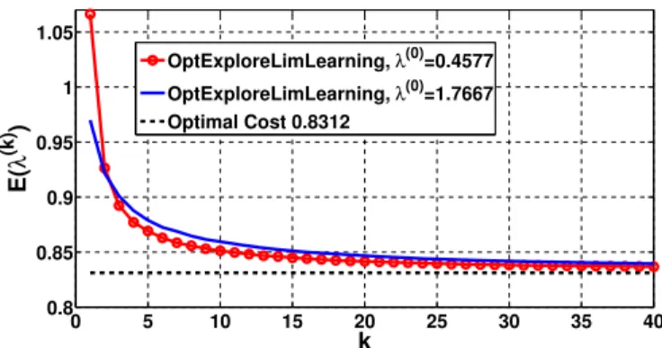
Let us choose , . We assume that the propagation environment in which we are deploying is char-acterized by the parameters as in Section V-A (e.g., , ). The optimal average cost per step, under these pa-rameter values, is 0.8312 (computed numerically).
On the other hand, for , , and , the optimal average cost per step is 0.4577, and it is 1.7667 for , . These two cases correspond to two different imperfect estimates of and available to the agent before deployment starts.
Suppose that the actual , , but at the time of deployment we have an initial estimate that , ; thus, we start with . After placing the -th relay, the actual average cost per step of the relay network connecting the -th relay to the sink is ; this quantity is a random vari-able whose realization depends on the shadowing realizations over the links measured in the process of deployment up to the -th relay. We ran 10000 simulations of Algorithm 7, starting with different seeds for the shadowing random process, and es-timating as the average of the samples of over these 10000 simulations. We also do the same for (op-timal cost for , ).
The estimates of as a function of , for the two initial values of , are shown in Fig. 4. Also shown, in Fig. 4, is the optimal value for the true propaga-tion parameters (i.e., , ). From Fig. 4, we observe that approaches the optimal cost 0.8312 for the actual propagation parameters, as the number of deployed re-lays increases, and gets to within 10% of the optimal cost by the time that 4 or 5 relays are placed, starting with two widely dif-ferent initial guesses of the propagation parameters. Thus, Op-tExploreLimLearning could be useful even when the distance can be covered by only 4 to 5 relays.
Note that, each simulation yields one sample path of the deployment process. We obtained the estimates of as a function of (by averaging over 10000 sample paths); the convergence speed will vary across sample paths even though
almost surely as .
B. OptExploreLimAdaptiveLearning
In this section, we will discuss how OptExploreLimAdap-tiveLearning (Algorithm 8) performs for deployment over a finite distance under an unknown propagation environment. We assume that the true propagation parameters are given in Section V-A (e.g., , ). If we know
the true propagation environment, then, under the choice and , the optimal average cost per step will be 0.8312, and this can be achieved by OptExploreLim (Algorithm 3). The corresponding mean outage per step will be (i.e., 0.1969%) and the mean number of relays per step will be 1/2.2859.
Now, suppose that we wish to solve the constrained problem in (4) with the targets (i.e., 0.1969%) and
, but we do not know the true propagation environ-ment. Hence, the deployment will use OptExploreLimAdap-tiveLearning with some choice of , and .
We seek to compare among the following three scenarios: (i) and are completely known (we use OptExploreLim with and in this case), (ii) imperfect estimates of and are available prior to deployment, and OptExplore-LimAdaptiveLearning is used to learn the optimal policy, and (iii) imperfect estimates of and are available prior to deploy-ment, but a corresponding suboptimal policy is used throughout the deployment without any update. For convenience in writing, we introduce the abbreviations OELAL and OEL for OptEx-ploreLimAdaptiveLearning and OptExploreLim, respectively. We also use the abbreviation FPWU for “Fixed Policy without Update.” Now, we formally introduce the following cases that we consider in our simulations:
(i) OEL: Here we know , , and use OptExploreLim (Algorithm 3) with ,
, . OEL will meet both the constraints with equality, and will minimize the mean power per step. (ii) OELAL Case 1: OELAL Case 1 is the case where the
true and (which are unknown to the deployment agent) are specified by Section V-A, but we use OptExploreLi-mAdaptiveLearning with , and , in order to meet the constraints specified earlier in this subsection. Note that, under and , the optimal mean cost per step is 0.5007 for , . Hence, we start with a wrong choice of Lagrange multipliers, a wrong estimate of and , and an estimate of the optimal average cost per step which cor-responds to these wrong choices. The goal is to see how fast the variables , and converge to the de-sired target 0.8312, 100 and 1, respectively. We also study how close to the desired target values are the quantities such as mean power per step, mean outage per step and mean placement distance for the relay network between
-th relay and the sink node.
(iii) OELAL Case 2: OELAL Case 2 is different from OELAL Case 1 only in the aspect that is used in OELAL Case 2. Note that, under and , the optimal mean cost per step is 1.7679
for , .
(iv) FPWU Case 1: In this case, the true and are unknown to the deployment agent. The deployment agent uses
, and throughout
the deployment process under the algorithm specified by (7). Clearly, he chooses a wrong set of Lagrange multipliers , , and he has a wrong estimate , . The optimal average cost per step is computed for these wrong choice of parameters, and the corresponding suboptimal policy is used throughout the deployment process without any
update; this will be used to demonstrate the gain in performance by updating the policy under OptExploreLi-mAdaptiveLearning, w.r.t. the case where the suboptimal policy is used without any online update.
(v) FPWU Case 2: It differs from FPWU Case 1 only in the aspect that we use in FPWU Case 2. Recall that, under and , the optimal mean cost per step is 1.7679 for , . For simulation of OELAL, we chose the step sizes as fol-lows. We chose , chose for the update and for the update (note that, both and are updated in the same timescale). We simulated 10000 independent network deployments (i.e., 10000 sample paths of the deployment process) with OptExploreLi-mAdaptiveLearning, and estimated (by averaging over 10000 deployments) the expectations of , , , mean power
per step , mean outage
per step and mean
placement distance , from the sink node to the -th placed node. In each simulated network deployment, we placed 20000 nodes, i.e., was allowed to go up to 20000. Asymptotically the estimates are supposed to converge to the values provided by OEL.
Observations From the Simulations: The results of the
simu-lations are summarized in Fig. 5. We observe that, the estimates of the expectations of , , , mean power per step up to the 20000th node, mean outage per step up to the 20000th node, and mean placement distance (in steps) over 20000 deployed nodes are 0.8551, 104.0606, 1.0385, 0.2005, 0.2% (i.e., 0.002) and 2.2939 for the OELAL Case 1, whereas those quantities are supposed to be equal to 0.8312, 100, 1, 0.1955, 0.1969% (i.e., 0.001969) and 2.2859, respectively. We found similar results for OELAL Case 2 also. Hence, the quan-tities converge very close to the desired values. We have shown
convergence only up to deployments in most cases, since the convergence rate of the algorithms in the initial phase are most important in practice.
All the quantities except expectation of and (which are updated in a slower timescale) converge reasonably close to the desired values by the time the 50th relay is placed, which will cover a distance of roughly 2–3.5 km. distance.
FPWU Case 1 and FPWU Case 2 either violate some con-straint or uses significantly higher per-step power compared to OEL. But, by using the OptExploreLimAdaptiveLearning al-gorithm, we can achieve per-step power expenditure close to the optimal while (possibly) violating the constraints by small amount; even in case the performance of OELAL is not very close to the optimal performance, it will be significantly better than the performance under FPWU cases (compare OELAL Case 2 and FPWU Case 2 in Fig. 5).
The speed of convergence will depend on the choice of the step sizes and ; optimizing the rate of convergence by choosing optimal step sizes is left for future endeavours in this direction. Also, note that, the choice of , and will have a significant effect on the performance of the network over a finite length; the more accurate are the estimates of and , and the better are the initial choice of , and , the better will be the convergence speed of OptExploreLimAdaptiveLearning.