Public Health Care Expenditures: Canada and the United States

(1)

Public Health Care Expenditures:

Canada and the United States

by David Boucher

david.boucher.1@umontreal.ca

Directed by François Vaillancourt

Département de Sciences Économiques Faculté des Arts et Sciences

(2)

ABSTRACT

This paper investigates the relationship between real per capita public health care expenditures and age distribution in Canada and the United States while controlling for other important factors. This study uses Province-level data for the period of 1981–2004 for Canada and state-level data for the time period of 1991-2004 are used for the USA. The main objective of the paper is to find a difference on Public Health Care expenditures between Canada and the US amongst the older age groups of the population (65 and over). Using DOLS (dynamic ordinarily least squares) and first-difference regressions for Canada and the US respectively, we find differences for several of the age groups. The most interesting result is that the age group of 65-69 yields a non-significant impact in Canada, but in the USA it yields a positive and significant effect on public health care expenditures. This is an important result because of the aging North-American population; it undoubtedly reflects the need for adequate health care policies in both countries, and particularly in the USA do to its effect on this particular age group.

(3)

As the world population ages, the impact of mass retirements and low fertility rates have raised concerns amongst many governments. Pensions, workforce and health care are the main issues targeted when analysing the issue future of aging in the developed countries. Because several countries support the elderly and the retirees (amongst others) through government programs, policy makers have to thoroughly analyse and anticipate the current and future costs of an aging population. In the current study, we try to depict the current Canadian and American situations regarding public health care and an increasingly older population. Using two separate

regressions, one DOLS (dynamic ordinarily least squares) regression for Canada and a first-difference regression for the United States, we analyze the effects of age and several control variables on public health care expenditures. We find that the distribution of age groups within a province/state has a significant effect on public health care expenditures. More interestingly, the population aged 65-69 has no impact in Canada, but has a positive impact in the USA on public health care expenditures. We believe that such an impact could be related to having universal health care access compared to only having government health care insurance coverage for the elderly and disabled (Medicare) and low income Americans (Medicaid). The essay is divided into three main sections: institutions and literature review, data & methodology and results.

(5)

1 – INSTITUTIONS AND LITERATURE REVIEW:

1.1 – INSTITUTIONS:

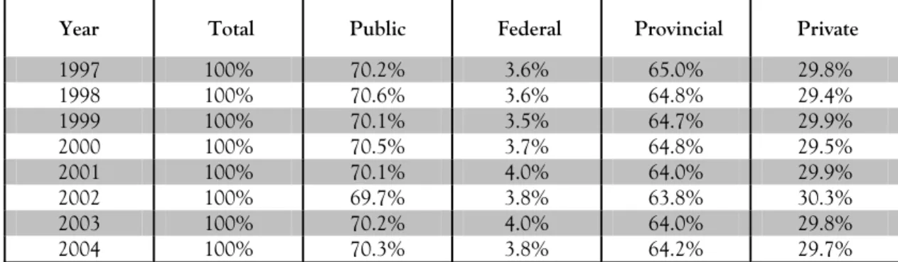
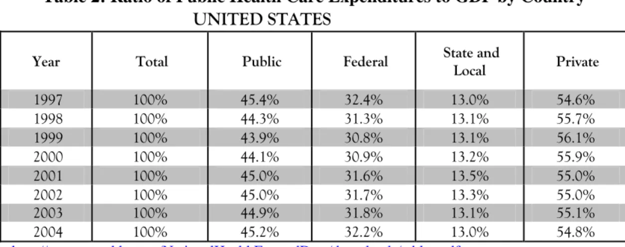
Since the current paper examines two countries in which health care systems differ greatly in both their type of services offered and health insurance coverage, we now briefly describe them focusing on the federal and provincial/state responsibilities. It should also be noted that there is an important distinction between Canada and the USA with regards to the shares of public health care expenditures. Table 1 presents how health insurance coverage differs from one country to the other: Canada, in 2004, has about 70.3% of its health care expenditures covered by a public source; whereas the USA have 45.2% covered by private sources. Also reflected in Table 1 and 2, in Canada, the federal government plays a much smaller role in terms of health care spending (3.8% in 2004) as it leaves most of the liability to the provinces (64.2% in 2004). In the United States, federal government assumes a larger share of the expenses (32.2% in 2004) and leaves the bulk to the private sector (54.8% in 2004), while the states handled the rest (13.0% in 2004).

Table 1: Ratio of Public Health Care Expenditures to GDP by Country CANADA

Year Total Public Federal Provincial Private

1997 100% 70.2% 3.6% 65.0% 29.8% 1998 100% 70.6% 3.6% 64.8% 29.4% 1999 100% 70.1% 3.5% 64.7% 29.9% 2000 100% 70.5% 3.7% 64.8% 29.5% 2001 100% 70.1% 4.0% 64.0% 29.9% 2002 100% 69.7% 3.8% 63.8% 30.3% 2003 100% 70.2% 4.0% 64.0% 29.8% 2004 100% 70.3% 3.8% 64.2% 29.7% Source: http://secure.cihi.ca/cihiweb/dispPage.jsp?cw_page=download_form_e&cw_sku=NHEXT7507PDF&cw_ctt=1&cw _dform=N

(6)

Table 2: Ratio of Public Health Care Expenditures to GDP by Country UNITED STATES

Year Total Public Federal State and _Local Private

1997 100% 45.4% 32.4% 13.0% 54.6% 1998 100% 44.3% 31.3% 13.1% 55.7% 1999 100% 43.9% 30.8% 13.1% 56.1% 2000 100% 44.1% 30.9% 13.2% 55.9% 2001 100% 45.0% 31.6% 13.5% 55.0% 2002 100% 45.0% 31.7% 13.3% 55.0% 2003 100% 44.9% 31.8% 13.1% 55.1% 2004 100% 45.2% 32.2% 13.0% 54.8% Source: http://www.cms.hhs.gov/NationalHealthExpendData/downloads/tables.pdf 1.1.1 – Canada

With some funding coming from the federal government, provinces administer their own health care programs. That is, they are responsible for the delivery of heath care services to their residents while being supported only in a financial manner by the Canadian government.

However the funding is conditional on certain criteria defined by the federal Canada Health Act (1984): comprehensiveness, universality, portability, accessibility and public administration.1 Briefly, those conditions are what define the universal access health care system in Canada. For instance it stipulates that health insurance must be comprehensive in covering all health care expenditures; it must be accessible to all Canadians without discrimination; as for portability, one resident of a specific province should be allowed the same coverage regardless of what province provides the health care services in Canada; and finally, health insurance is mandatory to be non-profitable and should be available to all residents of Canada regardless of their financial status. In order to finance their public health care systems, provinces use their own revenues and, as mentioned above, receive financial aid from the federal government. That is, “the Government of Canada provides significant financial support to provincial and territorial governments on an ongoing basis to assist them in the provision of programs and services. There are four main transfer programs: The Canada Health Transfer (CHT), the Canada Social Transfer (CST), Equalization and Territorial Formula Financing (TFF). The CHT and CST are federal transfers

1

(7)

which support specific policy areas such as health care, post-secondary education, social assistance and social services, early childhood development and childcare.”2

1.1.2 – United States

As opposed to Canada, where the provinces are the main entity providing health care services, the USA have both a federal and state public health care programs as well as private provision. The government health insurance is characterized by two components: Medicare and Medicaid (it also has a military component, but for the purpose of the analysis, it will be ignored).

MEDICARE: Medicare, the “Health Insurance for the Aged and Disabled”, is a federal

administered programme aimed at financially supporting the proportion of elderly and disabled populations. The programme is divided into four main parts (part A, B, C, and D) of coverage. Those parts define who is eligible for the public health insurance coverage and what type of services they are entitled to receiving:

• Part A helps pay for inpatient hospital, home health, skilled nursing facility, and

hospice care.

• Part B helps pay for physician, outpatient hospital, home health, and other services.

To be covered by Part B, all eligible people must pay a monthly premium.

• Part C, the Medicare Advantage program, expands beneficiaries’ options for

participation in private-sector health care plans.

• Part D provides subsidized access to prescription drug insurance coverage on a

voluntary basis, upon payment of premium, for all beneficiaries, with premium and cost-sharing subsidies for low-income enrolee3s.

It is to be noted that only part a “A” is free of premium charge, and «is generally provided automatically […] to persons age 65 or over who are eligible for Social Security or Railroad Retirement benefits, whether they have claimed these monthly cash benefits or not.4» As a result, Medicare is financed mostly by Medicare taxes, but also by the premiums paid by the enrolees who decide to expand their coverage.

2

Department of Finance Canada, http://www.fin.gc.ca/access/fedprove.html

3

Centers for Medicare and Medicaid Services, Brief Summaries of Medicare and Medicaid Title XVIII and Title XIX

of the Social Security Act, 2007

4

(8)

MEDICAID: Medicaid is a federal program with state-specific delivery which provides medical assistance to low income families in the USA. However, “[l]ow income is only one test for Medicaid eligibility for those within these groups; their financial resources also are tested against threshold levels (as determined by each State within Federal guidelines).5” Meaning that, not all low income residents are eligible for health care assistance. Also, “[s]tates generally have broad discretion in determining which groups their Medicaid programs will cover and the financial criteria for Medicaid eligibility.”6 This entitles states to manage their own expenditures based on political decisions.

Similarly to Canada, Medicaid is financed both at the state-level and at the federal level. FMAP (Federal Medical Assistance Percentage) can be viewed as the equivalent of federal health transfers in Canada. It is based on state-specific income and is determined annually by a formula that compares the State’s average per capita income level with the national income average7”. FMAP is therefore inversely related to per capita income.

An important note to consider is that states can also offer additional coverage to certain segments of the population through Medicaid. In fact, it can offer services to what the legal terms refers to as “categorically related” groups:

• Infants up to age 1 and pregnant women not covered under the mandatory rules whose family income is no more than 185 percent of the FPL. (The percentage amount is set by each State.)

• Children under age 21 who meet criteria more liberal than the AFDC income and resources requirements that were in effect in their State on July 16, 1996.

• Institutionalized individuals eligible under a “special income level.” (The amount is set by each State—up to 300 percent of the SSI Federal benefit rate.)

• Individuals who would be eligible if institutionalized, but who are receiving care under home and community-based services (HCBS) waivers.

• Certain aged, blind, or disabled adults who have incomes above those requiring mandatory coverage, but below the FPL.

• Aged, blind, or disabled recipients of State supplementary income payments. • Certain working-and-disabled persons with family income less than 250 percent of

the FPL who would qualify for SSI if they did not work.

• TB-infected persons who would be financially eligible for Medicaid at the SSI income level if they were within a Medicaid-covered category. (Coverage is limited to TB-related ambulatory services and TB drugs.)

• Certain uninsured or low-income women who are screened for breast or cervical cancer through a program administered by the Centers for Disease Control. The 5 Idem 6 Idem 7 Idem

(9)

Breast and Cervical Cancer Prevention and Treatment Act of 2000 (Public Law 106-354) provides these women with medical assistance and follow-up diagnostic services through Medicaid.

• “Optional targeted low-income children” included within the SCHIP program established by the BBA.

• “Medically needy” 8

In addition, Medicaid serves as a complement to Medicare for the elderly. Since the Balanced Budget Act (BBA) of 1997 Medicaid contains “a State option known as Programs of All-inclusive Care for the Elderly (PACE). PACE provides an alternative to institutional care for persons aged 55 or older who require a nursing facility level of care. The PACE team offers and manages all health, medical, and social services and mobilizes other services as needed to provide preventive, rehabilitative, curative, and supportive care. This care, provided in day health centers, homes, hospitals, and nursing homes, helps the person maintain independence, dignity, and quality of life.”

Finally, on top of the PACE, Medicaid can also be added to Medicare for the poor American residents:

Medicare beneficiaries who have low incomes and limited resources may also receive help from the Medicaid program. For such persons who are eligible for full Medicaid coverage, the Medicare health care coverage is supplemented by services that are available under their State’s Medicaid program, according to

eligibility category.9

As a whole, the Medicaid program offers flexibility to states in that they can use a proportion of the funding for certain populations if they are in need. For the purpose of this analysis, we note that Medicaid offers supplementary coverage for the elderly.

1.2 LITERATURE REVIEW:

1.2.1 – Populations and Health Expenditures:

As mentioned above, populations within Canada and the United States have been and will continue aging for years to come. That is, the proportions of elderly will continue to rise for both

8

Idem

9

(10)

Canada and the USA. Vaillancourt & Vochin (2007) have used data on the populations for Canada and the USA and shown through forecasts (1975-2030) that both of those populations will be characterized by an increasingly high proportion of residents aged 65 and over. This result has great implications for the interpretation of our analysis because our paper puts the emphasis on the effect of aging on public health care spending. Also, as seen in Figure I, Canada has been spending most of its financial resources dedicated to health care for its newborn and elderly populations. With regards to childbirth spending, the following figure does not tell the whole story, in that allocation for the newborns is distributed between the child and the mother in a specific manner. That is, when the child is born, the delivery, nursing, physician, and other costs will mostly be allocated to the mother10 while a small proportion of childbirth costs (related to direct care) will be allocated to the child. However a small portion of childbirth costs that is related to baby direct care (such as a nurse teaching the mother about feeding) will be allocated to the child. After which, all other costs (procedure for the newborn) will be attributed to the child.

Figure I: Total Provincial/Territorial Government Health Expenditure, Per Capita by Age, Canada, 2005

Source: CIHI, NHEX, http://secure.cihi.ca/cihiweb/dispPage.jsp?cw_page=statistics_results_source_nhex_e

10

(11)

Combining those two facts we should find corresponding effects of age on public health care expenditures in our regressions.

1.2.2 – Health Care Models:

As for health care expenditures models, there are a few recent studies that have looked at different factors and different methodologies when using panel data. Their key findings were considered while constructing the current analysis. Empirical literature on health care

expenditures has been mostly analysed from one point of view: income elasticity on total (public + private) expenditures. Ever since Newhouse (1977), researchers have tried to identify if health care was a luxury good, hence trying to examine income elasticity for health care expenditures. Much of the health expenditures determinants literature was dedicated to this issue. As a whole, those published conclude that there is a strong and positive relationship between GDP (Gross Domestic Product) and health care expenditures: Newhouse (1987), Parkin et al. (1987), Culyer (1990), Gerdtham and Jonsson (1991), Di Matteo (2000) and Di Matteo . Their methodologies basically consisted of a linear demand analysis using health care expenditures, GDP (or income) and a few control variables.

Much of the literature had ignored several important factors in determining health care

expenditures. Di Matteo (2005) tried to incorporate the effects of age and technology in order to remediate to this lack of potential factors that could play an important part in determining the latter. However, several of those studies have looked at time series and panel data, and proper methods are necessary to estimate, but they were often ignored. Other papers have tried to rigorously estimate health care expenditures using a battery of tests and adjusted methods. Hansen & King (1996) have tried to analyse the stationarity and cointegration of health care expenditures and GDP for 20 OECD countries using ADF (Augmented Dickey-Fuller) and EG (Engle-Granger) tests. They highlight the importance of testing for such bias as they find that several of the countries are facing non-stationarity in their expenditures and would therefore violate one of the hypotheses of the OLS. As a result, simple methods such as OLS would often be inadequate for the estimation of the relationship between health care and GDP. Based on that study, important pieces of literature followed: the works of Gerdtham & Lothgren (2000, 2002),

(12)

Dreger & Reimers (2005) and Morand Perrault & Vaillancourt (2007) brought rigorous evidence that further tests are needed to examine the relationship between health care expenditures, income and other important determinants.

Di Matteo (2005)

In his study, Di Matteo (2005) has tried to add explanatory variables to the estimation of the effects of income on health care expenditures in a comparative analysis between Canada and the United States. The author used two models in which he added age and technological variables. In the first model, the author attempts to model the share of the population of 65 and over and income on total health expenditures in separate regressions (one for each country). In the second, he incorporates more specific age groups (25-44, 45-64, 65-84 and 85+) as well as a time dummy to capture, in the author’s view, technological change in each country (the researcher also notes that the time dummy could account for other unwanted factors). The data ranges from 1980-1996 for the United States and 1975-2000 for Canada. In order to estimate the effects on the total health care expenditures within Canada and the United States, OLS (Ordinarily Least Squares) regressions are used for both countries. The author finds a significant impact ofthe proportion of elderly Canadians and Americans on health care spending. The findings suggest higher income elasticities for the United States than Canada in both models. When the time dummy is included in the second model, much of the effect of the population 65 and over is taken away.

Nonetheless, the author confirms that aging has a significant (but relatively modest) impact on health care expenditures, especially for the older age groups.

Gerdtham & Lothgren (2000, 2002)

Gerdtham & Lothgren (2000) have tested for Cointegration between GDP and health care expenditures using data on 21 OECD countries. The data ranges from 1960-1997. By taking a basic model of health expenditures and income, they expand the methodology in using unit root tests followed by a cointegration analysis. They commence the analysis by conducting ADF tests on each of the country’s health care expenses. While conducting the tests, they also reverse the null of cointegration and allow for a trend in the data. By comparing the series of tests for

(13)

cointegration, the authors find robust evidence of cointegration between health care expenditures and gross domestic product for the selected OECD countries and stress the importance of such procedures while using panel data. In a second attempt, Gerdtham & Lothgren (2002) supported their previous results by, once more, testing for cointegration between GDP and health care expenditures using data on 25 OECD countries. They began in the same manner, by conducting stationarity tests and followed with cointegration. Their new results show that the two variables are in fact cointegrated, but this time, they add that health spending and income are cointegrated around linear trends.

Dreger & Reimers (2005)

Further evidence of cointegration was provided by Dreger & Reimers (2005). The authors have contributed to the question by analyzing health care expenditures in 21 OECD countries while using different and more advanced econometric manipulations for panel data. The data ranges from 1975-2001. The LLC (Levin, Lin and Chu, 2002), and the IPS (Im, Pesaran and Shin, 2003) tests are used for stationarity tests. The LLC and IPS are generalizations of the ADF and are

applicable to panel data. As Dreger & Reimers estimate their version of the relationship between

health expenditures and income, they also include medical progress in their model. In order to find a good measure to approximate medical progress, they include life expectancy and infant mortality in different regressions for comparability. Moreover, the authors insert a methodology question in their analysis by comparing their results while using FMOLS (Pedroni, 1999) and DOLS (Mark and Sul, 2002), in order to find the most adequate procedure. Their results confirm cointegration relationships and positive impacts for income and medical progress. Their results also show that estimation methods for cointegration provide the same type of robust results.

Morand Perrault & Vaillancourt (2007)

Finally, Morand Perrault & Vaillancourt (2007) attempted to combine rigorous methods such as the ones used in Dreger & Reimers (2005) and expand their variable choice as Di Matteo (2005) had done. In addition, their model also included federal funding reforms in health care financing in both Canada and the United States. The data ranges from 1980-2004 in the United States and

(14)

1981-2003 in Canada. The study provides the same type of comparative analysis in Di Matteo (2005) as it analyses a battery of explanatory variables on total health care expenditures in separate regressions. As others have done, the authors followed the procedure to tests for stationarity in each of the variables, and if necessary, to test for cointegration between the non-stationary dependant variable and other non-non-stationary explanatory variables. After the tests concluded presence of non-stationarity and cointegration, they proceeded with DOLS regressions to take into account the existence of long-run relationships. Their results with regards to income concurred with those of previous studies in that it had strong positive impact in both countries. As for the age variable they found a positive impact of the population 65 and over in the United States, but could not conclude the same for Canada. Lastly, they found that the semi-elasticities for the reform dummy in the USA were smaller than those in Canada.

The results and methodologies of those studies were used to construct the current analysis. Borrowing different parts of each paper, our research narrows down the objective to analyzing the effects of aging for more age groups strictly on public health care expenditures by

province/state between two countries, Canada and the US. The following table presents an overview of the studies that were considered to build our model.

(15)

Table 3: Literature Review – Summary Author and

Year Subject Variables Methods Results

Di Matteo (2005)

Comparative analysis of the effects of income, age and time between Canada and the United States

Dependant variable: Real total personal health care expenditures per capita

Independent variables: income, age and time dummy

Multivariate regressions

• Found a significant impact ofthe proportion of elderly Canadians and Americans on health care spending. • Higher income elasticities for the United

States than Canada in both models. • Population 65 and over has less impact

when a time dummy is include, but still has a positive impact, especially for the older age groups.

Gerdtham & Lothgren (2000, 2002) Stationarity and cointegration between health expenditures and income in selected OECD countries Dependant variable: Total personal health care expenditures Independent variables: income,

Panel unit root tests, and panel cointegration tests

• Found robust evidence of cointegration between health care expenditures and gross domestic product for the selected OECD countries.

• New results show that the two variables are in fact cointegrated around linear trends. Dreger & Reimers (2005). Cointegration corrected regressions between health expenditures, income and medical progress in 21 OECD countries

Dependant variable: Total personal health care expenditures per capita Independent variables: income, life expectancy and infant mortality

Panel unit root tests, cointegration tests, dynamic ordinarily least squares and fully-modified ordinarily least squares

• Non-stationarity and confirm cointegration relationships.

• Positive impacts for income and medical progress. Morand Perreault & Vaillancourt (2007) Comparative cointegration corrected regressions between health care expenditures and income, age, transfers and reforms in Canada and the United States.

Dependant variable: Total personal health care expenditures per capita Independent variables: income, age, transfers, unemployment, reforms and health care price.

Panel unit root tests, cointegration tests and dynamic ordinarily least squares

• Confirm that income has a strong positive impact in both countries.

• Found a positive impact of the population 65 and over in the United States, but could not conclude the same for Canada. • Semi-elasticities for the reform dummy in

the USA were smaller than those in Canada.

(16)

2 – DATA AND METHODOLOGY

2.1 – THE MODEL:

The model used in the current analysis bases its choice of variables on a similar analysis in Di Matteo (2005). While using the same comparative type of methods, this paper tries to further investigate and understand the burden (if any) of aging on the public health care expenditures. Further, we also have investigated the presence of cointegration between public expenditures and a series of non-stationary variables. The methodology to complete such a task was borrowed from Dreger & Reimers (2005) and Morand Perreault & Vaillancourt (2007). However, we could not include a state/province-specific technological change variable robust enough due to the non availability of such a detailed level of analysis.

Using the methodologies from the papers previously mentioned, the general idea of our analysis can be summarized into two separate equations. The following explains each of the variables used and how they were implemented in estimating their effects on public health care by province/state:

PUBHCXn,t =

f

{ GDPn,t,PRIHCXn,t, HPRICEn,t, GINIn,t, TRANSFERSn,t, POP_RATIOSn,t }, n = 1,..., N; t = 1,…, T (1.1)

Public Expenditures (PUBHCX) are the real per capita public expenditures by province or by state depending on which country is analysed. For Canada, total public health care expenditures were used; for the US, Medicaid total expenditures were used as a proxy for health care

expenditures by state. This choice is based on the availability of the data and the fact that

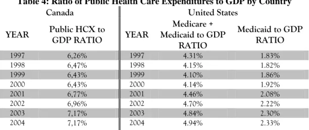
Medicaid consists of the highest proportion of public health care expenditures by state. Medicare expenditures are not included in the analysis because they are not state expenditures, they are a federal responsibility. The following table samples a few years to highlight the difference in the ratio of public health care expenditures to GDP in each country:

(17)

Table 4: Ratio of Public Health Care Expenditures to GDP by Country

Canada United States

YEAR Public HCX to _{GDP RATIO} YEAR

Medicare + Medicaid to GDP RATIO Medicaid to GDP RATIO 1997 6,26% 1997 4.31% 1.83% 1998 6,47% 1998 4.15% 1.82% 1999 6,43% 1999 4.10% 1.86% 2000 6,43% 2000 4.14% 1.92% 2001 6,77% 2001 4.46% 2.08% 2002 6,96% 2002 4.70% 2.22% 2003 7,17% 2003 4.84% 2.30% 2004 7,17% 2004 4.94% 2.33%

Source: CIHI, NHEX, http://secure.cihi.ca/cihiweb/dispPage.jsp?cw_page=statistics_results_source_nhex_e and http://www.cms.hhs.gov/NationalHealthExpendData/downloads/resident-state-estimates.zip

As shown in equation (1.1), a series of explanatory variables were used to estimate the effects on the public health care expenditures by province/state. The real per capita Gross Domestic Product (GDP), the real per capita private expenditures (PRIVHCX), the relative Health Care Price (HPRICE), the Gini Coefficient (GINI), Transfers for federal to province/state (TRANSFERS) and population ratios. It is to be noted that the private health care expenditures and transfers variables differ in Canada and United States (see section on DATA).

The model contains all variables in their logarithmic form. Based on the previous literature, logarithms are the most commonly used method to estimate health care spending at a

macroeconomic level. Further, Gerdtham and al. (1992) have found evidence supporting the logarithmic form for the estimated effects on health care spending using the Box-Cox tests for functional forms.

Regressions for panel data require several tests and adjustments according to their results. It is crucial to test for fixed or random effects, heteroskedasticity, correlation and autocorrelation within the data. More importantly, tests for stationarity and cointegration are required to adequately estimate the regressions. The section containing the results will show that public health care expenditures in Canada are non-stationary and that several of the Canadian

(18)

explanatory variables are non-stationary as well. Afterwards, cointegration tests will reveal a cointegrated relationship between the dependant variable and some of the non-stationary variables. The solution for the encountered results is to run DOLS (dynamic ordinarily least squares) in order to contain the effects of the cointegration relationship. Basically, the procedure consists of running the regression as described above while including the first-difference of the non-stationary explanatory variables as well as leads and lags of those first-differences. Usually, an information criterion can be used to calculate the appropriate number of lags to include, but due to the limited number of observations used, only one lead and one lag were included for the case of Canada. As for the USA, the results will show that the dependent variable is stationary around a trend, but several explanatory variables are non-stationary. Therefore, to control for the effect of the non-stationary variables, the regression will be estimated using all the variables (including the dependant) in their first-difference form.

2.2 – THE EXPECTATIONS:

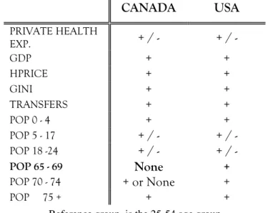
Based on the model, the following table presents the expected effect of each variable on public health care expenditures:

Table 5: Expected Effects on Public Health Care Expenditures by Province/State

_{CANADA USA} PRIVATE HEALTH EXP. + / - + / - GDP + + HPRICE + + GINI + + TRANSFERS + + POP 0 - 4 + + POP 5 - 17 + / - + / - POP 18 -24 + / - + / - POP 65 - 69 None + POP 70 - 74 + or None + POP 75 + + +

Reference group is the 25-54 age group

Private Health care expenditures could have a positive or negative impact on public health care expenditures depending on the relationship between the two; it could either be a substitute, which

(19)

would result in a negative coefficient; or it could be a complement, which would result in a positive coefficient (meaning that private expenditure would generate public expenditure).

As for GDP, we have already presented a number of studies that have found a positive and significant effect on total health care expenditures; therefore, we expect public health care expenditures to be similarly affected by GDP.

Relative health care price would also yield a positive effect due to the link between health care costs and health care expenditures. That is, significantly higher health care price would require significantly higher revenue to compensate for the augmentation.

For the Gini coefficient, the hypothesis is that higher income inequality within a province or a state would create a larger demand for public spending to help the poor. Therefore, the

relationship should be positive.

Federal transfers are expected to yield a similar effect as the Gini coefficient, meaning that

province/states who received larger transfers (or FMAP for the USA) are expected to spend more on health either as a result of the formula or as a result of the implicit reduction in costs of doing so.

Now, for the population ratios. As shown in Figure 1, certain age groups require more medical attention than others. Among those, the newborns and the elderly are two of the groups that should drive up health care costs. Therefore, we expect the population ratios’ coefficients to reflect such an effect. As for our comparative study, we should find similar results for Canada and the USA. However, our hypothesis is that due to the difference in health care systems, certain age groups will generate higher/lower public costs. More accurately, in the USA results, we should obtain non-significant coefficients for the age groups of 55-59 and 60-64 followed by a strongly positive coefficient for the age group of 65-69 (refer to Section on institutions for more details on Medicaid expenditures for the elderly); as opposed to finding non-significant

coefficients for all the above mentioned age groups for the Canadian results. That is, this paper assumes that in the USA, instead of paying for health care (through private firms), age groups of

(20)

55-59 and 60-64 will postpone whatever health care needs they have until they qualify for government insurance coverage and take advantage of the state funded program to finally take care of their medical needs.

2.3 – THE DATA:

The data for Canada ranges from 1981-2004 including all ten provinces (i.e., excluding the territories). As for the USA, the data ranges from 1991-2004 for the 50 states. Several data sources were used in order to construct the appropriate database. Table 6 summarises the variables used and the sources.

Table 6: Data Description and Sources Used for Canada and the US

_{Canada United}

_States

Health Care Expenditures

The public health care expenditures were obtained from CIHI (Canadian Institute for Health Information). Data contains total public health care expenditures for all ten provinces. Using province-specific CPI (Consumer Price Index) and population data, the variable was transformed to a real per capita form.

The public health care expenditures were obtained from CMS (Centres for Medicare & Medicaid

Services). The variable contains total Medicaid expenditures by state of residence. Using region-specific CPI and state population data, the variable was transformed to a real per capita form.

Private Expenditures

The private health care expenditures were obtained from CIHI. Data contains total private health care expenditures for all ten provinces. Using province-specific CPI and population data, the variable was transformed to a real per capita form.

The private health care

expenditures were obtained from CMS. The variable was constructed by taking total aggregate

expenditures by state of residence and subtracting Medicare & Medicaid by state of residence. Using region-specific CPI and state population data, the variable was transformed to a real per capita form.

(21)

Canada United

States

GDP

The nominal gross domestic product was obtained from Statistics

Canada’s CANSIM (Canadian Socio-economic Information Management System) provincial accounts table. Using province-specific CPI and population data, the variable was transformed to a real per capita form.

The nominal gross domestic product was obtained from the BEA (Bureau of Economic Analysis). Using region-specific CPI and state population data, the variable was transformed to a real per capita form.

HPRICE

The relative health care price was obtained from CANSIM. It was then deflated by the province-specific CPI to obtain the relative health care price.

N/A

GINI

The Gini coefficient was obtained from CANSIM. It represents a measure of income inequality within a specific province.

The Gini coefficient was obtained from census bureau. It represents a measure of income inequity within a specific state.

TRANSFERS

The federal transfers were obtained from CANSIM. It represents the total amount the federal government allocates each province. Using province-specific CPI and population data, the variable was transformed to a real per capita form.

The FMAP (The Federal Medical Assistance Percentages) was obtained from the United States Department of Health & Human Services. It represents the

percentage of Medicaid paid out of federal funds for Medicaid (see health care systems for broader description).

CPI

The consumer price index was obtained from CANSIM for every province (1997=100)

The consumer price index was obtained from the census bureau. However, there is no measure for a state specific CPI, therefore a regional CPI was used instead

POPULATION

Population data was obtained from CANSIM for all ten provinces. Age groups ratios were then create for the following age groups:

0 – 4, 5 – 17, 18 – 24, 25 – 54, 55 – 59, 60 – 64, 65 – 69, 70 – 74, 75 +.

Population data was obtained from the Census Bureau for all states. Age groups ratios were then create for the following age groups:

0 – 4, 5 – 17, 18 – 24, 25 – 54, 55 – 59, 60 – 64, 65 – 69, 70 – 74, 75 +.

(22)

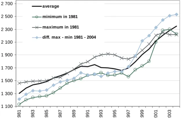
Figure IV - VII provide a few details on the behaviour of both the public health care expenditure throughout the years of 1981-2004 for Canada and 1991-2004 for the United States. All

provinces and states share the overall positive trend in their expenditures. However, unit root tests will be necessary to further investigate this tendency. To better understand how real per capita public health care expenditures are distributed throughout the provinces and the states, we refer to Appendix A and Appendix B for an overview of the variation of public health care spending in both countries.

The following figures provide an overview of the dependant variables and the ratio of residents aged 65+ over the entire population in Canada and the United States:

Figure IV: Distribution of Real per capita Public Health Care Expenditures in Canada, 1981-2004 1 100 1 300 1 500 1 700 1 900 2 100 2 300 2 500 2 700 1981 1983 1985 1987 1989 1991 1993 1995 1997 1999 2001 2003 average minimum in 1981 maximum in 1981

diff. max - min 1981 - 2004

Note: Average represents the average of real per capita public health care expenditures for the 10 provinces; minimum in 1981 = P.E.I.; maximum in 1981 = B.C.; diff. max – min represents the difference between the largest amount of expenditures and the lowest amount of expenditures for the corresponding year.

(23)

Figure V: Distribution of Real per capita Public Health Care Expenditures in the United States, 1981-2004 0 200 400 600 800 1 000 1 200 1991 1992 1993 1994 1995 1996 1997 1998 1999 2000 2001 2002 2003 2004 average minimum in 1991 maximum in 1991

diff. max - min 1991 - 2004

Note: Average represents the average of real per capita public health care expenditures for the 50 states; minimum in 1991 = Nevada; maximum in 1991 = New York; diff. max – min represents the difference between the largest amount of expenditures and the lowest amount of expenditures for the corresponding year.

For both Canada and the USA, we notice an upward trend in public health care expenditures. In Canada, P.E.I. had the lowest real per capita health care expenditures in 1981, but in 2004, it became the province of Quebec. British-Columbia had the highest level of expenditures in 1981, but Manitoba topped the chart in 2004. As for the United States, lowest amount in 1991 and 2004 was for Nevada. The highest amount for 1991 and 2004 was found in the state of New York. As it appears in the previous two graphs, the difference between the maximum amount spent and the lowest amount spent in a province or state seems to increase over time.

(24)

Figure VI: Share of residents aged 65+ over the total population in Canada, 1981-2004 6% 7% 8% 9% 10% 11% 12% 13% 14% 1981 1982 1983 1984 1985 1986 1987 1988 1989 1990 1991 1992 1993 1994 1995 1996 1997 1998 1999 2000 2001 2002 2003 2004 average max in 1981 max in 2004 min in 1981 and 2004 Note: Average represents the average of the ratio of the population aged 65+ over the entire population in the

corresponding province; minimum in 1981 = minimum in 2004 = Alberta; maximum in 1981 = P.E.I.; maximum in 2004 = Saskatchewan.

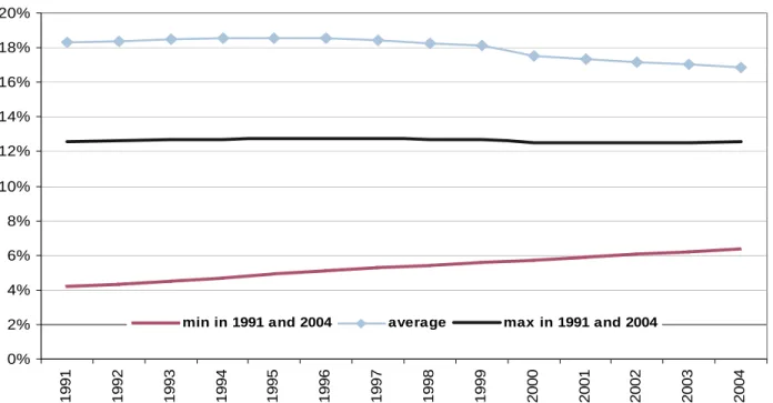
Figure VII: Distribution of the ratio of residents aged 65+ over the total population in the United States, 1981-2004 0% 2% 4% 6% 8% 10% 12% 14% 16% 18% 20% 19 91 19 92 19 93 19 94 19 95 19 96 19 97 19 98 19 99 20 00 20 01 20 02 20 03 20 04

min in 1991 and 2004 average max in 1991 and 2004

Note: Average represents the average of the ratio of the population aged 65+ over the entire population in the

corresponding province; minimum in 1991 = minimum in 2004 = Alaska; maximum in 1991 = maximum in 2004 = Florida.

(25)

In the previous figures, we notice that Canada’s upward trend is more evident that the USA, but as mentioned in the literature review, populations aged 65 and over should continue to rise significantly in Canada and the USA (refer to Vaillancourt & Vochin (2007) for more details on this issue). The province with the lowest ratio of residents aged 65 and over in both 1981 and 2004 is Alberta. As for the highest ratio, P.E.I. contained the highest in 1981 and Saskatchewan topped the chart in 2004. South of the border, Alaska contained the lowest ratio in both 1991 and 2004 and Florida detained the highest also for 1991 and 2004.

Other variables that were not found in the previous studies have been incorporated in our analysis: the Gini coefficient and real per capita federal transfers or FMAP (depending on the country). This short section will provide a few details on those variables. In 1981, the province of Newfoundland had the lowest Gini coefficient (0.327) of the Canadian provinces and

Saskatchewan was the province with the highest coefficient (0.376). In 2004, PEI became the province with the lowest Gini coefficient (0.342) while British-Columbia topped the chart (0.400). As a whole, the average for the ten provinces increased from 0.348 to 0.376 for the time period of 1981 to 2004. As for the United States, Connecticut had the lowest Gini coefficient in 1991 (0.365) while Louisiana had the highest (0.456). In 2004, the state of Alaska had the lowest coefficient (0.400) and New York became the state with highest (0.511). Overall, the United States average augmented from 0.412 to 0.449 for the period of 1991 to 2004.

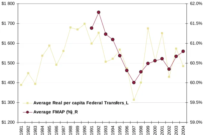
Finally, we provide a few details on the real per capita federal transfers and the FMAP. In Canada, Saskatchewan was the province that received the lowest amount of federal transfers in 1981, but, in 2004, it was Ontario. PEI was the province that received the largest amount of federal transfers in 1981 and 2004. The following chart highlights the fact that the average real per capita federal transfers have fluctuated over time, but the difference from 1981 to 2004 is quite small.

(26)

Figure VIII: Average of the real per capita Federal Transfers in Canada, 1981-2004 and FMAP in the United States, 1991-2004

$1 200 $1 300 $1 400 $1 500 $1 600 $1 700 $1 800 19 81 19 82 19 83 19 84 19 85 19 86 19 87 19 88 19 89 19 90 19 91 19 92 19 93 19 94 19 95 19 96 19 97 19 98 19 99 20 00 20 01 20 02 20 03 20 04 59.0% 59.5% 60.0% 60.5% 61.0% 61.5% 62.0%

Average Real per capita Federal Transfers_L Average FMAP (%)_R

Note: Average represents the average of the real per capita transfer payments/FMAP for all 10 provinces/50 states.

For the FMAP, a few of the states had the minimum ratio of 50% in 1991: Alaska, California, Connecticut, Delaware, Illinois, Maryland, Massachusetts, Nevada, New Hampshire, New Jersey, New York, Virginia. In 2004, we find a lot of the same states at the 50% (minimum) threshold level: California, Colorado, Connecticut, Delaware, Illinois, Maryland, Massachusetts,

Minnesota, New Hampshire, New Jersey, New York, Virginia and Washington. Again in 2004, Mississippi topped the chart with a ratio of 77.08%, however, at a lower ratio than in 1991. Overall, the FMAP varies over our time span.

(27)

3 – RESULTS

3.1 – HETEROSKEDASTICITY AND CORRELATION:

A battery of tests is introduced in this section in order to undertake valid and robust regressions. As previously mentioned, heteroskedasticity, contemporaneous correlation and serial correlation problems must be examined when using panel data. First, a Breush-Pagan test is used to detect heteroskedasticity in the residuals. Secondly, to test for the presence of contemporaneous correlation, we use another Breush-Pagan procedure. Finally, the issue of serial correlation is identified using a Wooldridge test. Table 7 summarizes the tests along with their outcome under the null and the alternative. As a whole, all the tests aside from one (fixed effects for the USA) were rejected. As noted in the following table, corrections are needed in order to proceed with unbiased regressions.

Table 7: Heteroskedasticity and Correlation Tests Results

Test

H0 Outcome Interpretation Outcome Interpretation

Fixed vs. random effects

Independence between residuals and explanatory variables

Rejects H0 Fixed effects are to be used in the analysis

Does not reject H0

Random effects are to be used in the analysis

Heteroskedasticity Homoskedasticity Rejects H0 Possible presence of Heteroskedasticity. Second test needed.

Rejects H0 Possible presence of Heteroskedasticity. Second test needed.

Heteroskedasticity (individuals)

Homoskedasticity Rejects H0 Presence of Heteroskedasticity between individuals. Correction needed Rejects H0 Presence of Heteroskedasticity between individuals. Correction needed Correlation no cross-sectional correlation Rejects H0 Contemporaneous correlation Rejects H0 Contemporaneous correlation

Serial correlation no first-order correlation Rejects H0 Presence of serial correlation. Correction needed

Rejects H0 Presence of serial correlation. Correction needed

(28)

3.2 – UNIT ROOTS:

Based on several of the articles mentioned in the literature review, unit root and cointegration tests were deemed essential. By following what Dreger & Reimers (2005) have done, we consider the LLC (Levin, Lin and Chu, 2002), the IPS (Im, Pesaran and Shin, 2003) tests. The LLC and IPS and based on ADF stats, as mentioned above, they are generalizations of the latter and are applied to panel data. The null hypothesis for all the unit root tests used in the current analysis is the presence of

a unit root. As Dreger & Reimers (2005) mention, the proper way to estimate the optimal lag

length is using an information criterion. However, due to our small sample, we only included one lag to preserve the power of the tests. Table 8 & 9 contain all the results of the unit root tests at a 95% confidence interval.

3.2.1 Canadian Tests:

Table 8: Unit Root Tests Results for Canada

Variable Statistics Unit Root _Tests Variable Statistics Unit Root _Tests

Levin-Lin t-rho-_stat Does not Reject POP5_17 Levin-_Lin t-rho-_stat Does not Reject Levin-Lin

ADF-stat Does not Reject

Levin-Lin

ADF-stat Does not Reject PUBLIC

EXPENDITURES

IPS ADF-_stat Does not Reject IPS ADF-_stat Does not Reject Levin-Lin t-rho-_stat Does not Reject POP18_24 Levin-_Lin t-rho-_stat Does not Reject Levin-Lin ADF-_stat Does not Reject Levin-_Lin ADF-_stat Reject PRIVATE

EXPENDITURES

IPS ADF-_stat Reject IPS ADF-_stat Reject Levin-Lin t-rho-_stat Does not Reject POP55_59 Levin-_Lin t-rho-_stat Does not Reject Levin-Lin

ADF-stat Does not Reject

Levin-Lin

ADF-stat Does not Reject GDP

IPS ADF-_stat Does not Reject IPS ADF-_stat Reject Levin-Lin t-rho-_stat Does not Reject POP60_64 Levin-_Lin t-rho-_stat Reject Levin-Lin ADF-_stat Does not Reject Levin-_Lin ADF-_stat Does not Reject TRANSFERS

IPS ADF-_stat Does not Reject IPS ADF-_stat Does not Reject Levin-Lin

t-rho-stat Does not Reject POP65_69

Levin-Lin

t-rho-stat Reject Levin-Lin ADF-_stat Does not Reject Levin-_Lin ADF-_stat Does not Reject HEALTH CARE

PRICE

(29)

Table 8 continued

Levin-Lin t-rho-_stat Reject POP70_74 Levin-_Lin t-rho-_stat Does not Reject Levin-Lin ADF-_stat Reject Levin-_Lin ADF-_stat Does not Reject GINI

IPS

ADF-stat Reject IPS

ADF-stat Does not Reject Levin-Lin t-rho-_stat Does not Reject POP75 Levin-_Lin t-rho-_stat Does not Reject Levin-Lin ADF-_stat Does not Reject Levin-_Lin ADF-_stat Does not Reject POP0_4

IPS ADF-_stat Does not Reject IPS ADF-_stat Does not Reject H0: Unit root; all results are reported at a level of 5%

The previous table shows results from the LLC and IPS Tests for unit root for the Canadian data. As we are unable to reject for most of the variables, including the dependant variable, we must pursue our investigation with cointegration tests. We already know from the previous studies cited in the introduction, that there is a strong possibility of cointegration between GDP and health care expenditures. However, because we are using a series of other I(1) variables, they must also be included in our cointegration tests. The next subsection will outlay an analysis of the subject.

(30)

3.2.1 United States Tests:

Table 9: Unit Root Tests Results for United States

Variable Statistics Unit Root _Tests Variable Statistics Unit Root _Tests

Levin-Lin t-rho-stat Rejects Levin-_Lin t-rho-stat Does Not Reject Levin-Lin ADF-stat Rejects Levin-_Lin ADF-stat Does Not Reject PUBLIC

EXPENDITURES

IPS ADF-stat Rejects

POP5_17

IPS ADF-stat Does Not Reject Levin-Lin t-rho-stat Rejects Levin-_Lin t-rho-stat Does Not Reject Levin-Lin ADF-stat Rejects Levin-_Lin ADF-stat Does Not Reject PRIVATE

EXPENDITURES

POP18_24

IPS ADF-stat Rejects Levin-Lin t-rho-stat Does Not Reject Levin-_Lin t-rho-stat Does Not Reject Levin-Lin ADF-stat Does Not Reject

Levin-Lin ADF-stat Does Not Reject GDP

IPS ADF-stat Does Not Reject

POP55_59

IPS ADF-stat Rejects Levin-Lin t-rho-stat Does Not Reject Levin-_Lin t-rho-stat Rejects Levin-Lin ADF-stat Does Not Reject Levin-_Lin ADF-stat Rejects FMAP

POP60_64

IPS ADF-stat Rejects Levin-Lin t-rho-stat Rejects Levin-_Lin t-rho-stat Does Not Reject Levin-Lin ADF-stat Rejects Levin-_Lin ADF-stat Does Not Reject GINI

POP65_69

IPS ADF-stat Does Not Reject Levin-Lin t-rho-stat Does Not Reject Levin-_Lin t-rho-stat Does Not Reject Levin-Lin ADF-stat Does Not Reject Levin-_Lin ADF-stat Does Not Reject POP0_4

POP70_74

Levin-Lin t-rho-stat Does Not Reject

Levin-Lin ADF-stat Does Not Reject POP75

IPS ADF-stat Rejects H0: Unit root; all results are reported at a level of 5%

The previous table shows results from the LLC and IPS Tests for unit root for the US data. We notice that the dependant variable appears to be stationary (around a trend). As for most of the explanatory variables, we cannot reject the null unit root. Contrary to Canada, our regression for the US will not be estimated between a I(1) dependant variable and a series of I(1) explanatory, therefore, there is no need to further investigate for cointegration. However, the US regression will have to be adjusted in a manner that it will be controlled for the non-stationarity effect of the explanatory variables. The solution that we have considered is to estimate the regression in the

(31)

first difference form for all the variables (including the dependant). The regressions results section contains further details on the subject.

3.3 – COINTEGRATION:

Cointegration tests for panel data was taken from the tests suggested in Pedroni (1999). They consist of adjusted EG (Engle-Granger) test (1987) for panel data. They are based on ADF and PP (Phillips-Perron) tests. The null hypothesis for all cointegration tests used in the current analysis is the absence of cointegration. Table 10 & 11 present the results for cointegration in Canadian data. Due to a high number of non-stationary variables, several tests were used to capture the presence of cointegration. However, due to an anomaly in the regression results for Canada (see section below), two datasets were used for cointegration tests: the first includes all variables presented earlier in the text; the second excludes federal transfers.

Table 10: Cointegration Tests Results for Canada

Variable Statistics Cointegration Tests

panel v-stat Does not Reject

panel rho-stat Rejects

panel pp-stat Rejects

panel adf-stat Rejects

group rho-stat Rejects

group pp-stat Does not Reject HCXPUB,

HCXPRIVATE, GDP, TRANSFERS, HPRICE,

POP75R

group adf-stat Rejects

panel v-stat Does not Reject panel rho-stat Does not Reject

panel pp-stat Rejects

panel adf-stat Rejects

group rho-stat Rejects

group pp-stat Rejects

HCXPUB, HCXPRIVATE, GDP,

FEDTRANSFERS, POP75

group adf-stat Rejects

(32)

Table 11: Alternative Cointegration Tests Results for Canada – Excluding Transfers

Variable Statistics Cointegration Tests

panel v-stat Does not Reject panel rho-stat Does not Reject panel pp-stat Does not Reject

panel adf-stat Reject

group rho-stat Does not Reject group pp-stat Does not Reject HCXPUB, GDP,

HPRICE, POP75

group adf-stat Reject

panel v-stat Does not Reject panel rho-stat Does not Reject panel pp-stat Does not Reject

panel adf-stat Reject

group rho-stat Does not Reject group pp-stat Does not Reject HCXPUBC, GDP,

POP75

group adf-stat Reject

panel v-stat Does not Reject

panel rho-stat Reject

panel pp-stat Reject

panel adf-stat Reject

group rho-stat Reject

group pp-stat Reject

HCXPUB, GDP, POP0_4, POP55_59, POP65_69, POP70_74, POP75

group adf-stat Reject

H0: No Cointegration; all results are reported at a level of 5%

As the results confirm the presence of cointegration relationship (results in BOLD stand for the identification of a cointegration relationship), the regression for Canada will have to be adjusted. To control for the bias effects of cointegration, efficient methods such as fully modified (FMOLS) or dynamic OLS (DOLS) are essential.

(33)

3.4 – REGRESSION RESULTS:

Based on the results obtained in the previous section, the regression for Canada is estimated using DOLS and, as for the USA, the regression is in first difference form.

3.4.1 Canadian Results:

Tables 12 and 13 are two different sets of regression results for Canada. The same methodology is used with the exception of one variable included in the first set, but excluded in the second set. Because the inclusion/exclusion changes the results for the age group of 75 and over, two

regressions were used.

The results are very similar in both cases. However, three variables differ: population 18-24, population 70-74 and population 75 and over. Because it is intuitively more reasonable to obtain a significant and positive impact of the share of the population aged 75 and over on health care expenditures, we set the focus of the analysis on the second set of results. Also, in order to

explain the effect of federal transfers on the effectof age distribution on health care expenditures, a hypothesis could be put forth. In fact, it is conceivable to assume that federal transfers are dependant upon the distribution of age within a province. That is, because residents age 75 and over are associated with a low income (in most cases) taxable income in a given province would therefore be negatively related to the proportion of low income families. As a result, federal transfers would be affected through equalization and end in higher transfers for provinces with higher proportions of elderly residents (correlation in 2004 between transfers and population aged 75 and over = 0.4801, see appendix D for all years).

(34)

Table 12: DOLS Estimations for Canada – Transfers Included

Variable Coefficient (z-statistic)

Private Expenditures -0.0473 _(-.139)

GDP 0.5741*** _(10.88)

GINI 0.0884 _(1.28)

Health Care Price 0.2173*** _(3.71)

Federal Transfers 0.1680 _(9.07) POP 0 - 4 0.0347 _(0.39) POP 5 - 17 0.0759 _(0.67) POP 18 - 24 -0.1797** _(-1.96) POP 55 - 59 0.4065*** _(4.55) POP 60 - 64 -0.0828 _(-0.69) POP 65 - 69 -0.0648 _(-0.68) POP 70 - 74 0.0871 _(0.75) POP 75 + -0.0793 _(-1.15)

NOTE: POP 25 – 54 ratio is used as the reference category.

GDP, Pop 75+, Private HC Expenditures and transfers were cointegrated with the dependant; therefore, 1 Lead and 1 Lag were included in the regression.

(35)

Table 13: DOLS Estimations for Canada – Transfers Excluded

Private Expenditures -0.0101 _(-0.37)

GDP 0.2915*** _(6.49)

GINI 0.0084 _(0.12)

Health Care Price 0.2754*** _(4.51)

POP 0 - 4 0.1262 _(1.23) POP 5 - 17 0.1643 _(1.32) POP 18 - 24 -0.0184 _(-0.23) POP 55 - 59 0.3745*** _(2.45) POP 60 - 64 -0.1856 _(-0.95) POP 65 - 69 0.1059 _(0.69) POP 70 - 74 -0.3683*** _(-2.33) POP 75 + 0.2898*** _(3.55)

NOTE: POP 25 – 54 is used as the reference category.

GDP, Pop 0 – 4, Pop 55 – 59, Pop 65 – 69, Pop 70 – 74 and Pop 75+ were cointegrated with the dependant, therefore, 1 Lead and 1 Lag were included in the regression.

*, ** and *** denote significance levels 1%, 5% and 10%

Our results confirm what many researchers have already found: first, real per capita gross domestic product has a positive and significant impact on health care expenditures; second, real per capita gross domestic product and health care expenditures form a cointegrated relationship. Those results are consistent with the studies of Gerdtham & Lothgren (2000), Gerdtham &

Lothgren (2002), Dreger & Reimers (2005) using panel-corrected methods and are also consistent with the studies of Newhouse (1987), Parkin et al. (1987), Culyer (1990), Gerdtham and Jonsson (1991), Di Matteo (2000) and Di Matteo (2005)using uncorrected OLS in the second.

(36)

As for the relative health care price, we find a positive and significant impact. This result can be explained by the fact that as health care price arises, treatment costs arise, and further funding is required to compensate for the incremental change in the input costs. Because we could not include a technological change variable in the analysis, the price variable can be used to approximate a total cost change of health care. Subsequently, costs of new machinery and equipment are proxied in this positive and significant change in the total costs.

The proportion of residents age 75 and over is another variable having a positive and significant effect on public health care expenditures. The result is similar to what Di Matteo (2005) found with respect to aging of health care costs. However, our results provide more insights with regards to exactly what age groups 65 and over have the most impact on rising health care expenditures. Also, our result verifies what was implied in the first sections: elderly residents usually receive the bulk of the health care funding (or requires the most funding, ceteris paribus).

Further, a seemingly odd result was found: the population 70-74 has a negative and significant effect on health care expenditures. This means that the reference group (25-54) would require more funding than the population 70-74. To try to explain the result, we consider that the

population aged 25-54 is the proportion where most pregnancies occur. As mentioned above, the costs for the deliveries are attributed to the mother, but as soon as the baby is born,

supplementary costs will be attributed to the latter.

As a whole, the results confirm what previous researches have stated. However, several details were added and a few differences were pointed out. Before we proceed to the analysis of the United States, it is important to point out the non-significance of the population 65-69, as it will be the main point of comparison later in the analysis.

3.4.1 United States Results:

Contrary to what previous studies have found, the US results from the previous sections indicate that real per capita public health care expenditures are stationary. Hansen & King (1996),

(37)

Wang & Rettenmaier (2007) have all found non-stationarity in the American health care

expenditures. However, as mentioned in the data description, all the previously mentioned studies use total health care expenditures as opposed to restricting health expenditures to public funded only. The difference between the consistent findings for Canada and the unusual results for the USA can be explained by the structure of health care systems: Canada is mostly funded by public health care, therefore little difference is expected between an analysis using total health care spending vs. public only; as opposed to have a mostly privately funded health care system for the US, different results can be expected when using only a small proportion of total personal health care expenditures. Therefore, without ignoring what results the previous studies have found, we proceed with a first difference regression as shown in Table 14.

Table 14: First-Difference Estimations for the USA

Private Expenditures -0.2221** _(-2.24) GDP 0.3022*** _(2.67) FMAP -0.0227 _(-0.16) GINI -0.0094 _(-0.22) POP 0 - 4 0.8149** _(1.98) POP 5 - 17 -1.1346** _(-2.14) POP 18 - 24 -0.1168 _(-0.70) POP 55 - 59 0.1828 _(0.59) POP 60 - 64 0.2260 _(0.79) POP 65 - 69 2.1831*** _(5.57) POP 70 - 74 -1.2514*** _(-3.86) POP 75 + -1.0040** _(-2.11)

NOTE: POP 25 – 54 is used as the reference category. All variables are in their first-difference form

(38)

For the case of the USA, we obtain a positive and significant impact of real per capita gross domestic product on public health care expenditures, confirming what the previous literature has found (studies cited above the previous table).

Further, real per capita private health care expenditures appear to have a negative and significant effect on its public counterpart. That is, from this table, we can gather that private health care seems to be a substitute to public health care services. However, from an economic point of view, we must state that it is not clear that private health care expenditures act as a substitute, as many Americans complement their public health coverage with private insurance11. As a whole, we note the negative impact, but caveats, such as we mentioned, must be considered while interpreting the result.

With regards to the main issue of this paper, age distribution, we notice a series of different effects. First, we find a positive and significant effect of the newborns (0-4), meaning that younger individuals cost more than an adult has a positive effect on the amount spent in health care. Second, the proportion of the population aged 65-69 has a positive and significant effect. We also notice non significant results for the two groups preceding the latter. Even though there are differences in methodologies, the results seem to be consistent with those of Di Matteo (2005): the proportion of 65 and over is in a positive relationship with health care expenditures. Evidently, age groups are not divided using the same scale and results cannot be directly

compared, but, overall, the results seems reliable.

Finally, there are two negative and significant coefficient for the population 70-74 and 75+. At first, this result seems contradictory. However, it is crucial to note that in this analysis we are using state-only public health care expenditures; therefore, we have not included Medicare (elderly health care coverage) because it is a federal liability. Consequently, the negative

coefficients could be explained by the fact that Medicare covers most elderly residents (70+) and as a result, they would not require supplementary coverage in Medicaid (a complementary table

11

For a broader statistical discussion, see: Census Bureau, Table HIA-1. Health Insurance Coverage Status and Type of Coverage, http://www.census.gov/hhes/www/hlthins/historic/hihistt1.html

(39)

is introduced in Appendix C showing the positive impact of the elderly populations on Medicare expenses by state).

3.5 – COMPARATIVE ANALYSIS:

Because the methodologies are quite different between the two countries, we are unable to directly compare coefficients. Nevertheless, we can interpret important findings simply by using the signs and significance levels of certain age variables.

We already discussed in details most of the results in the previous two sections, but an important finding stands out when comparing the two regressions with regard to their populations age 55 and over.

Table 15: First-Difference Estimations for the USA

Variable Sign Significance level Sign Significance level 55-59

_{+ * +}**

60-64

_{- +}

65-69

_{+ +}

_***

70-74

_{- * - *}

75+

+ * -

NOTE: POP 25 – 54 is used as the reference category.

*, ** and *** denote significance levels 1%, 5% and 10%

The previous table puts the emphasis on the older segments of the populations in Canada and the US. The main finding is the difference between the age group of 65-69: non significant for Canada and significant for the USA. The comparative result is important because this segment of the population is the minimal age (65) in order to qualify for public health care coverage (refer to section 1.3.2 for further details). Also, we notice that in the USA, the two age groups preceding 65-69 are non-significant; as opposed to Canada, where the population 55-59 has a positive effect and 60-64 doesn’t. As a whole, in the US, the non-significant effects for 55-59 and 60-64

(40)

followed by a positive and significant for 65-69 could be attributable to US residents postponing their health care needs until they attain public health care coverage. We allow for that hypothesis because in Canada there seems to be a more evenly distributed health care demand (refer to table 11). If we allow for that interpretation of the results, there ought to be important impacts on the public health care system in the USA. That is, if the hypothesised behaviour exists and continues as the proportion of the elderly population continues to grow, there will be a need for reforms in considerably augmenting the amount allocated for public health care coverage.