HAL Id: hal-01152636
https://hal.inria.fr/hal-01152636
Submitted on 18 May 2015
HAL is a multi-disciplinary open access
archive for the deposit and dissemination of
sci-entific research documents, whether they are
pub-lished or not. The documents may come from
teaching and research institutions in France or
abroad, or from public or private research centers.
L’archive ouverte pluridisciplinaire HAL, est
destinée au dépôt et à la diffusion de documents
scientifiques de niveau recherche, publiés ou non,
émanant des établissements d’enseignement et de
recherche français ou étrangers, des laboratoires
publics ou privés.
Object calculi in linear logic
Michele Bugliesi, Giorgio Delzanno, Luigi Liquori, Maurizio Martelli
To cite this version:
Michele Bugliesi, Giorgio Delzanno, Luigi Liquori, Maurizio Martelli.
Object calculi in linear
logic. Journal of Logic and Computation, Oxford University Press (OUP), 2000, 10 (1), pp.75-104.
�10.1093/logcom/10.1.75�. �hal-01152636�
Object Calculi in Linear Logic
M. Bugliesi and G. Delzanno and L. Liquori and M. Martelli
To appear in Journal of Logics and Computation
Abstract
Several calculi of objects have been studied in the recent literature, that support the central features of object-based languages: messages, inheritance, dynamic dispatch, object update and object-extension. We show that a complete semantic account of these features may be given in a fragment of higher-order linear logic.
1
Introduction
Object-based calculi have recently emerged [1] as a foundational formalism for object-oriented languages and systems. Unlike traditional object-object-oriented languages, which are typically centered around classes, object-based calculi provide objects as the sole unit of abstraction, and support the core object-oriented principles of inheritance and encapsulation at the level of individual objects.
A number of papers in the literature have addressed the problem of finding ade-quate interpretations of object-based and class-based calculi into functional and log-ical formalisms [3, 4, 6, 15]. In this paper we study a novel characterization for object-based calculi into linear logic. Specifically, we isolate a fragment of higher-order linear logic – called L – that serves as specification language for a wide class of object-oriented primitives and constructs. Then we introduce an object-based lan-guage, called Ob−◦, and show that L is powerful enough to encode this language.
The language Ob−◦ (read “Ob-lolli”) provides the core features of (untyped)
object-based calculi, and comprises constructs for object formation and message-send, as well as primitives for method/field addition and override. As in its companion ob-ject calculi [1, 7], in Ob−◦ objects are first-class values that collect both data (fields)
and code (methods): the distinctive feature of Ob−◦ is that methods residing within
objects are represented as logical formulas. This representation of objects and meth-ods is accounted for in the fragment L using (an algebraic restriction of) simply-typed lambda terms to encode quantifiers and quantified variables occurring in method def-initions. Furthermore, the linear connectives of L allow an elegant rendering of the semantics of method invocation: specifically, the use of embedded (nested) linear im-plications allows methods to be characterized as resources that reside within objects, and are consumed right after having been selected for evaluation upon invocation.
Firstly, our characterization of object calculi is new, even though it shares ideas with previous presentations of object-oriented languages [4, 6, 12, 15] in logic pro-gramming. In fact, we depart from the proofs-as-computations principle of linear logic, distinctive of previous proposals, and rely instead on a standard mechanism of resolution where the result of a computation is a set of answer substitutions binding variables to objects. An appealing consequence of this approach is that Ob−◦objects
may directly be used as data structures in (standard) logic programs that define rela-tions (predicates) over objects. It is this very ability to combine object-oriented and logic programming that motivates our choice of introducing Ob−◦ as new language,
rather than using L as the specification language for the object-calculi of [1, 7]. Secondly, we prove that the fragment L, hence also Ob−◦, has a complete proof
procedure, by showing that uniform proofs in L are complete with respect to prov-ability in higher order linear logic. The completeness proof is new, and technically interesting in view of the difficulty involved in the use of quantification for variables ranging over formulas. More importantly, the technique we use here generalizes to other fragments of higher-order linear and intuitionistic logics with nested implica-tions. In fact, the coexistence of quantification over formulas and nested implication makes the fragment L (as well as its variations discussed in Section 7) very effective in specifying a wider and interesting class of programming language features and com-putations: specifically, computations where modules are first-class citizens and where, therefore, direct support is provided for higher-order modules and higher-order mod-ular programming.
A preliminary version of this paper appeared in [5].
Plan of the paper. We organize the rest of the paper as follow. In Section 2 we introduce the linear logic fragment L which we use as the specification language for object calculi. In Section 3 we prove that uniform provability for L is complete. In Section 4 we present the syntax and the semantics of the object calculus Ob−◦,
and illustrate its use with a few examples. In Section 5 we show that Ob−◦ can
be encoded in L; in Section 6 we then describe a prototype implementation and develop further programming examples. In Section 7 we discuss the generalization of the completeness proof to other logical fragments. We conclude in Section 8 with comparisons with related research on encodings of object-oriented features in linear logic. A separate appendix describes a sequent-style proof system for higher-order linear logic, based on [20].
2
A Fragment of Higher-Order Linear Logic
Several higher-order logic programming languages have been proposed in the liter-ature, that extend the syntax of Horn Clauses with new constructs for modular programming [18] and direct encodings of data structures that embody notions of variable bindings [19, 22]. All of these languages have been proved to be conservative extensions of standard logic programming, in that they are amenable to complete pre-sentations in uniform-proof formulations of intuitionistic logic [21]. At the same time, with the advent of linear logic [9], new logic programming languages have emerged that support notions of resources and resource management, and rely on related
no-tions of uniform provability for both intuitionistic [10, 13] and classical linear logic [20, 23].
In defining the language L, our goal is to isolate a higher-order extension of Horn Clauses that (i) provides support for representing objects, i.e., complex data struc-tures comprising data and methods (formulas), while at the same time (ii) allowing methods residing within objects to be dynamically loaded and consumed right after having been selected for execution.
As we shall describe next, the desired features of L can be accounted for by allowing certain occurrences of higher-order variables in a program, and by enriching the set of logic programming connectives with the linear implication −◦. We first describe the embedding of Horn clauses in linear logic, and then define the desired extension.
Horn clauses in linear logic. Horn clauses can be embedded in linear logic using the following map, defined by Girard in [9], from intuitionistic to linear logic formulas: (B ∧ C)◦ = B◦& C◦, (B ⊃ C)◦ = B◦ ⇒ C◦, (true)◦ = 1, (∀X.B)◦ = ∀X.B◦,
(∃X.B)◦ = ∃X.B◦, and A◦ = A. In this encoding A denotes atomic formulas, and ⇒ stands for intuitionistic implication, defined as A ⇒ B ≡ (!A) −◦ B. Following the classical subdivision into positive and negative clauses (cf. [18]), the resulting linear logic presentation of Horn clauses is given by the following productions.
D ::= A | G ⇒ A | D & D | ∀τV.D
G ::= 1 | A | G & G | ∃τV.G
The distinction between D-formulas and G-formulas reflects their intended use: in a logic program, closed D-formulas play the role of program clauses, used to define the predicates of interest, and closed G-formulas serve as goals, used to query that program. The embedding of Horn clauses preserves provability in the following sense: the sequent Γ −→ G is provable in intuitionistic logic if and only if !(Γ◦) −→ G◦ is provable in linear logic.
Design of the language L. Following the standard practice in defining higher-order languages, the syntax of L is typed. However, instead of relying on simply typed λ-terms as in other languages (cf. [20]), the definition of L is based on algebraic terms and types, enriched with an object-level representation of formulas. As we shall see, this choice does not cause any loss of generality in the use of L as specification language of object-calculi; on the other hand, it makes the implementation of L (specifically, the definition of a unification algorithm for L-terms) a straightforward task.
We assume that there are denumerably many base types, called sorts. All sorts are nonempty, and a distinguished sort, denoted by o, serves as the type of formulas. The syntax is based on a signature consisting of a denumerable set of constants: these are function symbols of algebraic types σ1× · · · × σn→ σ, where the σi’s and σ are sorts.
We distinguish logical from non-logical constants: the former include the connectives 1:o, &, ⇒, −◦ : o × o → o, and the set of quantifiers1∃σ, ∀σ: σ × o → o, for every sort
σ.
1 This is different from the standard encoding of the quantifiers based on λ-terms, where ∃ τx.P
and ∀τ.x.P are defined as shorthands for (Στλx.P ) and (Πτλx.P ), with Στ and Πτ constants of
Formulas and terms are built over the signature Σ and a denumerable set of variables V. The definition of L-formulas arises from two changes in the syntax of Horn clauses: we extend the structure of D-formulas to include variable D-formulas, and we extend the structure of G-formulas by allowing linear implications to occur nested within G-formulas. Letting V range over variables of any sort (including the sort o) the resulting productions may be written as follows:
D ::= A | G ⇒ A | D & D | ∀τV.D | V
G ::= 1 | A | G & G | ∃τV.G | D −◦ A.
A problem with the above definition arises from considering quantified formulas, in that the productions allow the formation of D-formulas such as ∀ox.x. These formulas
are undesirable in the specification of logic programming languages for two reasons: firstly they make it possible to write inconsistent programs; secondly, as noted in [21], they are in straight contrast with the intended use of closed D-formulas as program clauses used to specify procedures to be evaluated by resolution steps. To disallow such formulas, we restrict the above productions as described in the following definition: as usual in defining a higher-order logic, terms and formulas are introduced simultaneously.
Definition 1 (Formulas and Terms) An atomic L-term is either a variable or a rigid term (h t1. . . tn) : σ, where h : σ1× . . . × σn→ σ is a non-logical constant in Σ,
and every ti : σi is either an atomic or a non-atomic L-term. An atomic formula is a
rigid atomic L-term of type o. A non-atomic L-term is a D-formula generated by the productions below, where A ranges over atomic (hence rigid) formulas, and V ranges over variables.
D ::= A | G ⇒ A | D & D | ∀τV.D
G ::= 1 | A | G & G | ∃τV.G | Dv −◦ A
Dv ::= D | V | Dv & Dv.
We identify two L-terms s and t up to renaming of bound variables, i.e., we work modulo α-conversion (the identity being denoted by s ≡αt, or simply s ≡ t). Note
that variables D-formulas may only occur in L-terms in the following position: either as antecedents of linear implications (i.e., immediately to the left of the logical symbol −◦), or nested within the scope of non-logical constants (i.e., as parameters of terms and atomic predicates).
The structure of formulas and terms ensures an important property for L-formulas, namely that the result of substituting D-formulas for the free variables of an L-formula is again an L-formula (i.e., L-formulas are closed under substitution with D-formulas). The above definition of D-formulas is consistent with their use as procedure def-initions, and at the same time provides support for higher-order features needed in the specification of object calculi.
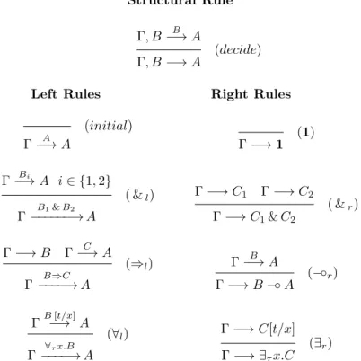
Proof rules for L. A proof system for L is shown in Figure 1. The proof rules result from specializing the proof rules of the system Forum [20]. Forum is a complete presentation of linear logic built around a subset of the linear connectives. In [20],
Structural Rule Γ, B−→ AB Γ, B −→ A
(decide)
Left Rules Right Rules
Γ−→ AA (initial) Γ −→ 1 (1) Γ Bi −→ A i ∈ {1, 2} Γ −−−−−−→ AB1& B2 ( &l) Γ −→ C1 Γ −→ C2 Γ −→ C1& C2 ( &r) Γ −→ B Γ−→ AC Γ −−−−→ AB⇒C (⇒l) Γ B −→ A Γ −→ B −◦ A (−◦r) ΓB [t/x]−→ A Γ−−−−→ A∀τx.B (∀l) Γ −→ C[t/x] Γ −→ ∃τx.C (∃r)
Proviso: in (∀l) and (∃r), t : τ is a closed L-term of type τ . A denotes an atomic formula.
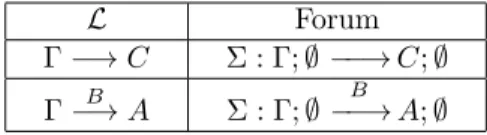
L Forum Γ −→ C Σ : Γ; ∅ −−→ C; ∅ Γ−→ AB Σ : Γ; ∅−−→ A; ∅B
Figure 2: ΠL versus Forum sequents for a given Σ
.
Dale Miller defined a multi-conclusion sequent calculus for this logic, where proofs are uniform by construction. Sequents in this calculus have the form2:
Σ : Γ; ∆ −−→ Ω; Υ and Σ : Γ; ∆−−→ A; Υ,B
where Σ is a signature, Γ and Υ (the unbounded parts of the contexts) are sets of formulas, ∆ (the bounded part of the context) is a multiset of formulas, Ω is a list of (atomic and non-atomic) formulas, A a list of atomic formulas, and B is a formula. All formulas are over the signature Σ.
The correspondence between sequents in the system ΠL and Forum sequents is
established as shown in Figure 2. Since the signature for L is fixed ahead, and we do not have a (∀r) rule, we omit explicit references to Σ in the sequents and proof rules
of ΠL. To ease the notation, we will henceforth use a corresponding abbreviation for
Forum sequents as well.
In other words, our sequents are single-conclusion Forum sequents with empty or singleton bounded context on the left-hand side. The rules (initial) and (decide) correspond respectively to the rules (initial1) and (decideΓ) in Forum. The constant
1 can be defined using the equivalence 1 ≡ ⊥ −◦ ⊥ and the rule (1) can be derived in Forum by (−◦r), (⊥r) and (⊥l). The Forum rules for the exponential ?, and for the
connectives... . . . . . . . . . . . . . ... . .
..., > and ⊥, as well as the rules (∀
r), (−◦l), (⇒r), (initial2), (decide∆)
and (decide?) do not have any corresponding rule in our system. Also note that, as in Forum, the right rules of the system are those for sequents of the form Γ −→ C. On the other hand, the left rules are focussed on (i.e., they are applied only to) the formula B that labels the sequent arrow in Γ−→ A, with A an atomic formula.B
When the formulas in Γ are closed D-formulas, B is a closed D-formula, C is a closed G-formula, and A is a closed atomic formula, we say that the sequents Γ −→ C and Γ−→ A are L-sequents. A proof of an L-sequent that uses the proof rules ofB Figure 1 is said to be an L-proof.
An inspection of the proof rules of system ΠL shows that the left rules are only
applicable to sequents whose succedent is an atomic formula (cf. Figure 1): hence L-proofs are uniform by construction. In the next section we show that L-proofs are complete with respect to provability of L-sequents in higher-order linear logic.
3
Completeness of L-proofs
The completeness result we wish to prove may be stated precisely as follows:
2Sequents in Forum have, in fact, a more general structure. However, Forum proofs involve
every L-sequent has a proof in higher-order linear logic if and only if it has an L-proof.
There is one main restriction in L-proofs with respect to proofs in higher-order linear logic, namely that the substitution terms used in proofs are required to be L-terms. As we already noted, the definition of D-formulas guarantees that the use of D-formulas (i.e., L-terms of type o) as substitution terms for variables of type o preserves the structure of D-formulas, and hence of L-sequents, along an L-proof. Instead, the substitution terms introduced along a proof in higher-order linear logic can be any λ-terms, not necessarily L-terms. Thus, in particular, terms substituted for variables of type o can be formulas other than D-formulas: consequently, the sequents arising in the proof of an L-sequent may happen not to be L-sequents. To prove completeness, we need to show that every such term may be systematically “L-normalized”, i.e., replaced by a corresponding L-term, so that the resulting proof is, in fact, an L-proof.
The idea may be described as follows: given an L-sequent, call Ξ a proof (in higher-order linear logic) for this sequent. The “L-normalization” of Ξ is accomplished in two steps. First we isolate the “sub-proof” of Ξ that has the structure of an L-proof; then we show that every sequent in this sub-proof may be L-normalized, and the sub-proof completed, to produce the desired L-proof.
In the completeness proof we use Forum [20] as logic as reference: this choice does not involve any loss of generality, as it was shown in [20] that provability in Forum is the same as provability in higher-order linear logic. To ease the presentation, we shall use the derived Forum axiom (1), defined as Γ; ∅ −→ 1; Υ in place of the Forum proof of the equivalent formula ⊥ −◦ ⊥. Also, to avoid possible ambiguities, we shall distinguish λ-terms from L-terms using capital letters such as M and N to denote λ-terms, and lower-case letters like t and s to denote L-terms. As for L-terms, α-convertible λ-terms are identified, and we write M ≡ N to state that M and N are identical terms; instead, we write M =βN when M and N are β-convertible. A final
remark on quantifiers is in order. As we noted (footnote 1, page 4) our encoding of quantifiers differs from the standard one, adopted in Forum: however, since a bijection clearly exists between the two encodings, in the rest of this section we will identify the two formulas ∀σx.F and (Πσλx.F ), and similarly the two formulas ∃σx.F and
(Σσλx.F ).
3.1
L-slices
The notion of “sub-proof” is made precise with the definition of L-slice, given below. Before that, we introduce the following class of D-formulas, a generalization of the D-formulas defined in Section 2.
Definition 2 (D-Formulas) We say that a formula F is a D-formula if and only if either one of the following conditions hold: (i) F is a D-formula; (ii) there exists a D-formula ∀τx.H, and F is the formula H[M/x] that results from substituting
any closed λ-term in normal form M for every free occurrence x in H; (iii) F is a conjunction of D-formulas.
The set of D-formulas can be characterized, equivalently, as the set of formulas gen-erated by the following productions:
D ::= A | G ⇒ A | D & D | ∀τV.D
G ::= 1 | A | B −◦ A | G & G | ∃τV.G.
Here A denotes any rigid atomic formula of the form (h t1 . . . tn) where h is a
nonlogical symbol and the ti’s are arbitrary λ-terms (not necessarily L-terms), and
B denotes arbitrary Forum formulas.
Definition 3 (L-slice) Let Ξ be a Forum proof of an L-sequent S. We define the L-slice of Ξ, denoted by ςL(Ξ), to be the partial proof-tree that results from dropping
the subproofs of all the sequents Γ; ∆ −→ A, B −◦ C, Ω; Υ occurring in Ξ, whenever the formula B is not a (closed) D-formula.
The definition of L-slice motivates the introduction of the class of D-formulas: in fact, it is easily seen that the formulas in the antecedent of the sequents of ςL(Ξ) are
closed D-formulas, whereas the formulas in the succedent are closed G-formulas. We next prove a few lemmas that provide a more precise characterization of the structure of L-slices of Forum proofs for L-sequents. We first introduce a new class of sequents, and then give the desired results.
Definition 4 (L-sequents) We say that a Forum sequent is an L-sequent if it has one of the following forms: Γ; D −→ A; ∅, Γ; ∅ −→ G; ∅, or Γ; ∅−→ A; ∅, where Γ isD a set of closed D-formulas, D is a closed D-formula, G is a closed G-formula, and A is a closed A-formula.
L-sequents generalize L-sequents in a way similar to how D and G-formulas generalize D and G-formulas. What we show next is that if we take a Forum proof of an L-sequent, then every sequent in the L-slice of the proof is, in fact, an L-sequent. We first need the following auxiliary result.
Lemma 5 Let Γ be a set of closed D-formulas, D be a closed D-formula, G a closed G-formula, A a closed A-formula, and ∆ a multiset of closed D-formulas. Then we have:
· if the sequent Γ; ∆ −→ A; ∅ is provable in Forum, then ∆ must be the emptyD multiset;
· if the sequent Γ; ∆ −→ A; ∅ is provable in Forum, and ∆ is non empty, then ∆ must be a singleton.
Proof By a straightforward induction on the structure of the Forum proof.
Lemma 6 Let S be an L-sequent, and Ξ be a Forum proof of S. Then, every sequent in ςL(Ξ) is an L-sequent.
Proof The proof is by induction on the height of Ξ. The claim is clearly true when Ξ has height 1, as in this case S must be an axiom (initial1) of the form Γ; ∅
A
−→ A; ∅, or an axiom (1) of the form Γ; ∅ −→ 1; ∅. Then, assume that the claim holds for all
proofs (of L-sequents) of height less than h, and consider a Forum proof Ξ of height h. The proof is now by a case analysis on the last rule used in Ξ. Most cases are vacuous since the rule could not have been applied to S, S being an L-sequent. Below we give the most interesting cases.
· (−◦r). Since S is an L-sequent, it must be of the form Γ; ∅ −→ B −◦ A; ∅.
We distinguish two subcases, depending on the structure of B. If B is not a D-formula, the thesis follows immediately, as the sequent is a leaf of ςL(Ξ). If, instead, B is a D-formula, the premise of the rule is the sequent Γ; B −→ A; ∅, which is an L-sequent. The thesis follows then from the induction hypothesis. · (decideΓ) The claim follows directly from the induction hypothesis, as the
se-quent in question may only be of the form Γ; ∅ −→ A; ∅. The other case, when the sequent in question is Γ; D −→ A; ∅, is vacuous. To see why, note that the upper sequent of the rule would be the sequent Γ; D D
0
−→ A; ∅ for some D0 in Γ.
By Lemma 5, we know that the latter sequent is not provable in Forum: hence Ξ would not be a Forum proof, a contradiction.
· (decide∆) The sequent in question is again Γ; D −→ A; ∅ and the premise of the
rule is Γ; ∅−→ A; ∅, an L-sequent. The claim follows then from the inductionD hypothesis.
With the above proof, we implicitly have proved the following result.
Corollary 7 Let Ξ be a Forum proof of an L-sequent. Then, every instance of (−◦r) occurring in ςL(Ξ) and focusing on the formula D, always occurs just below an
instance of (decide∆) with D as principal formula.
In other words, all the derivation schemes of the form Γ; ∅−→ A; ∅D
Γ; D −→ A; ∅
(decide∆)
Γ; ∅ −→ D −◦ A; ∅ (−◦r)
occurring in an L-slice can be coalesced and replaced by an application of the (−◦r) of
system ΠL(cf. Section 2, Figure 1). As a consequence, we may simplify the definition
of L-sequents to comprise only sequents in the forms Γ; ∅ −→ G; ∅ or Γ; ∅−→ A; ∅.D Given this observation, we will further simplify the notation of L-sequents and use the following presentation:
Γ −→ G for Γ; ∅ −→ G; ∅, Γ−→ AD for Γ; ∅−→ A; ∅.D
A final lemma establishes the relations between the D and G-formulas occurring in an L-slice, and their corresponding D and G-formulas.
Lemma 8 Let S be an L-sequent, Ξ be a Forum proof of S, and let Γ −→ G and Γ−→ A be L-sequents in the L-slice ςD L(Ξ). Then:
· every formula in Γ ∪ {D} may be written as D[M1/x1] . . . [Mn/xn], where D is
a D-formula that has the same top-level connective as the formula in question, the variables x1, . . . , xnare free in D, and the Mi’s are closed λ-terms in normal
form;
· the formula G (respectively A) may be written as G[N1/y1] . . . [Nm/ym] (resp.
A[N1/y1]...[Nm/ym]) where G (resp. A) is a G-formula that has the same
top-level connective as G (resp. A), the variables y1, . . . , ymare free in G (resp. A),
and the Ni’s are closed λ-terms in normal form.
Proof The proof is by induction on the height h of the L-slice. In order for induction to work, we prove a slightly more general result, where S is an L-sequent, rather than an L-sequent. The lemma follows then immediately, noting that L-sequents are also L-sequents (this follows immediately by definition of D- and G-formulas).
The base of induction, when h = 1, follows immediately: the only nontrivial case is when S is the sequent Γ −→ B −◦ A, which can be written as (x −◦ A)[. . . , B/x, . . .] for some atomic formula A (note that B is a closed non-D-formula).
When h > 1, the proof is a case analysis on the last Forum rule in the slice. Most cases are vacuous, as S is an L-sequent and the rule could not have been applied to S; the non-vacuous cases follow directly by induction hypothesis on the upper sequents of the rule, which are easily verified to be L-sequents, when the lower sequent is itself an L-sequent.
Having formalized the notion of “sub-proof” we move on to the next step of our con-struction. As we anticipated, the idea is to “L-normalize” every “wrong” term arising in the proof, i.e., replace that term with a corresponding L-term. The argument we use is constructive, and relies on essentially the same idea used in the completeness proof for the language of higher-order hereditary Harrop formulas (hohh) of [21]. As in that case, there are two cases to consider, depending on whether the “wrong” term is substituted for a variable that occurs in the scope of a non-logical or logical constant. In the first case the solution is simple because the wrong term may be L-normalized to any L-term of type o. In the second case, since we are restricting attention to L-slices, the “wrong” term must be a formula occurring to the left of a linear implication, as B in B −◦ A, with B −◦ A resulting from substituting a variable Dv-formula in the antecedent of a G-formula Dv −◦ A. Now, it would seem natural to L-normalize B −◦ A to the tautological formula ν(A) −◦ ν(A), where ν(A) is the L-normalization of A. However, a problem with this simple L-normalization scheme arises in situations where the same substitution term is used in different sequents along the L-slice.
Consider the following L-slice of a derivation, where φ : o is not a D-formula, and where Γ contains the following D-formulas:
D1= ∀v. ((v −◦ p(v)) & p(v)) ⇒ q | {z } D0 1 ; D2= ∀w. ((w −◦ r(w))) ⇒ p(w) | {z } D0 2 .
Γ −→ (v −◦ p(v))[φ/v] (−◦r) Ξ0 Γ −→ (v −◦ p(v)) & p(v)[φ/v] ( &r) Γ−→ qq (initial) Γ D10[φ/v] −−−−−−→ q (⇒l) Γ −→ q (decide + ∀l)
Here Ξ0 is the following proof:
Γ −→ (w −◦ r(w))[φ/w] (−◦r) Γ p(w)[φ/w] −−−−−−−→ p(v)[φ/v] (initial) Γ D20[φ/w] −−−−−−→ p(v)[φ/v] (∀l) Γ −→ p(v)[φ/v] (decide) + (∀l)
We assume that Γ−→ p(φ) and Γφ −→ r(φ) have Forum proofs. Now, if we used theφ naive L-normalization we outlined above, we would end up with two L-normalizing terms for φ, namely: p(ν(φ)) and r(ν(φ)) where ν(φ) denotes any L-term of type o. Clearly, then, the result of L-normalization would not be a proof, for what we actually need is the L-term p(ν(φ)) & r(ν(φ)). Below, we give a technique for systematically computing L-normalization terms for any given L-slice. The technique generalizes the idea we just illustrated yielding L-normalization terms in the form of (conjoined) universally quantified D-formulas.
3.2
Computing L-Normalization Terms
As illustrated by the previous example, L-normalization terms may not, generally, be determined by simply looking at the sequent where they are required: a global inspection of the L-slice is needed to find the appropriate D-formula for every “wrong” witness of type o in the original proof. However, what we can do, locally to every sequent, is to collect the L-normalizing terms for every potentially “wrong” witness that might be introduced by a substitution over a variable of type o. This is the idea behind the following definition.
Definition 9 (Local L-Normalization) We say that a variable v has a formula occurrence in a formula F if and only if v has at least one occurrence in F that is not in the scope of a non-logical constant. Let F be a D or G-formula, let B denote any formula, and let v be a variable. The local L-normalization terms for v in F, written N[v, F] is defined inductively as follows:
N[v, F1& F2] = N[v, F1] ∪ N[v, F2];
N[v, ∀τx.D] = N[v, D];
N[v, ∃τx.G] = N[v, G];
N[v, B−◦A] = {A} ∪ N[v, B] if v has a formula occurrence in B, N[v, B−◦A] = N[v, B], otherwise;
N[v, B] = ∅ if none of the above applies. To exemplify, we have N[v, D0
1] = {p(v)} and N[w, D20] = {r(w)} in the formulas of
the previous derivation.
Given the L-slice of a Forum proof, we may compute the L-normalization term of type o by “decorating” each sequent in the slice with a set N of local L-normalization terms. Where N | Γ −→ G denotes a decorated sequent, this process can be accomplished in the following manner:
· the set N at the leaves of the slice is empty;
· for every instance of a rule with two premises, the set N at the lower sequent is the union of the corresponding sets at the upper sequents;
· for every instance of a rule with one premise, with the exception of the (∀l) and
(∃r) rules, the set N attached to the upper sequent is simply “copied” in the
lower sequent;
· for every instance of (∀l) the set N is computed as follows:
N | Γ−−−−→ AD[t/x]
N ∪ N[x, D] | Γ−−−−→ A∀ox.D (∀l)
· for every instance of (∃r) the set N is computed as follows:
N | Γ −→ G[t/x] N ∪ N[x, G] | Γ −→ ∃ox.G
(∃r)
Proceeding in this way at every sequent of the L-slice, the set N occurring at the root of the L-slice can be characterized as follows.
Lemma 10 Let Ξ be a Forum proof of an L-sequent Γ −→ G, and let N be the decoration associated to the root of ςL(Ξ) by the process just described. Then, for every A such that Γ −→ B −◦ A is a leaf sequent of ςL(Ξ), it is the case that A ∈ N . Proof By construction, noting that, by the definition of G-formulas, B corresponds to the formula v[t1/x1, . . . , B/v, tn/xn], for some variable v : o.
Definition 11 (Canonical L-Normalization Terms) We introduce a canonical L-normalization term at each sort. For sorts other than o choose any distinguished constant of that sort as the normalization term, and denote it with νσ. For the sort
o, L-normalization terms are defined as follows. Let ςL be an L-slice, and let N be
the decoration computed at the root of ςL by decorating each sequent in ςL in the
manner described above. The canonical L-normalization term of type o, denoted by νo, is defined as follows:
· if N = {A1, . . . , An}, and Ai = (hiM1. . . Mk), then νo = A∀1& · · · & A∀n,
where A∀i = ∀τ1x1. . . . ∀τnxk.(hix1. . . xk).
· If N = ∅, then νo= co, where cois any constant symbol of type o in Σ.
When N 6= ∅, the definition of νo formalizes the idea we already described. When
N = ∅, all the λ-terms to be L-normalized in the slice occur nested within a non-logical constant: in this case, any choice of νo serves our purposes. The notion
of L-normalization terms is well defined, given our initial assumption that all sorts (including o) are nonempty. It only remains, now, to define the L-normalization mapping that transforms every formula into a corresponding D-formula (preserving L-terms and D-formulas).
The normalization mapping is defined over the class of λ-terms that arise from substituting normal-form λ-terms for variables of the L-terms occurring in the L-slice of a Forum proof.
Definition 12 (L-Normalization) Let Ξ be a Forum proof, σ be a sort, and let M : σ be a λ-term in normal form occurring in ςL(Ξ). The L-normalization of M in ςL(Ξ), written ν(M ), is defined inductively as follows:
· if M : σ is a typed constant or a variable, then ν(M ) = M ;
· if M : σ is the term (M0M1. . . Mn), then distinguish the following three
sub-cases:
− if M0: σ1× · · · × σn → σ is a nonlogical constant, and Mi : σi for i = 1..n,
then ν(M ) = (M0ν(M1) . . . ν(Mn));
− if M0 is a logical constant, and M is a D-formula, then ν(M ) = ν−(M )
where ν− is the mapping defined by the following mutual recursion:
ν−(A) = ν(A) ν−(G ⇒ A) = ν+(G) ⇒ ν(A) ν−(D & D) = ν−(D) & ν−(D) ν−(∀τv.D) = ∀τv.ν−(D) ν+(1) = 1 ν+(A) = ν(A) ν+(B −◦ A) = ν(B) −◦ ν(A) ν+(G & G) = ν+(G) & ν+(G) ν+(∃ τv.G) = ∃τv.ν+(G) − ν(M ) = νσ otherwise.
Remarks The definition of L-normalization is given without explicit treatment of λ-abstraction: this is consistent with the intended domain of the normalization mapping. In fact, as λ-terms are substituted in L-terms for variables of basic types, they may not be λ-abstractions; furthermore, since substitution terms are assumed to be in normal form, λ-abstractions may only occur within substitution terms in the argument position of a λ-normal application subterm: all such occurrences are normalized away by the last clause of the definition of L-normalization.
The normalization mapping satisfies some important properties: it preserves equa-lity over the class of terms of interest, and it commutes with substitution of λ-terms into L-terms. As a reminder, we recall that equality over simply-typed λ-terms is β-convertibility, denoted by =β. When restricting to λ-terms in normal form (or to
L-terms) equality reduces to α-convertibility, hence to syntactical identity, as we work modulo renaming of bound variables.
Lemma 13 Let σ be a sort, and M, N : σ be two λ-terms in normal form. Then ν(M ) ≡ ν(N ) whenever M ≡ N .
Proof Immediate, since the normalization mapping ν does not depend on the names of bound variables: hence it maps α-convertible λ-terms into α-convertible L-terms. Also note that the result holds when M and N are L-terms, as L-terms are also λ terms in normal form.
Lemma 14 Let M be a closed λ term in normal form, and let t be any L-term with x free in t, and M free for x in t. Then ν(t[M/x]) ≡ t[ν(M )/x], and t[ν(M )/x] is itself an L-term.
Proof The proof is by induction on the structure of t. We note, however, that not every subterm of a given L-term is itself an L-term. Hence, in order for induction to work, we prove the following, more general, result.
1. if t : σ is an atomic L-term then ν(t[M/x]) ≡ t[ν(M )/x], and t[ν(M )/x] is an L-term;
2. if t : o is a D-formula, then ν−(t[M/x]) ≡ t[ν(M )/x], and t[ν(M )/x] is a D-formula;
3. if t : o is a G-formula, then ν+(t[M/x]) ≡ t[ν(M )/x], and t[ν(M )/x] is a
G-formula.
The proof is by induction on the structure of t, simultaneously for (1), (2) and (3). 1. · If t is a variable or a constant, the claim follows directly from the definition
of normalization (cf. Definition 12).
· If t ≡ (h t1. . . tn) : σ, then ν((h t1. . . tn)[M/x]) ≡ ν(h t1[M/x] . . . tn[M/x])
and the latter is equal to (h ν(t1[M/x]) . . . ν(tn[M/x])) by definition. Then
the proof follows from the induction hypothesis (1) or (2) depending on the structure of the ti’s.
2. If t is atomic the proof follows exactly as in the second subcase above. In all the remaining cases, the thesis follows from the induction hypothesis (1), (2) or (3).
3. If t ≡ 1 the claim follows immediately. If t is atomic the claim follows exactly as in case (2) above. In all the induction cases the thesis follows from the induction hypothesis (1), (2) or (3).
Lemma 15 Let t, s be two L-terms with x free in t and y free in s, and M, N two closed λ-terms in normal form such that M is free for x in t and N is free for y in s. Then, t[ν(M )/x] =β s[ν(N )/y] whenever t[M/x] =βs[N/y].
Proof Since M and N are assumed to be in normal form, and substitution of terms of basic types in L-terms does not produce β-redexes, one has that t[M/x] =βs[N/y]
if and only if t[M/x] ≡ s[N/y]. Now, by lemma 13 and by lemma 14, it follows that t[ν(M )/x] ≡ ν(t[M/x]) ≡ ν(s[N/y]) ≡ s[ν(N )/y].
As a consequence, the following property holds.
Lemma 16 Let D, D0 be two D-formulas, and M1, . . . , Mn, N1, . . . , Nk be closed
λ-terms in normal form. If D[M1/x1] . . . [Mn/xn] =β D0[N1/y1] . . . [Nk/yk], then
D[ν(M1)/x1] . . . [ν(Mn)/xn] =βD0[ν(N1)/y1] . . . [ν(Nk)/yk].
Proof Observe that D[ν(M1)/x1] . . . [ν(Mn)/xn] ≡ D[ν(M1)/x1, . . . , ν(Mn)/xn], as
substitutions of closed λ terms in normal form for variables of basic types do not compose. Then the proof follows from Lemma 15 by induction on n.
We may now prove the desired completeness result.
Theorem 17 (Completeness vs Forum) Given an L-sequent of the form Γ −→ G, this sequent has a proof in Forum if and only if it has an L-proof.
Proof The “only if” part of the proof is trivial, as L-proofs are, in fact, Forum proofs. For the “if” part, we reason as follows.
Given Ξ, the Forum proof of the sequent, consider the L-slice of Ξ: from Lemma 6, we know that sequents in the L-slice have either the form Γ −→ G, or Γ−→ A,D where D is a D-formula, G is a G-formula, and A is an A-formula. Given any formula F ≡ F [M1/x1] . . . [Mn/xn], let now bF denote the formula F [ν(M1)/x1] . . . [ν(Mn)/xn].
We show that for every sequent of the form Γ −→ G or Γ−→ A of the L-slice anD L-proof exists for the sequent Γ −→ bG and Γ −→ bDb A, respectively. The theorem follows then easily from this claim. The proof of the claim is by induction on height of the subderivation rooted at the sequent in question.
Base Case. If the subderivation has height 1, then the sequent in question either (1) or (initial). In the former case the claim immediately follows. In the latter case, from Lemma 8, we know that it may be written as
Γ
A[M1/x1]...[Mn/xn]
−−−−−−−−−−−−−−−→ A0[N
1/y1] . . . [Nm/ym],
with A[M1/x1] . . . [Mn/xn] =β A0[N1/y1] . . . [Nm/ym]. By Lemma 16, this implies
that also A[ν(M1)/x1] . . . [ν(Mn)/xn] =β A0[ν(N1)/y1] . . . [ν(Nm)/ym]. Thus, the
se-quent
Γ
A[ν(M1)/x1]...[ν(Mn)/xn]
−−−−−−−−−−−−−−−−−−−→ A0[ν(N
1)/y1] . . . [ν(Nm)/ym]
is initial, and hence derivable.
Induction Cases. By a case analysis on the last rule of the subderivation Ξ. We first consider the cases of the left rules. Let Γ−→ A be the sequent in question:D
· (&l). In this case D = D[M1/x1]. . .[Mn/xn] = D1& D2, for some formulas D1
and D2. From Lemma 8 we know that D is a D-formula of the form D01& D02,
for suitable D01 and D20, which implies that the Di’s, (for i = 1, 2), are of
two formulas D0i; from the induction hypothesis, it then follows that the two sequents Γ D0 i[ν(M1)/x1]...[ν(Mn)/xn] −−−−−−−−−−−−−−−−−−−−→ bA,
(for i = 1, 2) have an L-proof. An application of (&l) yields now the desired
L-proof for
Γ
D[ν(M1)/x1]...[ν(Mn)/xn]
−−−−−−−−−−−−−−−−−−−→ bA.
· The same reasoning applies to the remaining left rules: the cases (⊥l), (−◦l) and
(... . . . . . . . . . . . . . ... . . ...
l) follow vacuously because none of these rules could have been applied, given
the hypothesis on the structure of D. We give the case of (∀l) as representative
of the remaining possible cases. In this case D[M1/x1]. . .[Mn/xn] is of the form
∀x.D0[M
1/x1] . . . [Mn/xn] for some D-formula D0, and the premise of the rule
is the sequent
Γ
D0[M
1/x1]...[Mn/xn][t/x]
−−−−−−−−−−−−−−−−−−−→ A,
for some closed λ-term t in normal form. From the induction hypothesis, we know that
Γ
D0[ν(M1)/x1]...[ν(Mn)/xn][ν(t)/x]
−−−−−−−−−−−−−−−−−−−−−−−−−−→ bA
has an L-proof, and the L-proof for the desired sequent may be obtained by an application of (∀l) on the last sequent.
Next we consider the right rules. Most cases are vacuous, for the rule could not have been applied to the sequent in question. The case of (∃r) is similar to the case
of (∀l) we just considered. The cases (&r) and (decideΓ) follow from the induction
hypothesis. The case of (−◦r) is worked out below.
Assume that the sequent is Γ −→ B −◦ A, derived by (−◦r). ¿From Lemma 8, we
know that B −◦ A may be written as (D −◦ A)[N1/y1] . . . [Nm/ym] for some G-formula
D −◦ A. Now we distinguish the following cases, depending on the structure of D. · If D is a D-formula, the claim follows from the induction hypothesis, for
(D −◦ A)[N1/y1] . . . [Nm/ym] = D[N1/y1] . . . [Nm/ym] −◦ A[N1/y1] . . . [Nm/ym],
and the upper sequent of the rule is the sequent
Γ −−−−−−−−−−−−−−−→ A[ND[N1/y1]...[Nm/ym] 1/y1] . . . [Nm/ym],
derivable by hypothesis.
· If, instead, D is not a D-formula, then it must be either a variable, or a conjunc-tion of Dv-formulas. The first case is worked out next, the second is similar. Given that D[N1/y1] . . . [Nm/ym] is closed, if D is a variable it must be the case
that D = yi, for some i = 1, . . . , m, and D[N1/y1] . . . [Nm/ym] = Ni. Now, we
have two possible subcases: (i) either there exists a D-formula D0, and closed terms Ni0, and variables yi0 free in D0 such that D0[N10/y01] . . . [Nk0/yk0] = Ni, or
(ii) no such D0 exists. In the first subcase the claim follows from the induction hypothesis, for
D[Ni/yi] . . . [Nm/ym] −◦ A[N1/y1] . . . [Nm/ym]
may be written as
D0[N10/y10] . . . [Nk0/y0k] −◦ A[N1/y1] . . . [Nm/ym],
and we can apply the induction hypothesis on the premise of the rule. In the second subcase, the sequent Γ −→ B −◦ A must be a leaf-sequent in the L-slice. ¿From Lemma 10 it follows that A ∈ N , where N is the decoration occurring at the root of the L-slice. Letting A = (h M1. . . Mk), from Definition 11, we
have that
νo= A∀1. . . & ∀τ1x1. . . . ∀τkxk.h(x1, . . . , xk) & . . . A
∀ n,
for some A∀1, . . . , A∀n. Finally, since by definition, it holds that
ν(B −◦ A) = νo−◦ (h ν(M1) . . . ν(Mk)),
an L-proof for Γ −→ ν(B −◦ A) can be formed as shown below:
Γ (h x1... xk)[ν(M1)/x1]...[ν(Mk)/xk] −−−−−−−−−−−−−−−−−−−−−−−−−−→ (h ν(M1) . . . ν(Mk)) (initial) .. .. k (∀l) steps Γ−−−−−−−−−−−−−−−−→ (h ν(M∀x1....∀xk.(h x1... xk) 1) . . . ν(Mk)) .. .. n (&l) steps Γ νo −→ (h ν(M1) . . . ν(Mk))
4
A Calculus of Objects
In this section we describe the syntax and the semantics of Ob−◦, an untyped
object-based language that has all the essential ingredients of the object calculi we wish to characterize. The syntax of Ob−◦ resembles the syntax of the untyped calculus of [2].
Unlike [2], however, we use a logic-programming style for the syntax of methods, so that methods may be written as formulas.
Objects
o ::= s, x, y, . . . variables
| obj[ ] the empty object
| o.m := ∀s m method addition/override
Method Definitions
m ::= a 7→ o if b conditional definition
| ∀x m quantified definition Method Bodies
b ::= o.m a 7→ o message send
| b, b conjunction
Argument List
a ::= (o1, . . . , on) n ≥ 0 arguments
Objects are formed as the result of a sequence of updates, starting from the empty object. An object update is written o.m := ∀s m, and represents the object obtained by either replacing the current method definition for the label m in o with the new definition ∀s m, or by adding a new label m and associated definition. In either case the semantics of update is functional: first it produces a copy of the object being updated, and then updates (or extends) the copy. The object containing a given method is called the object’s host object, and the quantified variable s represents the self-parameter for the method, to be bound to the host object upon invocation of that method (see below).
Method definitions have the form of clauses, where the head a 7→ o defines the correspondence between the input arguments a and the result o, and the body defines the conditions to be satisfied for this correspondence to hold. Method definitions may contain free variables, as long as each of these variables occur in the scope of a quantifier in the surrounding context. This generality, which is required to express objects and methods with “nested” occurrences of “self” (see Example 21) also justifies the explicit use of quantifiers in the syntax of methods.
Method bodies are formed as conjunctions of method invocations (message sends) of the form o1.m A 7→ o2 whose intended semantics is as follows. Assume that the
definition for m in o1 is ∀s m: to evaluate o1.m A 7→ o2, evaluate m[o1/s], i.e., the
method definition with the object o1 bound to the self-parameter, using arguments
A and expecting o2as a result.
Remarks. In the above productions we assume that the method labels m are chosen from a denumerable set of method labels M, and that there are denumerably many names for variables.
Primitives for object extension are not available in the calculus of [2], whereas they are provided as a separate extension operator (different from the overriding operator) in [7]. An equivalent, extensional, presentation of objects could be adopted, where objects are defined as collections obj[m1 = ∀s m1, . . . , mn = ∀s mn] of components
mi = ∀s Mi, with distinct labels mi ∈ M, and associated method definitions mi,
for i ∈ 1..n. The two views (i.e., the intentional view we have adopted, and the extensional one) could be unified by defining an equational theory over objects based on the following two axioms (the notation obj[mi= ∀s mi]i∈1..nis short for obj[m1=
∀s m1, . . . , mn= ∀s mn]):
(Eq-Override) (j ∈ 1..n)
(obj[mi= ∀s mi]i∈1..n.mj := ∀s m) = (obj[mj= ∀s m, mi= ∀s mi]i∈1..n,i6=j)
(Eq-Extend) (j 6∈ 1..n)
Similar axioms are used in the equational theory of [2], and in the extended calculus studied in []. While defining an equational theory based on the above axioms would not be conceptually problematic, it is of no interest in the context of the present paper.
4.1
A Proof System
Unlike [2], where the semantics of the calculus is defined by reduction, evaluation in Ob−◦ is a process of proof search, that we formalize in a natural semantics style with
a set of inference rules. A goal, or query, is an existentially quantified conjunction of message sends:
Query Q ::= b | ∃x.Q
Below we give a proof system for Ob−◦, together with a few examples that should
help clarify how the evaluation works.
In defining the proof rules, a mechanism is needed for extracting the method definitions that reside within objects. The following function serves this purpose.
· select(m, (o.m := ∀s m)) = ∀s m;
· select(n, (o.m := ∀s m)) = select(n, o) if n 6= m;
As we said, a goal in Ob−◦ is a conjunction of message sends: since all the methods
needed to handle the message reside within the receiver of that message, no “program” is really needed to evaluate a goal. Given the select function defined above, the proof rules can be formalized as follows:
` [o/x]Q (o closed) ` ∃x.Q (exist) ` b1 ` b2 ` b1, b2 (and) a 7→ o ∈ hmi m ` a 7→ o (initial) m[o1/s] ` a 7→ o2 select(m, o1) = ∀s m ` o1.m a 7→ o2 (send) ` b a 7→ o if b ∈ hmi m ` a 7→ o (backchain)
These rules define evaluation in terms of two mutually recursive relations of provabi-lity: a principal, unary, relation that evaluates messages (and conjunctions thereof), and a subsidiary, binary, relation that accounts for the backchaining steps needed to evaluate a method definition. The notation hmi in the (backchain) and (initial) rules indicates the set of closed instances of m, i.e., the smallest set that satisfies the following conditions:
m ∈ hmi;
∀x m0 ∈ hmi =⇒ m0[o/x] ∈ hmi for every closed object o.
As a further remark, we note that the notion of provability we refer to here is strictly operational. In Section 5 we will show that this operational characterization has an equivalent formulation in terms of the notion of L-provability.
4.2
Examples
When instrumented with a unification algorithm for computing bindings for the logical (i.e., existentially quantified) variables of a query, the rules given above can be directly employed as the core of an interpreter. In presenting the examples we use logical variables, (denoted by capital letters) instead of existentially quantified variables in queries, and we make implicit appeal to the existence of such unification algorithm (see Section 6 for further discussion).
The following shorthands are used in the example to ease readability. We write obj[m1 = ∀s m1, . . . , mn = ∀s mn] to denote the object that results from the
se-quence of extensions (. . . (obj[ ].m1:= ∀s m1) . . .).mn:= ∀s mn. Also, we omit empty
argument lists and write “ 7→ o” instead of “() 7→ o”
Example 18 (Diagonal points) The first example represents a two-dimensional diagonal point with two fields, x, and y. In Ob−◦, this object can be expressed as
follows:
d 4= obj[x = ∀s 7→ 1, y = ∀s ∀v ( 7→ v if s.x 7→ v)].
Both fields are encoded as methods: the x field is constant (it does not depend on the self variable s) whereas y is a “true” method, which does depend of the self variable. Given a logical variable V , consider evaluating the query d.x 7→ V . The evaluation takes two steps: a (send) step selects the definition of the method definition for x, and unifies the head of the definition with 7→ V , producing the substitution [1/V ]. A subsequent (initial) step terminates the process, and returns the substitution [1/V ] as result.
A similar sequence of steps is used to evaluate the query d.y 7→ V . After the first (send) step, a (backchain) step leads to evaluating the body of the y method; this is just the message d.x 7→ V , which is evaluated as before. The result is again the substitution [1/V ].
Example 19 (One-dimensional point) The second example is a one-dimensional point with a “move” method. This object can be represented as follows:
pt 4= obj[x = ∀s 7→ 3, mv = ∀s1mmv[s1]],
where
mmv[s1] 4
= ∀x, y ((y) 7→ (s1.x := ∀s2 7→ x+y) if s1.x 7→ x).
Consider the message send pt.mv(2) 7→ P . As in the previous example, we first se-lect the definition associated with mv, perform the self-substitution mmv[pt/s1], and
continue evaluating the query (2) 7→ P . Backchaining over mmv[pt/s1], produces the
substitution
[2/y, (pt.x :=∀s1 7→ x+2)/P ].
Evaluating the body of the definition yields then the new substitution [3/x] and, composing the two substitutions, P gets bound to pt.x :=∀s1 7→ 3+2, which is just
the object:
Example 20 (Object-based Inheritance) The next example illustrates method inheritance between objects. Consider again the pt object of the previous example, and let mcol be the definition ∀s 7→ blue. Now, consider the following composite
query:
(pt.col := mcol).move(2) 7→ P, P.col 7→ C.
As in the previous example, evaluating the first message yields the binding [(pt.x :=∀s1 7→ x+2)/P ],
and then the second message returns [blue/C] as expected.
Example 21 (Object numerals) As a further example, we show how natural num-bers can be represented in Ob−◦. Following [2], we define object-numerals as objects
that respond to the methods is zero (test for zero), pred (predecessor) and succ (successor) and behave like natural numbers. In fact, we need only to define the numeral zero as the “prototypical” number, and let all other numerals be generated by repeated applications of the succ method.
obj[is zero = ∀s 7→ true, pred = ∀s 7→ s, succ = ∀s 7→ o[s]] where o[s] is the following object:
o[s] = (s.is zero := (∀s0 7→ f alse)).pred := ∀s0 7→ s.
One easily verifies, with a few tests, that the operational semantics of natural numbers is well represented. In particular, note that the body of succ consists of two cascaded updates for the self-parameter: when invoked on any object-numeral, succ updates the is zero method to answer f alse and updates the pred method to return the current value of self when succ is invoked.
Example 22 (Representing Classes) As a final example we show that classes and class-based inheritance can be represented in a fairly natural way in Ob−◦. The
representation we outline below differs from the record-of-pre-methods model of [1]: instead, it is inspired to that of [8] where object extension is used in an essential way to render the effect of class inheritance. A class is represented as an object like the following:
classA 4
= obj[new = ∀s, argsA(argsA) 7→ obj[. . . , mi= ∀sibody(argsA), . . .]].
classA consists of just one method, the constructor function new: a call to the
con-structor on the class creates an instance by initializing the concon-structor parameters with corresponding arguments passed along with the call. A subclass classBof classA
may then be defined by inheritance as follows, using method addition or override:
classB 4
= obj[new = ∀s, argsAB(argsAB) 7→ (classA.new(argsA)).m := ∀s body(argsB)].
Here m may either be a new method not present in (instances of) classA, or an existing
5
Encoding Ob
−◦in L
In this section we show that L is well suited as a specification language for Ob−◦.
We do this by first defining an encoding function that maps object expressions and queries in Ob−◦into, respectively, L-terms and G-formulas from L; then we show that
the select function as well as the (send) inference rule used in the proof system of Ob−◦ can be axiomatized as an L-theory (i.e., as a set of closed D-formulas). Finally,
we show that evaluating an Ob−◦ query corresponds to finding an L-proof for the
encoding of that query in L.
The intuition behind the encoding is rather straightforward: objects from Ob−◦
are encoded in L as lists of pairs (method label, method definition), while method definitions are encoded as D-formulas from L. Care must be used only to ensure that L-terms of appropriated sorts are chosen to represent object-expressions from Ob−◦.
Since Ob−◦ is untyped, this is easily accomplished by choosing one of the types of L
as the universal type for all the object expressions from Ob−◦: we denote this type
with ω in the following. The details of the encoding are described below: we define it in terms of four mutually recursive functions, one for each syntactic category of Ob−◦.
Encoding of Objects [[ o ]]1: ω.
Choose a type µ as the type of method labels from M. Then:
· choose a type π to represent the type of values built as pairs (m, D) where m is a method label, D is a D-formula in L, and (·, ·) : µ × o → π is a non-logical constant;
· choose a type ω to represent the type of every list of π’s, and two non-logical constants, [ ] : ω and :: π × ω → ω to represents the constructors of lists. Given these choices, the encoding of objects can be defined as follows:
· [[ x ]]1= x;
· [[ obj[ ] ]]1= [ ];
· [[ o.m := ∀s m ]]1= (m, ∀
ωs [[ m ]]2m,s) :: [[ o ]]1
Having chosen ω as the universal type for the terms of Ob−◦, the untyped quantifiers
from Ob−◦ is represented by the typed quantifier ∀ω from L.
Encoding of Method Definitions [[ m ]]2
m,self: o.
As anticipated, method definitions are encoded as D-formulas in L. The encoding function is indexed by a method label and by the self variable to allow a proper encoding of the head of the definition. Again, the untyped quantifiers from Ob−◦
are represented by the typed quantifier ∀ω. The definition uses a further type, α,
to represent the type of arguments (lists of objects), and of a non-logical constant meth : µ × ω × α × ω → o from the signature.
[[ ∀x m ]]2m,self = ∀ωx [[ m ]]2m,self;
[[ a 7→ o if b ]]2m,self = [[ b ]] 3
⇒ meth m self [[ a ]]4 [[ o ]]1 [[ a 7→ o ]]2m,self = meth m self [[ a ]]
4
Encoding Method Bodies. [[ b ]]3: o.
Messages are represented as corresponding atomic formulas from L: the definition uses the non-logical constants send : ω × o → o to construct an atomic formula out of a message send, and msg : µ × α × ω → o to form the message. The comma operator from Ob−◦ is interpreted in L as &.
[[ o.m a 7→ o ]]3 = send [[ o ]]1(msg m [[ a ]]4[[ o ]]1) [[ b1, b2]]3 = [[ b1]]3& [[ b2]]3.
Encoding of Arguments. [[ a ]]4: α.
Arguments are encoded as lists of objects, choosing a type α, and two non-logical constants () : α, and (·, ·) : ω × α → α from the signature.
[[ () ]]4 = ();
[[ (o1, . . . , on) ]]4 = ( [[ o1]]1, [[ o2, . . . , on]]4).
Specification of the operational semantics. We first define the selection D-formulas, used to extract methods from objects. The definition uses the non-logical constant select : ω × µ × o → o from the signature. Given the encoding of objects as lists of pairs (method label, method definitions), the definition should be clear if one thinks of d as the encoding of a method definition.
∀µm. ∀ωo. ∀od. select ((m, d ) :: o) m d.
∀µm. ∀µn. ∀ωo. ∀od. m 6= n & select o m d ⇒ select ((n, ) :: o) m d.
Here m 6= n denotes that the two labels are different. Then we define the evaluation D-formula that renders the effect of self-substitution.
∀µm. ∀ωo1. ∀ωo2. ∀αa.
∃od.(select o1m d & (d −◦ (meth m o1 a o2))) ⇒ send o1(msg m a o2).
It is worth taking the time to show why this captures the intended semantics of method invocation. Let Γeval be the set of evaluation and selection D-formulas we
introduced above; let then obj be the encoding of an object containing a definition for the label m, and let arg be the encoding of a list of arguments. Now consider the following L-sequent:
Γeval −→ ∃ωo.send obj (msg m arg o).
Considering how a (uniform) L-proof could be constructed for this sequent, one easily sees that the self-substitution semantics is rendered correctly. The sequence of proof steps can be described as follows:
1. Apply (∃r) to find a suitable L-term, say val, as a witness for o;
2. Apply (decide) to move the evaluation D-formula in the bounded part of the context; then apply four (∀l) steps to substitute m, obj, arg and val, respectively
3. Apply (⇒l): the right sequent on the premises is initial; the left-sequent is
Γeval−→ ∃od.(select obj m d & (d −◦ (meth m obj arg val))).
4. Now apply (∃r) to find a D-formula dmas substitute for d such that the sequent
Γ −→ select obj m dmis provable, and then consider the sequent
Γ dm
−→ meth m obj arg val,
that results from applying (−◦r) on Γ −→ dm −◦ (meth m obj arg val).
5. It is at this point that the self-substitution takes place: looking at the encoding of method definitions, one notices that dmis a D-formula of the form:
∀ωself.∀ . . . (G ⇒ meth m self a o),
for suitable choices of the variables a and o, and of the G-formula G encoding the method body. Then, to continue the proof, more applications of (∀l) are
needed that substitute the receiver of the message, i.e., the object obj, for the self parameter in the method definition and the parameters.
6. Finally, after performing the required (∀l) steps, the proof continues on the
sequent Γ −→ G. New method definitions will be made available as bounded resources as needed in the evaluation of new message-sends: since objects are non identified, this ability to consume methods after their selection is crucial to avoid conflicts among methods of different objects.
We can now give the main result of this section.
Theorem 23 (Adequacy of the Encoding) Let ∃x.b be query in Ob−◦, where b
is a conjunction of message sends, and x is the list of the free variables of b, and let G = [[ b ]]3
be the G-formula that encodes b in L. Then ` ∃x.b has a proof in Ob−◦
if and only if the L-sequent Γeval −→ ∃ωx.G has an L-proof.
Given the somewhat informal presentation of the encoding for Ob−◦, we only state
the theorem without giving a proof. The proof is intuitively simple, although time consuming, once we observe that the proof system ΠLmay be equivalently formulated
using a (backchain) rule as we have done in Ob−◦. More precisely,
· the rules (&l), (⇒l) and (∀l) of ΠL may be replaced by the rule
Γ −→ C C ⇒ A ∈ hDi Γ−→ AD
(bc)
· the axiom (initial) of ΠL may be replaced by the axiom
A ∈ hDi Γ−→ AD
The notation hDi stands the set of closed L-instances of D, i.e., the smallest set that satisfies the following conditions.
D ∈ hDi
B1&B2∈ hDi =⇒ B1∈ hDi and B2∈ hDi
∀x B ∈ hDi =⇒ B[t/x] ∈ hDi for every closed L-term t
The equivalence between the two formulations of ΠL follows directly from the fact
that ΠL preserves focusing proofs as discussed in Section 2.
6
Implementation
In this section we describe a prototypical implementation of Ob−◦based on the system
developed by Hodas in [11]. While the specification of Ob−◦in L given in the previous
section could directly be implemented in Forum, an implementation of the Forum system is still subject of study (cf. [14]). Instead, the system described in [11] implements an extension of the first-order syntax of an intuitionistic fragment of Forum (called Lolli) that provides the sort of higher-order features distinctive of L: specifically it allows variables of type o to occur nested within terms and in formula position, and it provides a unification algorithm for the resulting set of terms3. These
two aspects make the task of implementing an interpreter for Ob−◦ in that system
immediate, given our choice of using algebraic terms in the definition of L.
6.1
An interpreter for Ob
−◦Refining the idea described in Section 5, we represent objects in the prototype by distinguishing fields from proper methods: an object is a pair (Fields,Methods), where Fields is a list of pairs (Field-Name,Value) and Methods is a list of pairs (Method-Name,Definition). We further distinguish methods into “functional” and “predicative”: the former give a direct account of methods in Ob−◦, the latter allow
predicates to be represented as methods with a “null” return value. Functional meth-ods are invoked using a “send” primitive, whereas predicative methmeth-ods are invoked using a “call” predicate. Following [11], in the examples below we use A <= B to denote the implication B ⇒ A.
MODULE obj. % Interpreter for the Core Language
send Ob msg M P V <= % method call Ob = (St,Mts) &
select Mts M Def & generalize Def QDef & QDef -o (meth Ob P V).
call Ob msg M P <= % predicate call Ob = (St,Mts) &
select Mts M Def &
3The unification algorithm is essentially first-order, as unification of quantified formulas can be
generalize Def QDef & QDef -o (pred Ob P).
get (St,Mts) M V <= % access a field select St M V.
f_update (St,Mts) M V (NewSt,Mts) <= % update a field replace St M V NewSt.
f_extend (St,Mts) M V (NewSt,Mts) <= % add a new attribute add St M V NewSt.
m_override (St,Mts) M Def (St,NewMts) <= % override a method definition replace Mts M Def NewMts.
m_extend (St,Mts) M Def (St,NewMts) <= % to add a method definition add Mts M Def NewMts.
Method and field addition and override are realized by calls to corresponding primitive predicates defined by the interpreter. The definitions of send and call use the builtin predicate generalize available in the system of [11]: the call generalize(Def,QDef) takes the formula Def with free variables x1, . . . , xn and returns the formula QDef
adding universal quantifiers over x1, . . . , xn. The use of generalize could be objected
to, as it is highly “extra logical”; however, its use here is motivated solely by the desire to simplify the notation of methods: calls to this primitive could be avoided using explicit quantification in the syntax of methods.
6.2
Logic Programming with Ob
−◦The implementation L we just outlined supports a very natural combination of object-oriented and logic programming styles of computations: as we noted in Section 1, this combination is one of the payoffs of our approach. In the following examples L-programs are used to specify classes and objects, in the style of the “Logic and Objects” language of [17], as well as relations (over such classes and objects) in the traditional logic programming style.
The encoding of classes given here differs from the encoding given in Example 22: in that case, classes were encoded as Ob−◦ objects, while here they are encoded
outside Ob−◦ and inside L instead: specifically, we now define classes using atomic
formulas that describe collections of objects with a common pattern: objects may then be create by instantiation. A class declaration has the form:
class <ClassName> <FList> <MList>
where<FList> introduces the field names of objects of the class, together with their initial values, andMListis a list of method names. Method names are associated with their definitions by method (predicate) definitions of the form:
meth <ClassName>::<MethName> Self <Parameters> <Result> (<Body>) pred <ClassName>::<MethName> Self <Parameters> (<Body>).
Instances of a class are generated by calls to the primitive new, that creates a clone of the field-list and installs the method definitions within the clone. The primitive new is defined below (A -> B | C is short for the standard if-then-else predicate):
new Class (St,Mts) <=
(class Class St MtNs) -> true | (nl & write_sans("Error: Class ") &
write(Class) &
write_sans(" is not defined") & nl & fail) &
buildMts Class (MtNs) Mts.
The predicate buildMts simply compiles methods written in the high-level syntax according to the encoding presented in the previous section.
buildMts Class (Name::R) ((Name,QDef)::Mts):-meth Name X Ps V Body ,
QDef = ((m X Ps V) <= Body), buildMts Class R Mts.
buildMts Class (Name::R) ((Name,QDef)::Mts):-pred Name X Ps Body,
QDef = ((p X Ps) <= Body), buildMts Class R Mts.
buildMts Class nil nil.
Note that the definition of methods (e.g. QDef in the code above) consists of formulas with free variables. As mentioned before, methods are transformed in universally quantified formulas at the time when call and send messages are evaluated. Class Inheritance. Class-based inheritance can be accounted for without further primitives. As an example, we define two classes, a class person, with two methods, and a class employee that inherits from person and defines a new method check that verifies whether the salary of an employee is less then the salary of her/his manager.
MODULE People.
class person ((name,nil)::(salary,nil)::nil) (write::init::nil).
class employee ((manager,nil)::St) (check::Mts) <= class person St Mts.
pred employee check Self nil ( get Self manager Man & get Man salary MS & get Self salary S &
Object Update. The support for method update at the level of objects is useful in several situations (cf. [1]). One such situation arises when dealing with exceptions in a data scheme: in this case, method updates allow the designer to handle the exception locally to the “exceptional” object, without need of re-designing the scheme. Assume, for instance, that a given employee is granted an extra over his standard salary. To model this fact, we add a new field, extras, to the set of attributes of that employee, and override its check method as shown below
newdef ((pred Self nil) <= (get Self manager Man & get Man salary MS & get Self salary S & get Self extras E & Tot is S+E & MS > Tot -> write("Ok")
| write("Suspect") & nl)).
modify Emp MoreMoney <= newdef D &
f_extend Emp extras MoreMoney NEmp & m_override NEmp check D NewEmp.
Here a query like (modify emp 1000) modifies the employee emp with a new field and a new definition of the check method: the new definition is built in two steps, using the auxiliary predicate newdef only for convenience of notation.
7
Discussion
The encoding of Ob−◦ of Section 5 shows that L is very effective in specifying the
object-oriented features encompassed by Ob−◦. The key ingredients of the
encod-ing are the presence of quantifiers over formulas and the use of nested implications with variable D-formulas as antecedents. The coexistence of these two features allows methods that are embedded within objects to be first dynamically loaded to respond to the corresponding messages, and then immediately consumed, thus guaranteeing the absence of conflicts between methods of different objects. The use of algebraic terms (as opposed to λ-terms) to encode methods embedded within objects has it-self practical interest, as it allows us to rely on an essentially first-order unification algorithm in the implementation of the language.
7.1
Quantification over Formulas and higher-order
program-ming
Combinations of variable D-formulas and nested implications similar to those used in L may be used to specify other and more general forms of higher-order programming. Consider, to this regard, the fragment M of intuitionistic logic defined by the following extension of Horn clauses with nested implication:
M ::= A | G ⊃ A | M ∧ M | ∀τV.M
G ::= true | A | G ∧ G | ∃τV.G | M v ⊃ A