Eddy covariance raw data processing for CO
2and energy fluxes calculation
at ICOS ecosystem stations
Simone Sabbatini1*, Ivan Mammarella2, Nicola Arriga3, Gerardo Fratini 4, Alexander Graf 5, Lukas Hörtnagl 6, Andreas Ibrom7, Bernard Longdoz8, Matthias Mauder 9, Lutz Merbold 6,10, Stefan Metzger11,17, Leonardo Montagnani12,18, Andrea Pitacco13, Corinna Rebmann14, Pavel Sedlák 15,16,
Ladislav Šigut16, Domenico Vitale1, and Dario Papale1,19 1DIBAF, University of Tuscia, via San Camillo de Lellis snc, 01100 Viterbo, Italy
2Institute for Atmosphere and Earth System Research/Physics, PO Box 68, Faculty of Science, FI-00014, University of Helsinki,
Finland
3Research Centre of Excellence Plants and Ecosystems (PLECO), Department of Biology, University of Antwerp, Universiteitsplein 1,
2610, Wilrijk, Belgium
4LI-COR Biosciences Inc., Lincoln, 68504, Nebraska, USA
5Institute of Bio- and Geosciences, Agrosphere (IBG-3), Forschungszentrum Jülich, Wilhelm-Johnen-Straße, 52428 Jülich, Germany 6Department of Environmental Systems Science, Institute of Agricultural Sciences, ETH Zurich, Universitätstrasse 2, 8092 Zürich,
Switzerland
7DTU Environment, Technical University of Denmark, 2800 Kgs. Lyngby, Denmark 8TERRA, Gembloux Agro-Bio-Tech, University of Liège, 5030 Gembloux, Belgium
9Institute of Meteorology and Climate Research, Karlsruhe Institute of Technology, KIT Campus Alpin, Kreuzeckbahnstraße 19,
D-82467 Garmisch-Partenkirchen, Germany
10Mazingira Centre, International Livestock Research Institute (ILRI), P.O. Box 30709, 00100 Nairobi, Kenya 11National Ecological Observatory Network, Battelle, 1685 38th Street, CO 80301 Boulder, USA
12Faculty of Science and Technology, Free University of Bolzano, Piazza Università 1, 39100 Bolzano, Italy 13Department of Agronomy, Food, Natural Resources, Animals and Environment (DAFNAE), University of Padova,
Via dell’Università 16, 35020 Legnaro, Italy
14Helmholtz Centre for Environmental Research – UFZ, Permoserstr. 15, 04318 Leipzig, Germany 15Institute of Atmospheric Physics CAS, Bocni II/1401, CZ-14131 Praha 4, Czech Republic
16Department of Matter and Energy Fluxes, Global Change Research Institute, CAS, Bělidla 986/4a, 603 00 Brno, Czech Republic 17Department of Atmospheric and Oceanic Sciences, University of Wisconsin-Madison, 1225 West Dayton Street, Madison,
WI 53706, USA
18Forest Services, Autonomous Province of Bolzano, Via Brennero 6, 39100 Bolzano, Italy
19CMCC Euro Mediterranean Centre on Climate Change, IAFES Division, viale Trieste 127, 01100 Viterbo, Italy
Received January 29, 2018; accepted August 20, 2018
*Corresponding author e-mail: simone.sabbatini@unitus.it
A b s t r a c t. The eddy covariance is a powerful technique to estimate the surface-atmosphere exchange of different scalars at the ecosystem scale. The EC method is central to the ecosys-tem component of the Integrated Carbon Observation Sysecosys-tem, a monitoring network for greenhouse gases across the European Continent. The data processing sequence applied to the collected raw data is complex, and multiple robust options for the differ-ent steps are often available. For Integrated Carbon Observation System and similar networks, the standardisation of methods is essential to avoid methodological biases and improve compara-bility of the results. We introduce here the steps of the processing chain applied to the eddy covariance data of Integrated Carbon Observation System stations for the estimation of final CO2, water
and energy fluxes, including the calculation of their uncertain-ties. The selected methods are discussed against valid alternative options in terms of suitability and respective drawbacks and advantages. The main challenge is to warrant standardised pro-cessing for all stations in spite of the large differences in e.g. ecosystem traits and site conditions. The main achievement of the Integrated Carbon Observation System eddy covariance data processing is making CO2 and energy flux results as comparable
and reliable as possible, given the current micrometeorological understanding and the generally accepted state-of-the-art process-ing methods.
K e y w o r d s: ICOS, protocol, method standardisation, bio-sphere-atmosphere exchange, turbulent fluxes
INTRODUCTION
The eddy covariance (EC) technique is a reliable, wide-spread methodology used to quantify turbulent exchanges of trace gases and energy between a given ecosystem at the earth’s surface and the atmosphere. The technique relies on several assumptions about the surface of inter-est and the atmospheric conditions during measurements, which however are not always met. An adequate setup of the instrumentation is needed, to minimise the rate of errors and increase the quality of the measurements. A con- sistent post-field raw data processing is then necessary, which includes several steps to calculate fluxes from raw measured variables (i.e. wind statistics, temperature and gas concentrations). Quality control (QC) and the evaluation of the overall uncertainty are also crucial parts of the process-ing strategy. The present manuscript is based on the official “Protocol on Processing of Eddy Covariance Raw Data” of the Integrated Carbon Observation System (ICOS), a pan-European Research Infrastructure, and is focu- sed on the processing of EC raw data, defining the steps necessary for an accurate calculation of turbulent
flux-es of carbon dioxide (FCO2), momentum (τ), sensible (H)
and latent heat (LE). The processing chain for non-CO2
fluxes is not included here. Besides concentrations and
wind measurements, some auxiliary variables are meas-ured in the field (e.g. climate variables), and additional parameters calculated during the processing (e.g. mass
concentrations, air heat capacity), as detailed below.
The main EC processing chain, used to derive the final data, is applied once per year; at the same time a near real time (NRT) processing is also performed day-by-day following a similar scheme. The general aim of the definition of the processing scheme is to ensure stan- dardisation of flux calculations between ecosystems and comparability of the results. ICOS Class 1 and Class 2 stations are equipped with an ultrasonic
anemometer-ther-mometer (SAT) Gill HS 50 or HS 100 (Gill Instruments
Ltd, Lymington, UK), and an infrared gas analyser (IRGA)
LICOR LI-7200 or LI-7200RS (LI-COR Biosciences,
Lincoln, NE, USA), both collecting data at 10 or 20 Hz (for
further details on ICOS EC setup).
In order to achieve a reliable calculation of the ecosys-tem fluxes to and from the atmosphere with the EC method, not only the covariance between high-frequency measured vertical wind speed (w) and the scalar of interest (s) has to be calculated, but corrections have to be applied to the raw data to amend the effect of instrumental limitations and deviances from the theory of application of the EC tech-nique (Aubinet et al., 2012).
The application of different corrections to the EC data-sets has been widely discussed in the scientific literature, both for single options, steps and for the comprehensive set of corrections. Before the “Modern Age” of EC, began with the start of European and North-American networks
(EUROFLUX, AMERIFLUX and FLUXNET, around the years 1995-1997), Baldocchi et al. (1988) depicted the state of the art of flux measurements, including EC and its most important corrections developed at the time. Afterwards, the presence of research networks and the technological development enhanced the opportunities for studies and inter-comparisons. A considerable number of publications on the topic followed: a brief and probably not exhaustive review includes the publications of Moncrieff et al. (1997), Aubinet et al. (2000), Baldocchi (2003), Lee et al. (2004), van Dijk et al. (2004), Aubinet et al. (2012), who described the EC methodology from both theoretical and practical perspectives, going through the several processing options required. On the side of comparisons, Mauder et al. (2007) tested five different combinations of post-field data
pro-cessing steps, while Mammarella et al. (2016) performed
an inter-comparison of flux calculation in two different EC setup, using two different processing software, and
apply-ing different options of processapply-ing. For the single options
and corrections, the most important publications are listed in the text.
Among several possible options that can be selected and used for each different step, a comprehensive “process-ing chain” (main process“process-ing chain produc“process-ing final data) has been conceived to be used in the treatment of the raw data collected at ICOS ecosystem stations. In this environmen-tal research infrastructure and particularly in the ecosystem network, standardised processing is necessary to facilitate data inter-comparability between stations and to simplify the organisation of the centralised processing. The fact that all the stations use the same instrumentation setup helps this standardisation process. Some of the steps selected for the ICOS processing need the provisional calculation of specific parameters. This means that a pre-processing is necessary before the application of the actual process-ing, where the required parameters are extrapolated on a sufficiently long dataset. Two months of raw data cov-ering unchanged site characteristics and instrument setup are deemed sufficient, with the exception of fast-growing crops where a shorter period is accepted. For a list of the
most important characteristics see Table 1. When a
suf-ficiently long dataset is not available, the application of a simplified – possibly less accurate – method is necessary, especially for NRT (producing daily output) data process-ing (see below).
METHODOLOGY
The ICOS processing is performed once every year for
each ICOS station. The core processing is made by using
LICOR EddyPro software. All the routines used in the processing chain are applied centrally at the Ecosystem Thematic Centre (ETC), and will be publicly available in the Carbon Portal (https://www.icos-cp.eu). In addition to data processing, the ETC is the ICOS facility also in charge
of coordinating the general activities of the stations, pro-viding support to the station teams, following the smooth proceeding of the measurements. The selected methods, however, allow a certain degree of flexibility, especially for those options depending on site characteristics, as shown below. The ICOS processing chain described here is cha- racterised by a Fourier-based spectral correction approach
on the covariances of interest. The steps performed in
the ICOS processing chain are described in this section, numbered from Step 1 to Step 14, and schematically reported in Figs 1-3. The NRT processing mentioned in the Introduction follows a similar path, with some differences due to the short window used in this case (i.e. 10 days), as detailed in a dedicated sub-section.
Step 1: Raw data quality control
Raw data may be erroneous for different reasons. Several tests to flag and possibly discard data exist, and several combinations of them are also possible (Vickers and Mahrt, 1997; Mauder et al., 2013). In principle, the tests selected for ICOS processing work independently on the dataset. However, as for some of them we discard bad quality records, the order of their application is also impor-tant. The QC includes a test on the completeness of the available dataset, test on unrealistic values exceeding abso-lute limits (including their deletion), elimination of spikes, and test on records in distorted wind sectors and their elimi-nation (Fig. 1). The tests with deletion of bad data produce a flag according to Table 2, and the resulting gaps are filled with linear interpolation of neighbouring values only if the number of consecutive gaps is lower than 3, and with NaN if higher, as to reduce as much as possible the impact on the calculation of the covariances (Step 7).
Then, on this pre-cleaned dataset, additional tests are performed to determine the quality of the data, namely an amplitude resolution test, a test on drop-out values, and a test on instrument diagnostics.
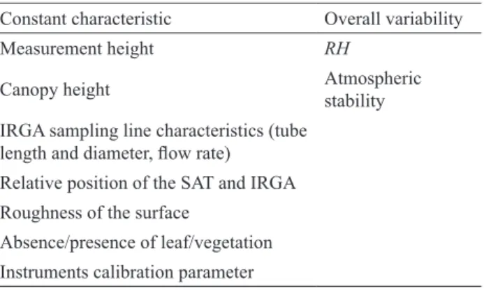
Step 1.1: Completeness of the averaging interval (AI) This step checks the number of originally missing re- cords in the time-series. The flagging system is based on the rules shown in Table 2: if the number of missing records is below 1% of what expected based on the acquisition frequency (i.e. 18000 for a 30-min long AI and sampling Table 1. List of the main characteristics that should be as
con-stant as possible, and of the variables to be represented, during the pre-processing phase. SAT = sonic anemometer thermometer, IRGA=infrared gas analyser, RH = relative humidity
Constant characteristics Overall variability
Measurement height RH
Canopy height Atmospheric stability IRGA sampling line characteristics (tube
length and diameter, flow rate) Relative position of the SAT and IRGA Roughness of the surface
Absence/presence of leaf/vegetation Instruments calibration parameter
Fig. 1. ICOS flagging system applied to the raw time series in the processing schemes to flag and to eliminate corrupted data. Left:
type of test, centre: criteria used in the flagging system, right: steps as numbered in the text and literature references, where it applies. N=number; SS=signal strength.
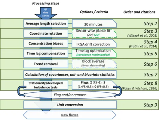
Fig. 2. ICOS scheme of the steps performed for the calculation of “raw” (not corrected) fluxes. Left: corrections applied, centre: options
selected or criteria used in the flagging scheme, right: steps as numbered in the text and literature references, where it applies. Green boxes indicate methods that require a pre-processing phase: green text between brackets indicates the method used in case the dataset is not available for the pre-processing. Dashed boxes indicate the steps used for the estimation of the uncertainty: text in black between brackets indicates the different method applied. FS= indicator for flux stationarity.
Fig. 3. Spectral corrections. Left: corrections performed, centre: options selected or criteria used in the flagging scheme, right: steps as numbered in the text and literature references, where it applies. ζ=stability parameter; Ts=sonic temperature; RH=relative humidity; CF=correction factor. Green boxes indicate methods that require a pre-processing on a long
frequency fs = 10 Hz) the flag is ‘0’. If this number is
between 1 and 3% flag is ‘1’, while if more than 3% of records are missing the flag is ‘2’.
Step 1.2: Absolute limits test
Unrealistic data values are detected by comparing the minimum and maximum values of all points in the record to fixed thresholds: values above and below the thresholds are considered unphysical. Thresholds defining plausibility ranges for the exclusion of records are defined as follow:
1. Horizontal wind (u and v): corresponding to the speci-
fication of the sonic anemometer (±30 m s-1 for Gill HS).
2. Vertical wind (w): ±10 m s-1.
3. Sonic temperature (Ts): -25°C to +50°C
(correspond-ing to the operation range of LI-7200).
4. Carbon dioxide (CO2) dry mole fraction (ΧCO2,d): 320 to 900 ppm.
5. Water vapour (H2O) dry mole fraction (ΧH2O,d): 0 to 140 ppt (corresponding to saturated water vapour pressure at max temperature, 12.3 kPa).
The records are discarded accordingly, and flags issued according to Table 2.
Step 1.3: De-spiking
Spikes are large, unrealistic deviations from the average signal, mainly due to electrical failures, instrument prob-lems, or data transmission issues, that need to be eliminated from the raw dataset to avoid biased (or fictitious) flux va- lues. At the same time, physical and large fluctuations of the measured variables must be retained. The method for spike determination, elimination and flagging is based on the median absolute deviation (MAD) as described in Mauder et al. (2013). MAD is calculated as:
(1) where: xi is the single record and <x> the median of the
data within a 30-min window. Records out of the following range are considered spikes:
(2) where: h is a parameter which is set to 7. The factor of 0.6745 allows the correspondence between MAD = 1 and one arithmetic standard deviation in case of Gaussian fre-quency distribution (Mauder et al., 2013). A flag is set according to Table 2, considering the number of discarded values (i.e. values identified as spikes).
Step 1.4: Wind direction test
Sonic anemometer arms and tower structures are known to distort the wind component. Also, other obstacles in the source area could create disturbances. According to this test, records are eliminated by default if the corresponding instantaneous wind direction lies within a range of ±10° with respect to the sonic arm, corresponding also to the direction of the tower. This range corresponds to the dis-torted wind sector in the calibration tunnel for the Gill HS due to the presence of the arm (Gill, personal communica-tion). Different ranges and additional sectors can however be defined according to site-specific characteristics, such as tower size and transparency. Flags are raised according to Table 1.
Step 1.5: Amplitude resolution test
The amplitute resolution test identifies data with a too low variance to be properly assessed by the instrument resolution. It is performed according to Vickers and Mahrt (1997). A series of discrete frequency distributions for half-overlapping windows containing 1000 data points each is built, moving one-half the window width at a time through the series. For each window position, data are grouped within 100 bins, the total range of variation covered by all bins is the smaller between the full range of occurring data and seven standard deviations. When the number of empty bins in the discrete frequency distribution exceeds a critical threshold value, the record is flagged as a resolution prob-lem. This test only produces a ‘0’ or ‘2’ flag. A flag = ‘2’ is raised if the number of empty bins in the discrete frequency distribution exceeds 70%.
Step 1.6: Drop out test
The drop out test is performed to flag sudden “jumps” in the timeseries which continue for a too long period to be identified by the despiking procedure (offsets). It is based on the same window and frequency distributions used for the amplitude resolution test. Consecutive points that fall into the same bin of the frequency distribution are tenta-tively identified as dropouts. When the total number of dropouts in the record exceeds a threshold value, the record is flagged for dropouts. This test only produces flag ‘0’ and ‘1’. The definition of the thresholds for this test varies depending on the location of the record in the distribution. For records between the 10th and the 90th percentile, if the number of consecutive points in the same bin in the discrete frequency distribution is higher than 10% of the total num-ber of records, the flag is ‘1’; for records beyond this range the threshold is set to 6% to consider the higher sensitivity to the extremes of the distribution.
Step 1.7: Instruments diagnostics
The Gill HS ultrasonic anemometer outputs information on possible failures in transducer communication, while the LICOR LI-7200 diagnostics include information on several Table 2. Flagging logic applied to steps from 1.1 to 1.4: 0 = good
quality; 1 = moderate quality; 2 = bad quality; N = number of records within the averaging interval (AI)
% missing/deleted records Flag
N<=1% 0
1%<N<=3% 1
possible failures of the instrument. If one of the diagnos-tics of the instrument detects a problem within the AI, no records are discarded, but the AI is flagged ‘2’. This is done based on the diagnostic codes produced by the sonic ane-mometer (issued at the selected frequency when an error occurs) and the IRGA (issued at 1 Hz). In addition, based on the average signal strength of the gas analyser, if this is above 90% in the AI a flag ‘0’ is produced; if between 75 and 90%, the flag is ‘1’; if below 75%, flag ‘2’ is produced. We stress that this value is not an absolute indicator of measurement offset, as the error induced by dirt in the cell depends on the spectral nature of the particles as well as on temperature. Furthermore, the user can reset the value to 100% after cleaning, setting the conditions of deployment at the cleaning as reference (LICOR, personal communica-tion). For that reason, the flag based on signal strength is indicative of the amount of dirt in the cell, and no data are discarded from its value.
Step 2: Selection of the length of the AI
The AI must be long enough to include eddies in the low frequency range of the spectrum, and short enough to avoid inclusion of non-turbulent motions and potential overesti-mation of turbulent fluxes. The widely accepted length of 30 min (Aubinet et al., 2000), associated with the spectral correction and the Ogive test described below, is deemed appropriate.
Step 3: Coordinate rotation of sonic anemometer wind data
One of the assumptions at the basis of the EC method is that, on average, no vertical motion is present (w = 0, where the overbar represent the mean value, i.e. the va- lue of w averaged over the AI). This means that the pole where the SAT is installed has to be perpendicular to the mean streamline. This assumption is not always met due to small divergences between the mean wind streamline and the ground, imperfect levelling of the instrument, or large scale movements, i.e. low frequency contributions (below 1/(length of AI) Hz). Hence, the coordinate frame has to be rotated so that the vertical turbulent flux divergence approximates the total flux divergence as close as possible (Finnigan et al., 2003). ICOS uses a modified version of the planar-fit (PF) method proposed by Wilczak et al., 2001 to rotate the coordinates of the sonic anemometer, often re- ferenced as sector-wise PF (Mammarella et al., 2007). This
PF method assumes that w = 0 only applies to longer
aver-aging periods, in the scale of weeks. Firstly, a plane is fitted for each wind sector to a long, un-rotated dataset including all the possible wind directions:
(3)
where w0, u0 and v0 are time series of mean un-rotated wind
components and b0, b1 and b2 are regression coefficients,
calculated using a bilinear regression. Then, for each aver-aging period the coordinate system is defined as having the vertical (z) axis perpendicular to the plane, the first horizon-tal axis (x) as the normal projection of the wind velocity to the plane, and the y-axis as normal to the other axes. The rotation matrix results to be time-independent, and it does not need to be fitted for each AI.
Also in this case a period of two months to be pre-processed is deemed sufficient to fit the plane with the number of sectors set to 8 by default. A different number of sectors might be considered on the basis of vegetation and topographic characteristics. For the detailed equations of the method see the above-mentioned publications, and also van Dijk et al. (2004). SAT orientation and canopy structure have a significant influence on the fit; this means that a new plane is fitted in case relevant changes occur to these parameters. In case the plane for a given wind sector is not well defined (e.g. not enough wind data from this direction), the closest valid sector is used to extrapolate the planar-fit parameter. If the time period for which data with a given site configuration is available is shorter than the required two months, a different method is applied (the 2D rotation method as in Aubinet et al. (2000) and a special flag is raised.
Alternative options: Different options suitable for the
coordinate rotation are available in the scientific literature, in particular the so-called 2D (Aubinet et al., 2000) and 3D (McMillen, 1988) rotations. The 3D rotation was excluded from the ICOS routine, while the 2D rotation is used for the estimation of the uncertainty. An overall discussion on alternative procedures is reported in the Results and Discussion section.
Step 4: Correction for concentration/mole fraction drift of the IRGA
The LI-7200 is subject to drift in measured mole frac-tions due to thermal expansion, aging of components, or dirt contamination. If an offset exists in the absorptance determination from the IRGA, not only the estimation of the mole fraction of the gas is biased, but also its fluctuations, due to the polynomial (non-linear) calibration curve used to convert absorptance into gas densities, with an impact on the calculation of turbulent fluxes (Fratini et al., 2014). Even if these issues are expected to be strongly reduced by the filter and heating in the tube and the periodic cleaning and calibrations, the problem might still arise. The method by Fratini et al., 2014 is used to correct the data: assuming that the zero offset in mole fraction readings (∆χg,w)
increas-es linearly between two consecutive field calibrations, the offset measured in occasion of calibration can be converted into the corresponding zero offset absorptance bias (∆a) through the inverse of the factory calibration polynomial, and spreading it linearly between two calibrations leads
each AI to be characterised by a specific absorptance off-set (∆ai). The inverse of the calibration curve is then used
to convert raw mole fraction values χg,w,i into the original
absorptances ai, and these latter corrected for ∆ai using:
(4)
ai,corr is then easily converted to mole fraction χg,w, corr,i
apply-ing the calibration curve, yieldapply-ing a corrected dataset which can be used for the calculation of fluxes. For the LI7200 the calibration function uses number densities: measure-ments of cell temperature and pressure are necessary for conversion to/from mixing ratios. After each calibration the method is applied to the data of the LI-7200.
Step 5: Time lag compensation
In EC systems, and particularly those using a closed path gas analyser, a lag exists between measurements of
w and gas scalars (sg), due to the path the air sample has to
travel from the inlet to the sampling cell of the IRGA, and due to the separation between the centre of the anemometer path and the inlet of the IRGA. In closed-path systems like the LI-7200, this time lag varies mostly with sampling vo- lume and flow in the tube, and depending on water vapour humidity conditions; more slightly with wind speed and direction. The different treatment of the electronic signal
might also contribute. Time series of w and sg need to be
shifted consequently to properly correct this lag, or the covariances will be dampened and the fluxes underestimat-ed. Even if a “nominal” time lag can be easily calculated based on the volume of the tube and the flow rate of the pump, this lag can vary with time due to different rea-sons such as accumulation of dirt in the filter of the tube, slight fluctuations of the flow rates, and relative humid-ity (RH) content. It may also be different between gases,
as molecules of H2O tend to adhere more to the walls of
the tube than other gases like CO2, resulting in a higher
time lag (Ibrom et al., 2007b; Massman and Ibrom, 2008; Mammarella et al., 2009; Nordbo et al., 2014). The method used to correct this lag in ICOS is called “time lag optimi-sation”, as it consists in a modification of the well-known covariance maximisation approach (Aubinet et al., 2012). Both methods seek an extremum in the cross correlation
function between w and the sg that has the same direction
as the flux (e.g. a minimum for a negative flux). However, in the time lag optimisation the sizes of the window where to look for the time lag are computed continuously instead
of being constant. For H2O, different windows and nominal
lags are automatically computed for different RH classes in order to take into account the dependence of the time lag on
RH. The width and centre of the windows are statistically
computed on the basis of an existing, long enough dataset, subjected to the cross correlation analysis: the nominal time
lag (TLnom) is calculated as the median of the single time
lags (TLi), and the limits of the window (TLrange) are defined
by:
(5) where: <> indicates the median operator. For water vapour, this procedure is replicated for each RH class, and a diffe- rent TLrange is calculated for any different RH. TLnom is used
as default value to be used as time lag in case the actual time lag cannot be determined in the plausibility window (i.e. if an extremum is not found). This method requests the execution of Steps 1-5 of the standard processing chain on a sufficiently long dataset to calculate the time lag parameters. The dataset has to cover a range of climatic conditions as broad as possible, and its minimum length is two months. The two time series are then shifted accord-ingly with the calculated time lag in every AI. In the case of a shorter period with a given site configuration, the method is switched to the “traditional” covariance maximisation (i.e. using a fixed window). A special flag indicates the occurrence of this different method applied to the final users.
Alternative options: The most widespread alternative
method consists in maximising the covariance in fixed
windows, a less flexible approach especially for H2O
con-centrations at different values of RH. See also the Results and discussion section.
Step 6: Calculation of background signal and fluctuations The procedure of separating background signals (x) and fluctuations (x’) of a time series x = x(t) is based on Reynolds averaging (Lee et al., 2004):
x’=x – x. (6)
This operation introduces a spectral loss, especially at the low frequency end of the spectra (Kaimal and Finnigan, 1994, see Step 10.2). The method used in the main process-ing chain of ICOS is the so-called block averagprocess-ing (BA). The effect on the spectra can be conveniently represent-ed with a high-pass filter, and then correctrepresent-ed (see below). Block averaging consists of time averaging all the instan-taneous values in an AI, and the subsequent calculation of fluctuations as instantaneous deviations from this average (xBA):
(7) (8) where: N is the number of digital sampling instants j of the time series x(t) (discrete form) in the AI. As the mean is constant in the averaging interval, BA fulfils Reynolds averaging rules (Lee et al., 2004) and impacts at a lower degree the spectra (Rannik and Vesala, 1999).
Alternative options: two alternative methods are widely
used in the EC community, namely the linear de-trending (LD, Gash and Culf, 1996) and the autoregressive filtering (AF, Moore, 1986; McMillen, 1988). The LD is used as an alternative method to calculate the uncertainty in the data. An overall discussion is reported in the respective section.
Step 7: Calculation of final covariances and other statistics
After the steps described in the above, the final covarian- ces are calculated, together with other moment statistics. In turbulent flows, a given variable x can be statistically described by its probability density function (PDF) or associated statistical moments. Assuming stationarity and ergodicity of x (Kaimal and Finnigan, 1994) we are able to calculate statistical moments, characterizing the PDF of x, from the measured high frequency time series x(t).
Single-variable statistics include moments used for flag-ging data: mean value (first order moment), variance (and thus standard deviation), skewness and kurtosis, i.e. se- cond, third and fourth order moments. Indicating with n the moment, we can resume all of them in a unique equation:
(9) where: x'n indicates the n-th moment, N = l
AI fs, lAI the length
of the averaging interval (s) and fs the sampling frequency
(Hz), xj the instantaneous value of the variable x, x the mean
value.
In the same way, moments of any order associated with joint probability density function of two random variables can be calculated. In particular, covariances among verti-cal wind component w and all other variables also need to be calculated. In general, the covariance of any wind com-ponent uk or scalar sg with another wind component ui is
calculated as follows:
(10) (11) where: uk, with k =1, 2, 3, represents wind components ui, vi
or wi, and the subscript j indicates the instantaneous values of the corresponding scalar or wind component from 1 to N.
Please note that this step refers to the calculation of the final covariances used for the calculation of the fluxes. However, statistics are also calculated after each step of the processing.
Step 8: Quality control on covariances: steady-state and well developed turbulence tests
These two tests (Foken and Wichura, 1996), applied to the calculated covariances, are necessary to check the verification of basic assumptions of the EC method, i.e. the
stationarity of the variables in the AI and the occurrence of conditions where the Monin-Obukhov similarity theory applies.
Step 8.1 Steady-state test (Foken and Wichura, 1996) Typical non-stationarity is driven by the change of meteorological variables with the time of the day, changes of weather patterns, significant mesoscale variability, or changes of the measuring point relative to the measuring events such as the phase of a gravity wave. The method to define non-steady-state conditions within AI by Foken and Wichura (1996) uses an indicator for flux stationarity FS:
(12) where: m = 6 is a divisor of the AI defining a 5 mins win-dow. x's'(AI/m) is the mean of the covariance between w and s
calculated in the m windows of 5 min:
(13) The flux is considered non-stationary if FS exceeds 30%.
Step 8.2 Well-developed turbulence test (Foken and Wichura, 1996)
Flux-variance similarity is used to test the development of turbulent conditions, where the normalized standard deviation of wind components and a scalar are parame- terized as a function of stability (Stull, 1988; Kaimal and Finnigan, 1994). The measured and the modelled norma- lized standard deviations are compared according to:
(14) where: variable x may be either a wind velocity component
or a scalar, and x* the appropriate scaling parameter. The
test can in theory be done for the integral turbulence char-acteristics (ITC) of both variables used to determine the covariance, but it is applied only on w (more robust), with the exception of w’u’ for which both parameters are calcu-lated, and the ITCσ is then derived using the parameter that
leads to the higher difference between the modelled and the measured value (numerator Eq. (14)). The models used for (σx/x*)mod are the ones published in Thomas and Foken
(2002) (Table 2). An ITCσ exceeding 30% is deemed as the
absence of well-developed turbulence conditions. Step 9: From covariances to fluxes: conversion to physical units
Calculated covariances as described above need to be converted in physical units, mainly via multiplication by meteorological parameters and constants. The subscript ‘0’ indicates that the fluxes are still not corrected for spectral attenuation, and the sonic temperature not yet corrected for the humidity effect:
(15) Flux of CO2 (μmol m-2 s-1): (16) Flux of H2O (mmol m-2 s-1): (17) Flux of evapotranspiration (kg m-2 s-1) (18) Flux of latent heat (W m-2)
(19) Flux of momentum (kg m-1 s-2)
(20) Friction velocity (m s-1)
(21) where χCO2,d is the mixing ratio of CO2, χv,d that of water
vapour; Mv the molecular weight of water vapour: 0.01802
kg mol-1; λ the specific evaporation heat: (3147.5-2.37Ta)
103; and pd = p
a – e is the dry air partial pressure. Gas fluxes are calculated using the dry mole fraction data, which are not affected by density fluctuations, differently from e.g. mole fraction (Kowalski and Serrano Ortiz, 2007). As the ICOS selected IRGA is able to output the gas quantities in terms of dry mole fraction, this is a mandatory variable to be acquired at ICOS stations. The IRGA applies a transfor-mation in its software to convert mole fraction in dry mole fraction using the high-frequency water vapour concentra-tion data.
Steps to calculate the air density ρa,m:
a) (air molar volume); (22)
b) (water vapour mass concentrations); (23)
c) (dry air mass concentrations); (24)
d) (25)
Steps to calculate the air heat capacity at constant pres-sure cp:
a)
(water vapour heat capacity at constant pressure);
(26) b)
(dry air heat capacity at constant pressure); (27)
c) (specific humidity); (28)
d) (29)
Step 10: Spectral correction
In the frequency domain, the EC system acts like a fil-ter in both high and low frequency ranges. Main cause of losses at the low frequency range is the finite AI that limits the contribution of large eddies, together with the method used to calculate turbulent fluctuations (see Step 6), which acts as a high-pass filter. Main cause for losses at the high frequency range is the air transport system of the IRGA, together with the sensor separation and inadequate fre-quency response of instruments leading to the incapability of the measurement system to detect small-scale varia-tions. To correct for these losses, the correction is based on the knowledge of the actual spectral characteristics of the measured variables, and on the calculation of the difference with a theoretical, un-attenuated spectrum. A loop is pre-sent in this part of the processing chain (Fig. 3), where the corrections are performed iteratively to refine the calcula-tion of the spectral parameters.
Step 10.1: Calculation and quality of spectra and cospectra
Calculation of power spectra (and cospectra) is a fun-damental step to perform spectral analysis and correction of the fluxes. Calculated fluxes are composed of eddies of different lengths, i.e. signals of different contributions in the frequency domain: the knowledge of the spectral cha- racteristics of the EC system and the shape of the model spectra is crucial for the execution of spectral corrections. In ICOS processing the calculation of power (co)spectra, at the basis of the analysis in the frequency domain, is per-formed using the Fourier transform (Kaimal and Finnigan, 1994), which allows to correct the spectral losses analys-ing the amount of variance associated with each specific frequency range. Validity of the Fourier transform for EC measurements is supported by the Taylor’s hypothesis of frozen turbulence (Taylor, 1938). For further details on the theory (Stull, 1988).
Full spectra and cospectra are calculated for each AI over a frequency range up to half the acquisition frequency (Nyquist frequency). The algorithm used to calculate the Fourier transform is the FFT (Fast Fourier Transform), which is applied to the time series after their reduction and tapering (Kaimal and Kristensen, 1991). In order to apply the FFT algorithm, the number of samples used will be equal to the power-of-two closest to the available
number of records (i.e. 214 for 10 Hz and 215 for 20 Hz
data). Binned cospectra are also calculated to reduce the noise dividing the frequency range in exponentially spaced frequency bins, and averaging individual cospectra values that fall within each bin (Smith, 1997). Finally, spectra and cospectra are normalised using relevant run variances and covariances, recalculated for the records used for (co)spec-tra calculation, and averaged into the exponentially spaced frequency base. The integral of the spectral density rep-resents the corresponding variance and the integral of the cospectral density the corresponding covariance (Aubinet
et al., 2000). Normalisation by the measured (co)variances
forces the area below the measured (co)spectra to 1, but the ratio between the areas (model/measured (co)spectra) is preserved. Thus, addressing losses in the different ranges of frequency allows having a flux corrected for spectral losses due to different causes.
The approach to compensate for spectral losses is dif-ferent in the low and high frequency ranges, and for fluxes measured by the SAT and gas scalars. All the methods used in ICOS processing are based on Fourier transforms, and rely on the calculation of an ideal (co)spectrum unaffect-ed by attenuations (CSId,F), on the definition of a transfer
function (TF) characteristic of the filtering made by the measuring system (both functions of frequency f (Hz)), and on the estimation of a spectral correction factor (CF):
(30) Multiplying the attenuated flux for CF leads to the spec-tral corrected flux. Several parameterisations exist of the ideal cospectrum, which depends mainly upon atmospheric stability conditions, frequency, horizontal wind speed, measurement height and scalar of interest. One of the most used model cospectrum is based on the formulation by Kaimal et al. (1972), and is implemented also in the ICOS processing when an analytic approach is adopted. In the following we describe the application of spectral correc-tions separately for the different frequency ranges and the different types of flux.
Step 10.2: Low-frequency range spectral correction (Moncrieff et al., 2004)
Losses at the low end of the (co)spectra mainly arise when the necessarily finite average time is not long enough to capture the full contribution of the large eddies to the fluxes. The methods used to separate fluctuations from the background signal enhance this event, excluding eddies with periods higher than the averaging interval. This cor-rection is based on an analytic approach.
In this case the ideal cospectrum is based on the formu-lation of Moncrieff et al. (1997), while TF represents the dampening at the low frequency range. Application of TF to the cospectra gives the attenuation due to frequency losses, and because of the proportional relationship between a flux
and the integral of its cospectrum, a spectral correction fac-tor can be easily calculated. This can be done on the basis of the method used to separate the fluctuations from the rest, which acts as a filter as said above. From Rannik and Vesala (1999) and Moncrieff et al. (2004) we get the high-pass transfer function corresponding to the block average:
(31) where: lAI is the length of AI (s). The corresponding
correc-tion factor (HPSCF) is calculated as the ratio:
(32) where: fmax is the higher frequency contributing to the flux,
and CSId,F (f) represents the model describing the normalised
un-attenuated cospectrum for a given flux F, depending on the natural frequency f.
Step 10.3: High-frequency range spectral correction Corrections of the high frequency part of the spectra and cospectra are more detailed as this end of the spectra is defined and several publications exist to correct the cor-responding attenuations.
A fully analytic method is applied to correct H and τ, an experimental method for the other fluxes.
Step 10.3.1: Fully analytic method (Moncrieff et al., 1997)
This method is used in ICOS processing only to cor-rect anemometric fluxes (i.e. H and τ). With this method both the ideal cospectral densities CSId,F and the low-pass
transfer function LPTFSAT are calculated in an analytical
(theoretical) way. LPTFSAT results from a combination of
transfer functions each characterising a source of attenu-ation, as described among others in Moore et al. (1986); Moncrieff et al. (1997), from where all of the transfer func-tions reported below are taken, while the cospectral model is based on Kaimal et al. (1972):
1. LPTFSAT of sensor-specific high frequency loss:
(33) where: τs the instrument-specific time constant.
2. TF of the sonic anemometer path averaging for w and for Ts, respectively:
(34) (35) where fw is the normalised frequency:
(36) and lp is the path length of the sonic anemometer transducers.
The final transfer function of the analytic method results from the product:
(37)
Application of Eq. (36) using LPTFSAT allows the
cal-culation of the corresponding low-pass spectral correction factor for sonic fluxes (LPSCFSAT).
Step 10.3.2: Experimental method (Ibrom et al., 2007a; Fratini et al., 2012)
The experimental method firstly described in Ibrom et
al. (2007a) and then refined in Fratini et al., 2012 is applied
to gas scalars. Assuming spectral similarity, this method derives in-situ the un-attenuated spectral density, assuming that the spectrum of the sonic temperature is unaffected by the main sources of dampening, and then represents a proxy for the ideal spectrum of gas concentrations.
The effect of the measuring system is approximated with a first-order recursive, infinite impulse response fil-ter (IIR), whose amplitude in the frequency domain is well approximated by the Lorentzian:
(38)
where: Smeas represents the ensemble averaged measured
spectra, and STs the ensemble averaged spectra of sonic
temperature representing the ideal unaffected spectrum.
This way, the cut-off frequency fc can be determined
in-situ based on the actual conditions of the measuring system
and of the ecosystem using Eq. (38). For water vapour in closed-path systems, this fit is performed for different classes of RH, and then the general cut-off frequency is extrapolated fitting the single cut-off frequencies fci to an
exponential function:
(39) where: a, b and c are fitting parameters.
The low-pass spectral correction factor for gas scalars is then calculated as:
(40)
where: A1 and A2 are parameters determined by filtering
sonic temperature time series with the low pass recursive filter using varying values of the filter constant, in both sta-ble and unstasta-ble atmospheric stratifications (see Ibrom et
al., 2007a for details). This leads to a LPSCFGAS that not
only depends on stratification, but is also site-specific. Both the gas (attenuated) and the sonic temperature (un-attenuated) spectra are intended as ensemble-averaged spectra. Averaging is performed on binned spectra (see Step. 10.1) selected for high-quality. This quality control is based on the same tests applied to the time series (see above), including also skewness and kurtosis. Moreover, only spectra for AIs with high fluxes are used for the deter-mination of high-quality spectra, thus excluding periods of low turbulence and low signal-to-noise ratio. Thresholds are therefore applied on the calculated fluxes before spec-tral correction. Thresholds are defined differently between stable and unstable atmospheric conditions: in the latter case thresholds are less strict, in order to reduce the risk of missing night-time spectra. The situations excluded are reported in Table 3. In addition, H2O spectra are sorted into
nine relative humidity classes.
Fratini et al. (2012) suggested a modification of this method to provide a refinement in case of large fluxes. The
calculation of LPSCFGAS is as above (Eq. (40), but see the
original papers for a difference in the approach) only for small fluxes, while for large fluxes it becomes:
(41) thus applying the general Eq. (38) with measured data, using the lower frequency allowed by the averaging inter-val (fmin) and the Nyquist frequency (fmax=fs/2); using the
current cospectral density of sensible heat (CSH) as a proxy
for the ideal, unaffected cospectral density for each AI; and
using the TF determined by the low-pass filter with the fc
determined in-situ, dependent from RH in the case of H2O
fluxes.
“Small” fluxes are defined on the basis of the following thresholds: |H| and |LE| < 20 W m-2; |F
CO2|< 2 μmol m2 s-1.
The dataset used to calculate the spectral characteristics
and to extrapolate LPSCFGAS should be representative of
the overall variability of micrometeorological conditions, especially RH and the overall ecosystem characteristics (dynamics of canopy development) and EC system (not Table 3. Thresholds used to discard spectra from the calculation of ensemble averages in spectral corrections, depending on
atmos-pheric stability. Stability conditions are defined by the Obhukov length L
Flux Unstable conditions (-650 < L < 0) Stable conditions (0 < L < 1000)
|H0| < 20 W m-2; > 1000 W m-2 < 5 W m-2; > 1000 W m-2
|LE0| < 20 W m-2; > 1000 W m-2 < 3 W m-2; > 1000 W m-2
|FCO2,0| < 2 μmol m-2 s-1; > 100 μmol m-2 s-1 < 0.5 μmol m-2 s-1; > 100 μmol m-2 s-1
changing setup). In Table 1 the most important characteri- stics that have to be homogeneous throughout the overall period of spectral characterisation are reported, together with the most important conditions whose variability has to be represented as much as possible. This means that even if in theory the full-year period used in ICOS pro-cessing is sufficiently long, every time the setup is changed a new characterisation of (co)spectra is needed. For fast-growing species an exception is needed, due to both the fast changes in canopy height, and the consequent adaptation of the measurement height made at the stations to keep the distance between measurement and displacement height as constant as possible. In this case a two-week period is deemed enough to calculate spectral parameters, and the station team should ensure as much as possible periods of minimum two weeks with a constant measurement height and the same EC configuration in general. In any different case when a given configuration is operational for less than two weeks, the fully analytic method for spectral correc-tions is applied (Moncrieff et al., 1997), more generic but with no need of calculating spectral parameters on a long dataset. A special flag is issued accordingly.
Alternative options: several alternatives are published
in the scientific literature for the high-frequency correction for gas scalars, belonging to the two big groups of analytic and experimental methods. In the Results and discussion section is presented a wider discussion on alternative options.
Step 10.4: Losses due to instrumental separation (Horst and Lenschow, 2009)
The spatial separation between the gas analyser (inlet) and the sonic anemometer path causes attenuation in the high-frequency range of the cospectra which can be often neglected. However, it may become important especially over smooth surfaces at low measurement heights, due to the dependence of the cospectral peak frequency (fp) on the
atmospheric stratification (fp shifts to lower frequencies
with increasing (z-d)/L, Kaimal and Finnigan, 1994). To account for these losses a correction method was developed by Horst and Lenschow (2009), which depicts the flux of a scalar measured at a distance ls from the centre of the
son-ic path as a function of the distance itself and the frequency at the peak of the corresponding cospectrum according to:
(42) where: F0 is the un-attenuated flux, np = fp (z-d)/u, fp being
the frequency at the peak of the cospectrum and z the meas-urement height. This formulation can then be modulated for the three linear components of the 3D distance respective to the wind direction, i.e. along-wind, cross-wind and vertical. However, the along-wind component is mostly corrected when compensating for the time lag. For that reason, the method implemented in ICOS only uses the cross-wind and the vertical component of this correction.
Step 10.5: Calculation of the spectral correction factor The implementation of the above-described methods is based on the calculation of different transfer functions in the frequency domain representing the dampening at both low and high frequencies, characterised by a specific cut-off frequency. Application of transfer functions to the cospectra gives the attenuation due to frequency losses. A correction factor including all the spectral corrections as a whole can be calculated. In practical terms, this is done by
multiply-ing HPTFBA and LPTFSA, resulting in a band pass transfer
function for sonic variables correction (BPTFSA) which is
then inserted in Eq. (30) to derive a unique spectral cor-rection factor. For the gas variables, whose high-frequency attenuation was instead calculated with the experimental approach, the HPSCF is first used to correct the gas fluxes for the high-pass filtering effects and then the LPSCF is applied for the low-pass filtering effects.
Step 11: Humidity effect on sonic temperature
Sonic temperature (Ts) is used to calculate the covarian-
ce w'Ts', which approximates the buoyancy flux, as Ts is
close to virtual temperature (Tv). The sensible heat flux
(H) is defined as the covariance of w with the real air
tem-perature, which may deviate from Ts for 1-2% due to the
dependency of sound velocity on water vapour pressure (Aubinet et al., 2012):
(43) where: T is the real absolute temperature, e the partial pres-sure of water vapour and p the air prespres-sure. A correction for this effect is thus needed, and is based on papers by Schotanus et al. (1983) and van Dijk et al. (2004), using the following equation:
(44) where: Hcorr represents the sensible heat flux corrected for
humidity effect, Hsp approximates the buoyancy flux
cor-rected for spectral losses, ρa,mcp is the product of air density
and air heat capacity, Esp is the evapotranspiration flux
cor-rected for spectral losses, and q the specific humidity. Step 12: Iteration and calculation of atmospheric stability Some of the above mentioned methods depend on atmospheric stability. This characteristic is commonly described using the parameter ζ, defined as:
ξ (45)
where: d is the displacement height, i.e. the height at which the wind speed would assume zero if the logarithmic wind profile was maintained in absence of vegetation. It is mostly calculated from canopy height (hc) as d = 0.67hC. However,
in case the ICOS station has a wind profile (not manda-tory), this parameter can be calculated more accurately. L is instead the Obukhov length:
(46) where: Tp is the potential temperature (K), calculated from
air temperature as (p0 is the reference
pres-sure set to 105 Pa), κ = 0.41 is the von Kármán constant
and g is the acceleration due to earth’s gravity (9.81 m s-2).
Fluxes are thus involved in the calculation of L, meaning that some of the spectral correction methods above lead to a modification of L itself, and hence of ζ, which is used in spectral correction, thus there is the need for iteration to achieve higher precision (Fig. 3, Clement, 2004).
Step 13: Quality-control tests on calculated fluxes After the calculation of the fluxes as described above, tests can be performed for a further exclusion of bad quality data, which are based on the spectral analysis.
Step 13.1: Spectral correction factor test
Spectral correction at both low and high frequency ranges basically estimates the attenuations of the EC sig-nal due to different causes, and corrects for this losses. If however the losses turn out to be very big, i.e. if the EC system is capable of detecting only a small portion of the spectrum, the AI is discarded. The method for filtering data after fluxes calculation takes into consideration the portion of the power spectrum measured by the EC system: if the spectral correction factor obtained applying the spectral correction method is below 2, i.e. if more than half of the power spectrum has been detected by the EC system, the flag is ‘0’. If the spectral correction factor is between 2 and 4, i.e. if the EC system is capable of detecting less than half but more than one third of the power spectrum, the flag is ‘1’. Otherwise (less than one third of the power spectrum detected), flag is ‘2’ and the calculated flux eliminated.
Step 13.2: Ogives test
The finite ogive (Og) is defined as the cumulative co-spectrum. At each given frequency, the ogive represents the integration of the co-spectrum from the current frequency to the Nyquist frequency. Then its value at the lowest fre-quency provides the integration of the full co-spectrum, which corresponds to the covariance (Berger et al., 2001). Ogives can be used to evaluate the suitability of the chosen
AI. Provided that conditions of stability are met in the AI,
the typical form of an Ogive for EC fluxes has an S-shape: significant deviations from this shape indicate problems in the measured covariance. In particular, if the ogive has a large slope at the lowest frequencies, it means that signifi-cant fractions of the flux occur at these timescales, and then that the chosen AI may not be long enough. To use Ogives as a test, a smoothing filter is applied to reduce scatter at the
higher frequencies, and the Ogives are normalised to the corresponding covariances to make them comparable. To determine the slope in the low frequency range, two thresh-olds are selected as in Spirig et al. (2005): the frequency threshold (0.002 Hz) determining the lower part of the frequency range, and the threshold (15%) for the value of the normalised Ogive at this given frequency, above which the corresponding AI is considered too short and a flag ‘1’ raised. However, this flag is not used for the calculation of the overall data quality.
Step 14: Calculation of overall data quality flags
First the indicators of the quality-control tests applied to the covariances in Step 8 are combined in a single flag using the flagging system based on Mauder and Foken (2006). A system of nine flags is developed for both tests
cor-responding to as many ranges of FS and ITCσ, and then
combined in a 0-1-2 flag system: if both tests yield a value lower than 30% the flag is ‘0’, if at least one of them is between 30% and 100% the flag is ‘1’, and if at least one is above 100% the flag is ‘2’. All the flags produced as described in this manuscript are combined to decide wheth-er or not the flux value for an AI will be discarded. If at least one of the flags is ‘2’, the corresponding flux value is discarded. If four or more of the other tests have a flag ‘1’ the AI is discarded as well. In Table 4 we report a summary of all the tests performed and used in the overall QC. From that list we intentionally excluded the following indicators, which are not part of the overall data quality control:
1. signal strength information from IRGA;
2. flag indicating periods with methods for spectral cor- rection, coordinate rotation and time-lag compensation dif- ferent from the standard ones (lack of data for the pre- processing);
3. Ogives test. Post-processing stages
In the following a synthetic description of the ICOS treatment applied to the processed raw-data is presented. This section is organised in sub-sections called Stages to avoid confusion with the Steps above. It starts from the description of the assessment of data uncertainty, includes Table 4. Tests used in the overall quality estimation
TEST DATA FLAGS
Completeness of the AI raw 0, 1, 2
Absolute limits raw 0, 1, 2
Spike detection raw 0, 1, 2
Wind direction raw 0, 1, 2
Amplitude resolution raw 0, 2
Drop-out raw 0, 1
Instruments diagnostics raw 0, 2 Steady-state + ITC covariances 0, 1, 2 Spectral correction factor fluxes 0, 1, 2
the organisation of the Near Real Time (NRT) processing applied daily to the raw data, and finally lists the actions needed to filter out low quality periods or suspicious data points, to account for non-turbulent fluxes and to fill the gaps created by filtering and missing data. The footprint analysis is introduced. The description of the post-process-ing in this section is general, but it has the aim of clarifypost-process-ing that after the turbulent flux calculation a number of addi-tional and crucial steps are needed in order to calculate the final NEE estimate.
Stage 1: Uncertainty estimation
Due to the complexity of the method, the overall uncer-tainty of the EC technique derives from a diverse pattern of sources of errors (Richardson et al., 2012): from the instru-ment-related measuring errors to the non-occurrence of the conditions at the basis of the method, from the random error due to one-point sampling to the uncertainty introduced by the processing chain itself. Also the filtering of periods with too low turbulence (Stage 5) is responsible for a fraction of uncertainty. The estimation of uncertainty is under dis-cussion in the EC community (Vickers and Mahrt, 1997; Finkelstein and Sims, 2001; Hollinger and Richardson, 2005; Dragoni et al., 2007; Mauder et al., 2013). Here we describe the estimation of random uncertainty and that introduced by the choice of the data processing scheme. Finally we mention how the different approaches used in
the post-processing (namely the u* thresholds calculation
and the partitioning methods) depict the overall variability of the final fluxes.
Stage 1.1: Flux random uncertainty
The flux random uncertainty due to the limitations of sampling, also known as turbulence sampling error (TSE), is estimated following the approach by Finkelstein and Sims (2001). The Integral Turbulence time-Scale (ITS) is derived from the integral of the auto-covariance function of the time-series φ = w' s' normalised by the variance of φ (Rannik et al., 2016), where φ contains the instantaneous covariance values between w and s measured over AI. Then
the random uncertainty (εF,rand) is estimated, based on the
calculation of the variance of covariance:
(47) where: N is the number of raw measurements in the AI, represents a number of samples large enough to capture the
integral timescale, calculated as ITS*fs, and and
are auto-covariance and cross-covariance terms for atmos-pheric fluxes, which can be estimated for lag h as:
(48) (49) In the ICOS processing h is set to 200 s, as recommended by Rannik et al. (2016).
Stage 1.2: Uncertainty in the half-hourly turbulent fluxes due to the processing scheme
The processing options used to calculate the fluxes contribute to the overall uncertainty. At present there is no a widely agreed strategy conceived to calculate this uncer-tainty in the scientific community, but few studies exist (Kroon et al., 2010; Nordbo et al., 2012; Richardson et al., 2012; Mauder et al., 2013; Mammarella et al., 2016).
The main processing scheme proposed currently for ICOS ecosystems and described in the present manuscript aims at a maximum degree of standardisation. However, as shown above, other processing options might also be valid and reliable. This leads to an uncertainty due to the process-ing scheme. For evaluatprocess-ing this portion of the uncertainty, some alternative processing methods are proposed in a fac- torial approach together with the methods used in the main processing chain, which are assumed to contribute the most to the variability in the flux estimation, and which are equally reliable for the ICOS setup: the 2D coordinate rota-tion and the linear de-trending (LD) approach. Hence, the processing scheme described is replicated four times, cor-responding to the factorial combination of the suggested options (BA/LD combined with 2D/PF). This scheme does not apply in the pre-processing, neither in the NRT process-ing scheme (Stage 2).
For each flux of each AI, the factorial combination re- sults in four quantities of calculated fluxes. Since there are not tools to establish a priori which is the combination of processing options providing unbiased flux estimates, we assume that the “true unobserved” flux quantity is equally likely to fall anywhere between the upper and lower limit derived from the 4 processing schemes. This translates in assuming that the PDF of flux estimated by a multiple processing scheme is better approximated by a continuous uniform distribution (BIPM et al., 2008). Hence, the mean value is calculates as:
(50) and the uncertainty is quantified as:
(51)
Fs denotes the flux of a generic scalar s, while max (Fs,j)
and min (Fs,j) are the maximum and minimum flux values
respectively among those calculated in j=1,…,4 processing schemes.
εF,proc represents the between-flux variability due to diffe-
rent processing schemes. However, different processing schemes lead also to different values of εF,TSE, whose varia-
bility needs to be taken into account for a proper quantifi-cation of the random uncertainty affecting half-hourly flux time series. To this aim, the TSE associated with the half-hourly Fs,mean is estimated by averaging the four values of εF,TSE,j estimated for each processing scheme:
(52) Stage 1.3: Combination and expanded random uncertainty
The combined random uncertainty εF,comb is then obtained
by combining εF,TSE and εF,proc via summation in quadrature:
(53) The expanded uncertainty (see also BIPM et al., 2008) is achieved by multiplying the combined random uncer-tainty with a coverage factor of 1.96 in order to define the 95% confidence interval of the true unobserved flux esti-mates as follows:
(54) The magnitude of the confidence interval is then pro-portional to the importance of the processing scheme in the flux estimates uncertainty.
Stage 2: Near-real time (NRT) data processing
Near-real time (NRT) data processing is an important tool for ICOS, as it allows updating fluxes on a daily basis for real time visualisation of the fluxes and possible inges-tion in modelling activities. It also enables ETC to send warnings to principal investigators (PIs) in case of errors or failures of the system. A prompt reaction is demanded to the PI so that problems at the station can be solved swiftly, and the high-quality standard of data maintained. The NRT processing is applied on a moving window of 10 days. In order to achieve a high quality standard, the same processing chain as for the final data (main process-ing) is applied as far as possible. However, certain options are not applicable to NRT processing, as detailed below. This translates in applying Steps 1 – 14 of the main pro-cessing, with the exclusion of Step 4 and some differences in Steps 3, 5, 10 (Figs 2-3). Step 4 corresponds to the cor-rection of concentration/mole fraction drift of the IRGA, which is not included in the NRT processing scheme, as it uses data from calibrations that may only become available afterwards. Differences in Steps 3, 5 and 10 occur due to the need for a pre-processing to calculate parameters used in these corrections. The corresponding parameters are cal-culated once on a given dataset of two months, and then used in the daily runs for flux calculation. It is therefore important to keep the distance between the measurement height and the displacement height as constant as possible, by dynamically move the system according to the height increment in stations with fast-growing vegetation.
A different method is used when the two-month dataset is not available. This applies, in addition to the beginning of the measurement period, every time a re-
levant change occurs in the instrument setup, or the eco-system characteristics become different from those used in the pre-processing. This translates in a temporary (possibly less accurate) flux computation.
NRT processing stops after the calculation of net eco-system exchange (NEE) by summing up the storage term to FCO2, excluding gap-filling and filtering based on friction
velocity (u*) methods (see below). Also, the uncertainty
estimation is limited to the random component, i.e. the fac-torial combination of options is not applied to estimate the uncertainty due to the selection of processing methods.
Step 1 and Step 2 are the same as in the main process-ing. The rotation of the coordinate system of the sonic is also the same (sector-wise planar fit, Step 3) only if the corresponding parameters, calculated on a period of at least two months, are available: these coefficients are then used for the daily processing, as long as no relevant changes occur, or as long as their calculation will be updated. When the two-month dataset is not available, the 2D rotation is applied until a new two-month dataset will be complete.
As stated above, Step 4 is not applied in the NRT. Step 5,
i.e. the time lag optimisation to align the data streams of the
sonic and the IRGA, is applied with the same limitations of Step 3: a two-month dataset is used once for the calculation of the statistic parameters of the method, which are then used for the daily processing. When relevant changes hap-pen in the setup of the EC system the parameters need to be updated. In this case, and whenever a coherent two-month dataset is not available, the classic approach of covariance maximisation is applied. Step 6, Step 7, Step 8, and Step 9 are executed following the same methods as in the main processing. Step 10 is partly different in case a long enough dataset of two months is not available to estimate the low-pass filter characteristics and the spectral model parameters of the experimental high-frequency spectral corrections (Step 10.3.2). Even if in theory the size of the data window depends on the characteristics listed in Table 1, for stand-ardisation a period of minimum two months is required. As in the main processing scheme, for fast-growing species a two-week period is deemed enough to calculate spectral parameters, and the PI has to avoid a more frequent change of the EC system configuration. When the dataset is not available, the fully analytic method (Moncrieff et al., 1997) is temporarily applied, and the Step 10.4 is not needed. In any case, the sub-Steps 10.1, 10.2 and 10.3.1 are the same of the main processing scheme. Step 11, Step 12, Step 13 and Step 14 in the NRT processing scheme are identical to the main processing scheme.
Stage 3: Storage component
The NEE is calculated from the turbulent flux of CO2
by summing it up with the fluxes arising from the change in storage below the eddy covariance instrumentation (Nicolini et al., 2018). The storage change term is