Prediction of risk of an event using sensor signals, with application to the prevention of driving accidents due to drowsiness

(1)

Prediction of risk of an event

using sensor signals,

with application to the prevention of

driving accidents due to drowsiness

Author: Pouyan Ebrahimbabaie

Supervisor: Professor Jacques G. Verly

A thesis submitted in partial fulfillment of the requirements for

the degree of Doctor of Philosophy in Engineering Sciences

November 2020

Department of Electrical Engineering and Computer Science Faculty of Applied Sciences

(2)

(3)

The drowsy state is an intermediate state between alert wakefulness and sleep. Drowsiness is a major cause of accidents in many areas of human activity, and transportation is probably the single most important source of drowsiness-related accidents. It is thus paramount to continuously, and in real-time, monitor the level of drowsiness (LoD) of a driver, and to devise in-car safety systems to help prevent related accidents.

For road vehicles, it is useful to distinguish between three categories of drowsi-ness monitoring in-vehicle systems, respectively monitoring the car behavior, the driver behavior, and the driver physiology. The systems in the last category are the only ones that can truly measure the state of drowsiness of a person. These systems are the only ones of interest in the context of this thesis.

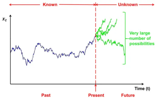
The handful of existing drowsiness monitoring systems based on the physiology of the monitored individual generally use data acquired in a window of time that is a few (tens of) seconds long and extends up to close to the present time. This means that the LoD values produced do not correspond to the present time, but to a time in the recent past, which can be, say, 20 or 30 seconds in the past. When one realizes that it only takes two (2) seconds for a typical vehicle to leave its driving lane and possibly hit a nearby fixed or moving obstacle, one immediately realizes the interest and importance of estimating, at the present time, what the LoD will be even in a time as short as two (2) seconds in the future. Of course, it is also very useful to make LoD-related predictions farther into the future. Hence, prediction is crucial for operational, real-time drowsiness monitoring systems.

We examined the two prediction frameworks of random process (RP) mod-els and machine learning (ML) techniques. However, we ultimately reached the conclusion that the use of RP models was more feasible to make LoD-related pre-dictions.

Given their nature, LoD signals must be viewed as realizations of RPs. Within the context of RPs, predicting the (unknown) future values (FVs) of such signals, as well as related events, based upon data available up to close to the present time

(4)

dently of any drowsiness monitoring system, it is also intellectually interesting to try to further understand what biological and physiological process underlie the evolution in time of LoD signals, and, more generally, of drowsiness.

The RP models that often come to mind in a wide variety of applications are the AR, MA, ARMA, and ARIMA RP models, where ”AR” stands for ”autore-gressive”, ”MA” for ”moving average”, and ”I” for ”integrated”. We examine the application of these conventional RP models to LoD signals, and we find that these signals can be properly modeled by AR(I)MA RP models. However, we also point out that these conventional RP models are quite heavy to deal with, and require human intervention in the process of building the RP models; it follows that they are not suitable for real-time applications.

Our search for better RP models in the context of drowsiness monitoring led us to examine the geometric Brownian motion (GBM) RP model. This RP model is frequently used in finance and led to two Nobel prizes in Economic Sciences, i.e., to Professor Paul Samuelson (MIT) in 1970, and to Professor Robert Merton and Professor Myron Scholes (Stanford and MIT) in 1997. However, the GBM RP model is generally unknown in other important domains, such as in engineering.

Using a carefully planned and executed protocol, and a validated drowsiness monitoring system, we collected discrete-time signals that represent the evolu-tion of the LoD of 30 individuals at three progressively increasing levels of sleep deprivation over three days, thus resulting in 90 validated LoD signals.

We showed that GBM is a valid choice of RP model for modeling all 90 LoD signals, thus without a single exception. Of course, the GBM RP model corre-sponding to each of the 90 signals is characterized by a set of parameters specific to this signal.

We stress that a given GBM RP model can model a signal/realization with a trend that is mostly either growing, or steady-state, or decreasing (and only one such trend). The fact that the 90 signals examined are relatively short (9.2 or 14 minutes) explains why a single (i.e., fixed) GBM RP model has a chance to model them successfully. As already alluded to, for longer signals (say, of 1 or more hours), it is critical to adapt the GBM model with time. We studied the question of adaptation from several points of view, and we suggested a pragmatic approach consisting in using a sliding time window and recomputing the parameters of the model using the sample in each successive window.

Besides the modeling of LoD (and PERCLOS) signals via the GBM RP model (either fixed or adaptive), we developed in detail methods of predictions (of futures values and other statistical parameters), and we applied them to a number of the

(5)

ventional RP models. We observed that the GBM RP model provides the same accuracy as the best conventional RP models, but with a computation time re-duced by a factor of 1,000.

We developed several drowsiness-prediction systems, and we considered and evaluated in detail one of them (based on the concept of survival probability).

In conclusion, the time-adaptive GBM RP model appears to be particularly well suited for modeling LoD signals and related signals such as the PERCLOS signals, and its application in drowsiness monitoring systems could lead to the development of operational systems with far greater capabilities of preventing accidents due to falling asleep at the wheel and, thus, of saving human lives.

(6)

First and foremost, I would like to express my sincere gratitude to my supervisor Prof. Jacques G. Verly for his continuous support of my PhD studies and research, for his patience, motivation, enthusiasm, and immense knowledge. His guidance helped me in my research and my personal life. I enjoyed every single second of working with him, and I could not have imagined having a better advisor. I will be forever grateful to him for having given me the opportunity to realize my thesis under his supervision.

Besides my advisor, I would like to thank the other members of my thesis committee, namely, Prof. Maarten Arnst, Dr. Cl´ementine Fran¸cois, Dr. Quentin Massoz, Prof. Jean-Michel Redoute, and Prof. Louis Wehenkel for accepting to be on the jury of this PhD thesis and for providing several valuable comments on some first drafts of this document.

I wish to thank particularly Dr. Cl´ementine Fran¸cois, for many years on our research team, for providing the level-of-drowsiness signals used in this thesis. She played a significant role in their acquisition, as part of her own PhD thesis work.

My sincere thanks goes to my friends and colleagues from the University of Li`ege, including, Quentin, Artem, Evgeny, Elizaveta, Marie, Sampath, Andreas, Kirill, Sude, Justinas, Yuan, Irien, and Stephan.

Last but not the least, I would like to thank my mother Nasrin, my father Houshang, and my brother Pedram, for their unconditional love and support.

(7)

1 Introduction 1

1.1 Context . . . 1

1.2 Goals of thesis . . . 2

1.3 Personal contributions . . . 3

1.4 Brief descriptions of subsequent chapters . . . 5

1.5 Remark . . . 8

2 Drowsiness: medical basis and characterization systems 9 2.1 Introduction . . . 9

2.2 Sleep and drowsiness . . . 10

2.2.1 Sleep mechanism . . . 11 2.2.1.1 Circadian process . . . 11 2.2.1.2 Homeostatic process . . . 12 2.2.1.3 Two-process model . . . 12 2.2.2 Sleep disorders . . . 13 2.2.2.1 Insomnia . . . 14

2.2.2.2 Excessive Daytime Sleepiness (EDS) . . . 14

2.2.2.3 Obstructive sleep apnea . . . 15

2.2.2.4 Narcolepsy . . . 15

2.2.3 Drowsiness. . . 16

2.2.3.1 Definition of drowsiness . . . 16

2.2.3.2 Difference between drowsiness and fatigue . . . 16

2.3 Clinical methods for characterizing drowsiness . . . 17

(8)

2.3.2.1 Multiple Sleep Latency Test (MSLT) . . . 18

2.3.2.2 Maintenance of Wakefulness Test (MWT) . . . 19

2.3.2.3 Oxford Sleep Resistance (OSLER) test . . . 20

2.4 Methods for characterizing drowsiness in operational settings . . . . 20

2.4.1 Subjective methods . . . 20

2.4.1.1 Karolinska Sleepiness Scale (KSS). . . 20

2.4.1.2 Stanford Sleepiness Scale (SSS) . . . 22

2.4.1.3 Visual Analog Scale (VAS) . . . 22

2.4.2 Objective methods . . . 22

2.4.2.1 Physiology-based methods . . . 22

2.4.2.1.1 Polysomnography (PSG) . . . 23

2.4.2.1.2 Ocular parameters (OPs) . . . 23

2.4.2.1.3 Facial expressions . . . 24

2.4.2.1.4 Skin conductance . . . 24

2.4.2.1.5 Heart rate (HR) . . . 24

2.4.2.2 Performance-based methods . . . 25

2.4.2.2.1 Psychomotor Vigilance Test (PVT) . . . . 25

2.4.2.2.2 Johns Test of Vigilance (JTV) . . . 25

2.4.2.2.3 Driving performance . . . 25

2.5 System used to produce level-of-drowsiness data for later experiments 26 2.6 Basic motivation for need for prediction. . . 26

2.7 Conclusion . . . 27

3 Prediction 28 3.1 Introduction . . . 28

3.2 General principle of prediction in our work . . . 29

3.3 Types of predictions . . . 33

3.3.1 Review of key elements of survival analysis (SA) . . . 34

3.3.1.1 Follow-up . . . 34

3.3.1.2 Event . . . 34

(9)

3.3.1.6 Hazard function . . . 37

3.3.1.7 Cox model . . . 38

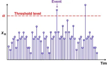
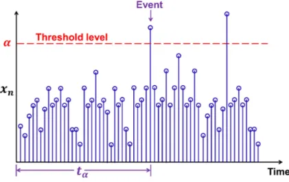
3.3.2 Casting prediction problem as a survival-analysis problem . 39 3.3.2.1 “Event” defined as first passage through some thresh-old level . . . 39

3.3.2.2 First hitting time (FHT) . . . 40

3.4 Prediction using random processes models . . . 40

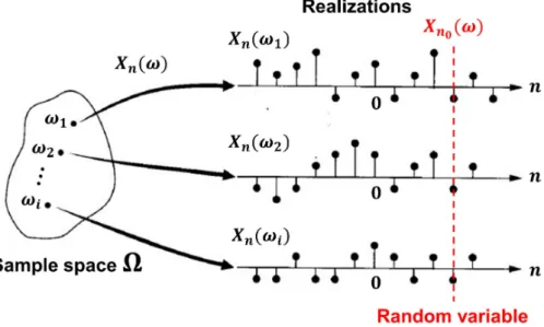
3.4.1 Brief introduction to random processes (RPs) . . . 40

3.4.2 Predicting future values of a signal using RP models . . . . 42

3.4.3 Predicting “first hitting time” and “survival probability” us-ing RP models . . . 44

3.5 Prediction using machine learning techniques . . . 45

3.5.1 Brief introduction to machine learning (ML) . . . 45

3.5.2 Predicting future values of a signal using ML techniques . . 46

3.5.3 Predicting “first hitting time” and “survival probability” us-ing ML techniques . . . 48

3.6 Random process models as an appropriate framework for prediction 48 3.6.1 Goal of prediction. . . 49

3.6.2 Available amount of data (aka cost) . . . 49

3.6.3 Accuracy of prediction (aka performance). . . 50

3.6.4 Complexity . . . 50

3.6.5 Final choice of framework . . . 51

4 Random processes and related models 53 4.1 Introduction . . . 53

4.2 Random processes (RPs) . . . 54

4.2.1 Discrete-time random processes (DT RPs) . . . 54

4.2.2 Continuous-time random processes (CT RPs) . . . 55

4.2.3 Remarks . . . 55

4.2.4 Key concepts . . . 55

(10)

4.2.4.4 Case of zero mean . . . 60

4.2.4.5 Computation of moments . . . 60

4.2.4.6 Notation. . . 60

4.2.4.7 Partial autocorrelation function (PACF) . . . 60

4.3 Conventional RP models . . . 61

4.3.1 White noise (WN) RP . . . 61

4.3.2 Autoregressive (AR) RP . . . 61

4.3.3 Moving average (MA) RP . . . 62

4.3.4 Autoregressive moving average (ARMA) RP . . . 63

4.3.5 Autoregressive integrated moving average (ARIMA) RP . . 63

4.4 Geometric Brownian motion (GBM) RP model . . . 64

4.4.1 Wiener process . . . 64

4.4.1.1 Discrete-time Wiener process . . . 65

4.4.1.2 Continuous-time Wiener process . . . 66

4.4.1.3 A word about notation “dWt” . . . 66

4.4.2 Itˆo process . . . 67

4.4.2.1 Drifted Brownian motion . . . 67

4.4.2.2 Geometric Brownian motion (GBM) . . . 68

4.4.3 History and interpretation . . . 70

5 Prediction using conventional random process models 73 5.1 Introduction . . . 73

5.2 Box-Jenkins method . . . 74

5.2.1 Selection of RP model and of its order . . . 74

5.2.2 Estimation of parameters of RP model . . . 74

5.3 Prediction using conventional RP models . . . 76

5.3.1 Predicting future values of a signal using conventional RP models . . . 77

(11)

5.4 Weaknesses of Box-Jenkins method . . . 78

6 Prediction using GBM random process model 80 6.1 Introduction . . . 80

6.2 Validation of GBM assumption: checking normality and indepen-dency conditions . . . 81

6.2.1 Techniques for checking normality condition . . . 82

6.2.1.1 Histogram . . . 82

6.2.1.2 Quantile-quantile (Q-Q) plot . . . 82

6.2.1.3 Shapiro-Wilk (S-W) test . . . 83

6.2.2 Techniques for checking independency condition . . . 83

6.2.2.1 Linear regression . . . 83

6.3 Estimation of parameters of GBM RP model . . . 84

6.4 Prediction using GBM RP model . . . 84

6.4.1 Predicting future values of a signal using GBM RP model . 84 6.4.2 Predicting “first hitting time” and “survival probability” us-ing GBM RP model . . . 85

6.5 Advantages of the GBM RP model over the conventional RP models 86 6.6 Powerful strategy for finding the best possible RP model . . . 86

7 Collection of experimental data 89 7.1 Introduction . . . 89 7.2 Participants . . . 89 7.3 Protocol . . . 90 7.4 Instruments . . . 91 7.5 Measurements . . . 92 7.6 About Study C . . . 92 7.7 Conclusion . . . 92

(12)

8.2 Possible solutions for adaptation . . . 95

8.3 Looking ahead. . . 98

8.4 Pragmatic solution for adaptation . . . 99

8.5 Novel interpretation of proposed solution for adaptation. . . 99

8.6 Real-time checking of validity of GBM hypothesis in a window . . . 100

8.7 Limitations due to shortness of signals available to us . . . 101

8.8 Supporting experiment on synthetic data . . . 102

8.9 About the relation between a GBM signal and portions thereof. . . 108

8.9.1 First argument . . . 108

8.9.2 Second argument . . . 109

8.10 Further exploration of issue of normality . . . 109

8.10.1 Setting up of problem . . . 109

8.10.2 Sample mean and sample variance of drawn samples. . . 110

8.10.3 Hypothetical distribution of drawn samples. . . 111

8.10.4 Important property of sample-mean RV of drawn samples. . 112

8.10.5 Important property of the sample-variance RV of drawn sam-ples. . . 113

8.11 Application of results to problem of interest . . . 117

8.12 View and practice in finance . . . 118

8.13 Conclusions . . . 118

9 Experimental results for collected drowsiness-related signals: (1) modeling 121 9.1 Introduction . . . 121

9.2 Modeling of LoD & PERCLOS signals using GBM RP model for signals from Study A . . . 122

9.2.1 Level-of-drowsiness (LoD) signals . . . 122

9.2.1.1 Application of methodology to one example signal from Study A (“Signal A”) . . . 123

9.2.1.1.1 Check of normality condition . . . 123

9.2.1.1.2 Check of independency condition . . . 125

(13)

9.2.1.2.3 Conclusion for all 51 LoD signals from Study A . . . 127

9.2.1.2.4 Discussion of issue with Shapiro-Wilke (S-W test) . . . 127

9.2.2 PERCLOS signals . . . 129

9.2.2.1 Check of normality condition . . . 129

9.2.2.2 Check of independency condition . . . 129

9.2.2.3 Conclusion for all 51 PERCLOS signals from Study A129 9.2.3 Discussion of results for Study A . . . 129

9.3 Modeling of LoD & PERCLOS signals using GBM RP model for signals from Study B . . . 129

9.3.1 Level-of-drowsiness (LoD) signals . . . 130

9.3.1.1 Application of methodology to one example signal from Study B (“Signal B”) . . . 130

9.3.1.1.3 Conclusion for Signal B . . . 132

9.3.1.2 Results for all 39 LoD signals from Study B . . . . 133

9.3.1.2.3 Conclusion for all 39 LoD signals from Study B . . . 133

9.3.2 PERCLOS signals . . . 134

9.3.2.1 Check of normality condition . . . 134

9.3.2.2 Check of independency condition . . . 135

9.3.2.3 Conclusion for all 39 PERCLOS signals from Study B135 9.3.3 Discussion of results for Study B . . . 135

9.4 Illustration of computation of parameters of GBM RP model . . . . 135

9.5 Adaptation with time of GBM RP model . . . 136

9.5.1 Review of key points of Chapter 8 . . . 136

(14)

9.5.4 Second illustrative example of adaptation for one example signal from Study B . . . 139

9.5.5 Conclusion. . . 142

9.6 Modeling of LoD signals using conventional RP models . . . 142

9.6.1 Application of Box-Jenkins method to four example LoD signals from Study A . . . 143

9.6.2 Application of Box-Jenkins method to 51 LoD signals from Study A . . . 145

9.7 About modeling for signals from Study C . . . 145

10 Experimental results for collected drowsiness-related signals: (2)

prediction 147

10.1 Introduction . . . 147

10.2 Non-adaptive prediction of future values of a signal (for LoD signals)148

10.2.1 Illustration of non-adaptive prediction of future values of a signal using GBM RP model (for one LoD signal from Study A) . . . 148

10.2.2 Performance in prediction error and computation time . . . 149

10.2.2.1 Performance of GBM RP model for non-adaptive prediction of future values of a signal (for all 51 LoD signals from Study A) . . . 149

10.2.2.2 Performance of the conventional RP models for non-adaptive prediction of future values of a sig-nal (for all 51 LoD sigsig-nals from Study A) . . . 151

10.2.2.3 Comparison of performance of the GBM and the conventional RP models . . . 151

10.2.3 Discussion of results . . . 152

10.3 Adaptive prediction of future values (FVs) of a signal (for LoD signals)153

10.3.1 Illustration of adaptive prediction of FVs (for one signal from Study A) . . . 153

(15)

10.4.2 Second illustration of adaptive prediction of FHT (for one

signal from Study B) . . . 158

10.5 Adaptive prediction of survival probability (SP) (for LoD signals) . 160 10.5.1 First illustration of adaptive prediction of SP (for one signal from Study A) . . . 160

10.5.2 Second illustration of adaptive prediction of SP (for one sig-nal from Study B) . . . 162

10.6 Detection of drowsiness . . . 163

10.6.1 General principle of detection using a threshold . . . 163

10.6.2 Ground truth for evaluation of performance . . . 164

10.6.3 Key statistics describing the performance of a binary classifier165 10.6.4 Confusion matrix . . . 167

10.6.5 Receiver operating characteristic (ROC) curve . . . 167

10.6.6 Three adaptive drowsiness-detection systems using a threshold168 10.6.7 Illustration of adaptive detection of drowsiness based on SP 170 10.6.7.1 First illustration of adaptive detection of drowsi-ness based on SP (for one signal from Study A) . . 170

10.6.7.2 Second illustration of adaptive detection of drowsi-ness based on SP (for one signal from Study B) . . 171

10.6.8 Performance of adaptive drowsiness detection system based on SP . . . 172

10.6.8.1 Principle of detection. . . 172

10.6.8.2 Key detection statistics . . . 173

10.6.8.3 ROC curve with SP as parameter (for all 51 signals from Study A) . . . 174

10.6.8.4 ROC curve with SP as parameter (for all 39 signals from Study B) . . . 175

10.6.8.5 Comparison of ROC curves for Study A and Study B176 10.6.9 Discussion of results . . . 177

(16)

11 Conclusion 180

Publications 184

(17)

APA American Psychiatric Association AR AutoRegressive

ARIMA AutoRegressive Integrated Moving Average ARMA AutoRegressive Moving Average

ASP Average Sleep Propensity BJ method Box-Jenkins method BM Brownian Motion

CDC Centers for Disease Control and Prevention CDF Cumulative Density Function

DT Discrete Time ECG ElectroCardioGram

EDS Excessive Daytime Sleepiness EEG ElectroEncephaloGram EMG ElectroMyoGram EOG ElectroOculoGram ESS Epworth Sleepiness Scale FHT First Hitting Time FIR Finite Impulse Response FoS First-order Stationary

(18)

GBM Geometric Brownian Motion IIR Infinite Impulse Response

IR InfraRed

JVT Johns Test of Vigilance KSS Karolinska Sleepiness Scale LoD Level of Drowsiness

LR Log-Ratio

MA Moving Average

MSLT Multiple Sleep Latency Test MWT Maintenance of Wakefulness Test

NHTSA National Highway Traffic Safety Administration NTSB National Transportation Safety Board

OOG OptoOculoGraphy OSLER Oxford Sleep Resistance PDF Probability Density Function POG PhotoOculoGraphy

Process C Circadian process Process S Homeostatic process PSG PolySomnoGraphy

PVT Psychomotor Vigilance Test Q-Q Quantile-Quantile

RP Random Process RV Random Variable

(19)

SDE Stochastic Differential Equation SL Sleep Latency

SoS Second-order Stationary SP Survival Probability SSS Stanford Sleepiness Scale ST Sleep Threshold

SWGN Standard White Gaussian Noise S-W test Shapiro-Wilk test

WN White Noise WP Wiener Process

(20)

Introduction

1.1 Context

Drowsiness is a major cause of accidents in many areas of human activity (whether personal or professional), and transportation is probably the single most impor-tant source of drowsiness-related accidents. For example, one third (1/3) of fatal accidents on highways in France are reported due to the driver falling asleep at the wheel [6].

The large number of such driving accidents is due to the combined sheer number of road vehicles and the fact that, until recently, car manufacturers and safety authorities have taken no drastic, effective actions to prevent these accidents (even though they are generally preventable). Any driver—whether healthy or suffering from some sleep pathology—may become the victim of such an accident. These accidents typically result in severe injuries, deaths, and/or loss of property.

It is thus critical to monitor a driver’s level of drowsiness (LoD), and to devise in-car safety systems to help prevent drowsiness-related accidents. In 2019, the European Union (EU) Parliament adopted rules requiring life-saving technologies in vehicles. Starting in May 2022, all road vehicles sold in the EU will need to be fitted with safety systems including for drowsiness monitoring and intelligent speed assistance [44].

For road vehicles, it is useful to distinguish between three categories of in-vehicle systems for monitoring drowsiness, namely systems monitoring the car behavior (e.g., lane crossing), systems monitoring the driver behavior (e.g., steer-ing wheel motion), and systems monitorsteer-ing the driver physiology. The systems in the first category do not work when lane-separating (”white”) lines are not present or are covered, e.g., by snow, and have difficulties in curving roads. The systems

(21)

in the first two categories are specific to road vehicles and not transferable to air, water, and space vehicles. The systems in the last category are the only ones that can truly measure the state of drowsiness of a person, and they are applica-tion independent and ”universal”. They can also be used outside the domain of transportation.

To the best of our knowledge, the handful of existing drowsiness monitoring systems based on the physiology of the monitored person use data acquired in a time window that is a few (tens of) seconds long and extends up to close to the present time. This means that the LoD values that these systems produce do not even correspond to the present time, but to a time in the recent past, which can be, say, 20 or 30 seconds in the past.

When one realizes that it only takes two (2) seconds for a vehicle moving at 96 km/h (60 mph) to leave its driving lane and possibly hit a nearby obstacle, one immediately understands the interest and importance of estimating, at the present time, what the LoD will be even in two (2) seconds [26]. Of course, it is also very useful to make LoD-related predictions farther into the future. Hence, prediction is crucial for operational, real-time drowsiness monitoring systems.

1.2 Goals of thesis

All significant drowsiness monitoring systems that reasonably claim to estimate and produce the LoD of an operator in real-time do, in fact, produce an LoD that is representative of the recent past and not of the present time. Even if this LoD did somehow correspond to the present time, it might be too late to take proper action to avoid an accident. Therefore, there is an imperative need to estimate how the LoD will evolve past the present time, and to make various types of predictions based on the past evolution of the LoD with time. These LoD-related predictions can take several forms, such as predicting future values (FVs) of the LoD, e.g., to anticipate the crossing of a reference (danger) level, or computing other quantities indicating a probability or risk of some event (happening). While this event might be ”leaving the driving lane”, one may wish to define other types of events that are intrinsically linked to the evolution of the LoD of a person, and not to a specific application such as driving.

The main goals of this thesis are as follows:

1. Design a system to predict, at the present time (”now”), the future evolution of the level of drowsiness (LoD) of a subject (e.g., a driver) based upon a number of ”measurements” taken (in some way) from this subject, preferably

(22)

non-invasively, which means, in the present context, without having to attach sensors (such as electrodes) to the subject.

2. Design other systems to produce other types of LoD-related predictions, e.g., the probability of some event (happening) or the time until the LoD crosses a reference (danger) level.

3. Provide an interpretable mathematical model for the evolution of drowsiness in time. Indeed, being able to show that the drowsiness of a person evolves according to a particular mathematical model would be a major contribution to basic science.

One should note that the problem of predicting FVs (of a signal) based upon past and present values is an important, classical problem of signal processing. Predicting FVs is absolutely essential in a number of applications, such as the compression of audio and video signals and the prediction of future stock prices. However, such predictions have not been investigated in the field of drowsiness monitoring. The main goal of the present thesis is to provide the missing link of prediction in the domain of technologies for drowsiness monitoring.

Figure 1.1 shows a typical drowsiness monitoring system and the position of the prediction subsystem in the processing chain. This subsystem is the main object of this thesis.

Figure 1.1: Block-diagram of a typical drowsiness monitoring system. The ”predict” subsystem is the main object of this thesis.

1.3 Personal contributions

This thesis contains the following main personal contributions:

• Identify the need, in drowsiness monitoring, to make predictions related to the evolution of the level of drowsiness (LoD) in the future.

(23)

• Identify the need to have a model (of some sort) of the past evolution of this LoD to enable the making of predictions.

• Participate in the collection of data to produce LoD signals of subjects per-forming specific tasks.

• Identify two candidate frameworks for modeling LoD signals, namely random process (RP) models and machine learning (ML) techniques.

• Perform an intensive investigation of the applicability to LoD signals of two types of RP models, namely (1) the geometric Brownian motion (GBM) RP model and (2) conventional RP models, i.e., autoregressive (integrated) moving average (ARIMA) models.

• Discover that the GBM RP model appears to be an excellent tool to model the local evolution of LoD signals.

• Identify the need for locally adapting the RP model, and thus of the impor-tant GBM RP model.

• Push as far as possible a theoretical analysis of the question of adaptation of the GBM RP model, discover that the ˆIto-process model (which is more general than the GBM RP model), while going in the right direction, is not general enough for our modeling needs.

• Propose the pragmatic solution of locally adapting the GBM RP model using a sliding time window (butting against the present time) and estimating the model parameters based on the samples in this window.

• Explore ways of performing various types of predictions for RP models, both GBM and conventional.

• Get the idea of bringing in concept from survival analysis.

• Develop as much as possible three types of predictions for above RP models: future values (FVs) (of LoD signal), the first hitting time (FHT), and the survival probability (SP).

• Develop drowsiness-detection systems based on the idea of thresholding FV, FHT, or SP signal, fully develop such a system based on SP, and evaluate its performance.

• Participate in a confidential study with a Belgian company and a major car manufacturer.

(24)

• Present at several national and international conferences, and publish results in various forms.

• Obtain several patents, with some pending, on the modeling and predic-tion using the GBM RP model and the ˆIto-process model in the context of drowsiness monitoring.

The main results of this thesis were published in journals, conference proceed-ings, and patents. Several results were also presented at conferences. The list of our publications is given near the end of the thesis.

1.4 Brief descriptions of subsequent chapters

The topics addressed in the next ten chapters of the thesis are as follows:

• Chapter 2

◦ motivates the work of the thesis by providing statistics on drowsiness-related accidents;

◦ describes the tightly-coupled phenomena of sleep and drowsiness, the biological mechanism of sleep, and sleep disorders;

◦ provides a clear definition of drowsiness, and explains the difference with fatigue;

◦ gives the main clinical methods for characterizing drowsiness, both sub-jective and obsub-jective;

◦ gives the main methods for characterizing drowsiness in operational settings;

◦ describes the system we used to produce signals characterizing the level of drowsiness.

• Chapter 3

◦ describes why prediction is absolutely necessary;

◦ provides detailed information about the main frameworks to produce LoD-related predictions;

◦ presents different types of LoD-related predictions;

◦ explains how to select an appropriate framework to produce LoD-related predictions.

(25)

• Chapter 4

◦ explains why LoD signals must be treated as realizations of an under-lying RP;

◦ provides the precise definition of a RP;

◦ presents the conventional RP models and the geometric Brownian mo-tion (GBM) RP model, which is the cornerstone of this thesis.

• Chapter 5

◦ describes how to use conventional RP models to produce different types of predictions;

◦ presents a method called the Box-Jenkins method to select an appro-priate conventional RP model for a given signal;

◦ addresses the main weaknesses of the Box-Jenkins method. • Chapter 6

◦ describes how to use the GBM RP model to produce different types of predictions, i.e., future values (FVs), first hitting time (FHT), and survival probability (SP);

◦ presents the methodology that is typically used to determine whether the GBM RP model is a valid RP model for a given signal;

◦ explains how to estimate the parameters of a GBM RP model;

◦ provides a list of the advantages of the GBM RP model over conven-tional RP models.

• Chapter 7

◦ provides an introduction to the laboratory-based experiments used in this thesis;

◦ describes the general characteristics of the participants, applied proto-cols, measurements setup, and drowsiness monitoring system used in our experiments.

• Chapter 8

◦ explains the need for adapting the RP model with time to properly handle long signals;

(26)

◦ emphasizes the fact that the GBM RP model can model a trend that is either growing, steady-state, or decaying (but not all at once), with the consequence that the model must be adapted to deal with long periods of time, such as for long drives;

◦ pushes as far possible, based upon the state of our knowledge, the theory of adaptation of the GBM RP model;

◦ addresses the question of whether a contiguous portion of a signal/realization that is GBM is also GBM;

◦ provides a pragmatic method for adapting the GBM RP model using a sliding time-window.

• Chapter 9

◦ describes the modeling results obtained from the experimental data (i.e., from laboratory-based experiments);

◦ illustrates the application of the methodology (presented in Chapter 6) to data obtained from laboratory-based experiments;

◦ illustrates the modeling of LoD signals using the GBM RP model; ◦ illustrates the modeling of LoD signals using the conventional RP

mod-els;

◦ illustrates the adaptation with time of the GBM RP model. • Chapter 10

◦ illustrates the non-adaptive prediction of FVs of an LoD signal using the GBM RP model;

◦ quantifies the performance of non-adaptive prediction of FVs (of a sig-nal) using both the GBM RP model and conventional RP models, this in terms of prediction accuracy and computation speed;

◦ illustrates the computation of the FHT and SP using a GBM RP model that adapts at each time step;

◦ describes drowsiness-detection systems built by applying a threshold to FVs, the FHT, and the SP;

◦ indicates how the detection of these systems can be characterized; ◦ describes in detail a drowsiness-detection system based on SP and

de-scribes its performance in terms of ROC curves. • Chapter 11

◦ summarizes the thesis and provides a perspective for possible future researches.

(27)

1.5 Remark

Throughout the thesis, we often use the gender-neutral terms ”he”, ”him”, and ”his”, which thus include the corresponding ”she”, ”her”, and ”her”.

(28)

Drowsiness: medical basis and

characterization systems

This chapter describes (1) the medical basis of drowsiness and (2) systems to char-acterize this drowsiness. Section 2.1 provides an introduction to drowsiness and drowsiness-related accidents. Section 2.2 describes the mechanisms of sleep and drowsiness. Section 2.3provides an overview of the clinical methods used for char-acterizing drowsiness. Section 2.4 describes the methods used for characterizing drowsiness in operational settings. Section 2.5 presents the system used to pro-duce level-of-drowsiness data in our laboratory-based studies. Section 2.6 gives the basic motivation for making predictions in the context of drowsiness. Section 2.7

concludes this chapter.

2.1 Introduction

The drowsy state is an intermediate state between alert wakefulness and sleep [1, 53, 54, 55]. Drowsiness is a major cause of accidents in many areas of human activity (whether personal or professional), and transportation is probably the single most important source of drowsiness-related accidents.

According to one study in France, one third (1/3) of fatal accidents on highways are reported to be due to the driver falling asleep at the wheel [6].

Another study in the United States (US) shows that drowsy driving between 2009 and 2013 led to an estimated 21% of crashes resulting in death and to an estimated 13% of crashes causing severe injury [66].

In 2013, in the US, the ”National Highway Traffic Safety Administration (NHTSA)” estimated that drowsy driving was responsible for 72,000 crashes, 44,000 injuries,

(29)

and 800 deaths [78]. However, according to the ”Centers for Disease Control and Prevention (CDC),” these numbers are underestimated, and drowsiness leads to nearly 6,000 fatal crashes every year [17].

Furthermore, the risk of drowsy driving is more important for those who work during the night, e.g., police officers and firefighters. In the US, about 15% of workers, i.e., over 15 million people, work the night shift or rotating shift schedules [68].

Drowsiness in police officers has been reported ”to significantly increase the number of errors, safety violations, injuries, and falling asleep while driving” [70]. According to one study in the US, ”28.5% of police officers surveyed reported falling asleep while driving at least once a month” [70].

Despite the large number of drowsiness-related accidents, drowsy driving is often referred to as a preventable public health issue [68]. It is thus paramount to monitor the level of drowsiness (LoD) of a driver and to devise in-car safety systems that can help prevent often-catastrophic accidents due to drowsiness.

In the next section, we provide an overview of sleep and drowsiness, which are intertwined topics.

2.2 Sleep and drowsiness

Sleep is a biological imperative that appears to be evolutionarily preserved under the influence of the natural selection process operating across species [43]. As a consequence of the shared evolutionary history between humans and other species, sleep became a biological imperative for humans [43].

Sleep is essential for the human body to maintain good functioning and health. In fact, sleep of sufficient duration, continuity, and intensity (depth) is necessary to promote high levels of attention and cognitive performance during the wake period, and to prevent physiological changes with adverse health outcomes in general [43,

38].

The need to sleep increases with the duration of wakefulness and dissipates with time spent asleep [88]. Drowsiness is the intermediate state between (1) wakefulness and (2) sleep. In the same vein as hunger and thirst are the instincts that drive us to eat and drink, drowsiness is the instinct that drives us to sleep [38]. Therefore, drowsiness and sleep are inextricably intertwined topics.

This section comprises three subsections. The first two subsections provide a reasonably comprehensive overview of the sleep mechanism and sleep disorders, and the third subsection provides a theoretical introduction to drowsiness.

(30)

2.2.1 Sleep mechanism

It is generally agreed that our sleep-wake pattern and our alertness level during wakefulness can be explained by a two-process model. The two processes of the model are (1) the homeostatic process (denoted by S), which corresponds to the drive for sleep that increases as we stay awake and decreases when we sleep, and (2) the circadian processes (denoted by C), which corresponds to the internal oscillatory rhythm that has a period of about 24 hours and can be reset by the environmental light [33, 43].

One should note that this two-process model has probably been the most domi-nant model in the field of sleep over the past 30 years, in part because the concepts of the model are easy to apply to a broad range of questions in sleep research [25]. In subsequent subsections, we first introduce the homeostatic and circadian processes, and we then explain how these two processes work together.

2.2.1.1 Circadian process

The drive for sleep increases as we stay awake and decreases when we sleep. When the drive for sleep reaches a certain threshold level, it triggers sleep. This threshold level fluctuates periodically in a 24h cycle, i.e., it has circadian fluctuations. In the context of the two-process model, this fluctuating threshold level is called the sleep threshold (denoted by ST). In the same vein as the sleep threshold, the wakefulness threshold (denoted by WT) is defined as a fluctuating threshold level that triggers wakefulness. The circadian fluctuations of the sleep and wakefulness thresholds are controlled by a biological clock. This mechanism is called the circadian process or simply process C [46].

The circadian fluctuations of the sleep and wakefulness thresholds (i.e., ST and WT) are shown inFigure 2.1 [46].

The circadian process is endogenous (i.e., internally generated), and consists in self-sustaining oscillations. Therefore, the circadian process continues periodically even in the absence of periodic external time cues, such as sunlight and darkness, or sleep and wakefulness.

In humans, many other physiological processes, such as body temperature, re-nal and cardiac function, and hormone secretion also vary according to a circadian process [29].

The circadian process is present at all levels of biological complexity from unicellular organisms to humans. The reason for this is that the origin of life on Earth, behavior, and physiology have been shaped by the rotation of our planet around its axis. Consequently, a biological circadian timing system evolved and

(31)

enabled species to anticipate daily environmental changes rather than just reacting to them [25,29].

2.2.1.2 Homeostatic process

The future sleep is affected by the duration of the current wakefulness. After prolonged wakefulness due, e.g., to staying up all night, there is an increase in the desire for sleep during the following day. The longer the duration of continuous wakefulness before sleep onset (i.e., the duration of sleep deprivation) is, the greater the sleep propensity is [46,38].

In human, sleep propensity or sleep pressure caused by prolonged wakefulness is called the homeostatic process, or simply process S [46].

To illustrate the evolution with time of the level of process S, we consider three cases over two full days (Day 1, Night 1, Day 2, Night 2):

1. Baseline case: each day, subject stays awake for 16 hours (Day 1 and Day 2) and sleeps 8 hours (Night 1 and Night 2).

2. 2-h nap case: same as baseline case, except for a 2-h nap around 6 pm on Day 1.

3. Sleep deprivation case: same as baseline case, except that subject is pre-vented from sleeping during Night 1.

Figure 2.1 shows the evolution of the level of process S over the two full days of interest for the three above cases [25].

2.2.1.3 Two-process model

The two-process model of sleep regulation was proposed by Borb´ely and Dann in 1982 [9,10]. This model is essential to understanding the relationship between the sleep-wake cycle and the biological-clock system in humans.

In the two-process model, as already described in Section 2.2.1.2, process S represents sleep homeostasis or sleep debt, which increases during waking and decreases during sleep, within a range that oscillates with a periodicity that is entrained by the circadian process (i.e., process C).

When S reaches the wakefulness threshold WT, it triggers wakefulness, and when S reaches the sleep threshold ST, it triggers sleep. The most important interactions between the two processes occur at the moments where S reaches the sleep threshold ST, transitioning from wakefulness to sleep, or the wakefulness threshold WT, transitioning from sleep to wakefulness.

(32)

A simplified representation of the two-process model of sleep regulation, for the three cases mentioned in Section 2.2.1.2 within a two-day period, is shown in

Figure 2.1.

Figure 2.1: The graph shows the evolution of the level of process S as a function of time over two full days divided in four successive parts, i.e., Day 1, Night 1, Day 2, Night 2, for three cases described in the text, and respectively corresponding to the baseline, 2-h nap, and sleep deprivation cases. The circadian fluctuations of the sleep threshold (ST) and wakefulness threshold (WT) are shown over the period of interest. This figure is strongly inspired from Figure 2 in [25].

2.2.2 Sleep disorders

As already alluded to, sleep of sufficient duration, continuity, and depth is essential for the human body to maintain good functioning and good health. According to the “American Psychiatric Association (APA)”, any problem associated with the quality, timing, and amount of sleep, is considered to be a sleep disorder [5]. In fact, sleep disorders can severely affect the cognitive performance of an individual during the wake period, and, consequently, his safety and quality of life. One should note that sleep disorders are linked to both physiological and emotional problems [5].

In subsequent subsections, we provide a brief introduction to some common sleep disorders.

(33)

2.2.2.1 Insomnia

Insomnia involves problems getting to sleep or staying asleep. According to the APA, insomnia is the most common sleep disorder. Indeed, roughly one-third of adults report some symptoms of insomnia. Furthermore, an estimated 40-50 percent of individuals with insomnia also suffer from some other mental disorders [5].

Problems in getting to sleep are more common among young adults and prob-lems in staying asleep are more common among middle-age and older adults. Some common treatments for improving quality of sleep are as follows:

• relaxation techniques before bedtime, • herbs and dietary supplements, and • melatonin supplements.

2.2.2.2 Excessive Daytime Sleepiness (EDS)

A person who has excessive daytime sleepiness (EDS) feels drowsy, i.e., affected by drowsiness (as defined in upcomingSection 2.2.3) everyday, and this symptom often interferes with his work, study, and daily activities. Although people with this condition often complain of ”fatigue” and of a general lack of energy, EDS is different from fatigue, which is characterized by low energy and the need to rest but not necessarily to sleep. EDS is also different from depression. Indeed, a person suffering from depression may have a reduced desire to do normal activities, even the ones he used to like [23, 38].

EDS is a common sleep disorder. Indeed, about 20% of the population can be classified as suffering from EDS.

Common causes are as follows:

• poor sleep habits,

• another sleep disorder, e.g., obstructive sleep apnea (described later), • side effects from certain medications, and

• other underlying medical conditions.

For most people suffering from EDS, changing their sleep habits and their sleep environments improves their conditions. For some people suffering from this condition, further medical tests and/or sleep studies are required [23].

(34)

2.2.2.3 Obstructive sleep apnea

A person with obstructive sleep apnea has repeated periods of breathing problems during sleep causing snoring or pauses in breathing. This interrupted sleep causes sleepiness during daytime. Sleep apnea is diagnosed with a clinical sleep study using as polysomnography (PSG) [5].

Sleep apnea affects about 2% to 15% of middle-age adults and more than 20% of older adults. The main risk factors for sleep apnea are as follows:

• obesity,

• male gender, and

• family history of sleep apnea.

2.2.2.4 Narcolepsy

Narcolepsy is a chronic sleep disorder, the exact cause of which is unknown. It is characterized by excessive and overwhelming daytime sleepiness, even after ade-quate nighttime sleep. A person with narcolepsy is likely to become drowsy (as defined later in Section 2.2.3) or to fall asleep, often at inappropriate times and places. The sleep attacks may occur with or without warning, and may be irre-sistible [81].

Other classic symptoms of narcolepsy are as follows:

• Cataplexy: sudden episodes of loss of muscle function, where this loss may vary from slight weakness to complete body collapse.

• Sleep paralysis: temporary inability to talk or move when falling asleep or waking up, where this inability may last from a few seconds to several minutes.

• Hypnagogic hallucinations: vivid, often frightening, dream-like experiences that occur while falling asleep.

Sleep paralysis and hypnagogic hallucinations can also occur in people who do not have narcolepsy. Narcolepsy affects 0.04% of the population, but it is estimated that less than 25% of affected people are diagnosed.

Narcolepsy is often misdiagnosed as being related to depression, epilepsy, and the side effects of medications [81].

(35)

2.2.3 Drowsiness

As already indicated, drowsiness and sleep are intertwined topics. In fact, drowsi-ness is a physiological necessity that drives us to sleep [38].

Below, we first provide a precise definition of drowsiness, and we then clarify the major differences between drowsiness and fatigue.

2.2.3.1 Definition of drowsiness

In the context of the work described in this thesis, it is of the utmost importance to provide a precise definition of drowsiness. One of the most precise and recent definitions of drowsiness is the one proposed by Q. Massoz [72]:

”Drowsiness is defined as the state of being drowsy, that is, having a difficulty of staying awake, a strong inclination toward falling asleep. Here follow the main characteristics of drowsiness:

• it is an intermediate state between fully awake and asleep; • it is experienced at a continuous level that varies in time;

• it is characterized by physiological changes, and by impairments of both cognitive performance, and psychomotor performance.”

One should note that, there is confusion among such terms as ”sleepiness”, ”drowsiness”, ”somnolence”, and ”fatigue” [55, p. 3]. In fact, the first three terms, i.e., ”sleepiness”, ”drowsiness”, and ”somnolence” are synonyms and can be used interchangeably [72, 38]. But, as already indicated in Section 2.2.2.2, ”fatigue” is significantly different from ”drowsiness”. Below, we clarify the key difference between ”drowsiness” and ”fatigue”.

2.2.3.2 Difference between drowsiness and fatigue

Concerning ”fatigue”, one must distinguish physiological or muscular fatigue from psychological or mental fatigue. Here, we talk about psychological/mental fatigue. Psychological fatigue is defined as the ”subjective experience of tiredness and a disinclination to continue performing the current task” [14, 55]. Fatigue is asso-ciated with the duration of a continuous task and the available time for rest (but not necessarily for sleep).

Clearly, the two concepts, i.e., ”drowsiness” and ”fatigue” have arisen from different disciplines. ”Fatigue” came from the psychology of work and performance, whereas ”drowsiness” came from the study of sleep [55, p. 6].

(36)

In a nutshell, fatigue refers to a feeling of tiredness or exhaustion due to per-forming a continuous task, whereas drowsiness refers to a physiological state be-tween alertness and sleep.

2.3 Clinical methods for characterizing

drowsiness

We provide a brief introduction to the clinical methods for characterizing drowsi-ness. For further details about each method, one can refer to [38].

Figure 2.2 shows a hierarchy of the clinical methods. The figure shows that the clinical methods for characterizing drowsiness fall into two broad categories: (1) subjective methods, which are mainly based on questionnaires and refer to self-reported measurements, and (2) objective methods, which are mainly based either on performance measures or on physiological measures [38, 72, 55].

Figure 2.2: Hierarchy of clinical methods for characterizing drowsiness. This figure is strongly inspired from Figure 2.2 in [38].

We now successively describe each of the two broad categories of methods, i.e., subjective and objective methods.

2.3.1 Subjective methods

The subjective methods are mainly based on questionnaires, which evaluate the sleep propensity based on the answers of the respondent.

Below, we provide an overview of the most common subjective method to evaluate sleep propensity in a clinical setting, i.e., the Epworth Sleepiness Scale (ESS).

(37)

2.3.1.1 Epworth Sleepiness Scale (ESS)

The Epworth Sleepiness Scale (ESS) test asks the respondent to score on a 4-point scale (0-3) his usual chances of having ”dozed off” or “fallen asleep” while engaged in eight different activities such as sitting and reading, watching TV, sitting and talking to someone, etc. These activities vary widely in their somnificity; e.g., a specific person falls asleep more easily when he is watching TV than when he is sitting and talking to someone [38, 56].

The total ESS score gives an estimate of “average sleep propensity (ASP)” of a person in his daily life [56].

The interpretation of the ESS scores is given in Table 2.1. Epworth Sleepiness Scale (ESS) Score Interpretation

0-5 Lower normal daytime sleepiness 6-10 Higher normal daytime sleepiness 11-12 Mild excessive daytime sleepiness 13-15 Moderate excessive daytime sleepiness 16-24 Severe excessive daytime sleepiness

Table 2.1: Interpretations of the scores of the Epworth Sleepiness Scale (ESS) [38, 56].

The ESS is highly reliable to evaluate the general (average) sleep propensity of a person. However, one should note that, since the ESS test is taken at one specific point in the time, typically in a clinical setting, the ESS score does not represent the true state of drowsiness of a person at any later time, e.g., in real-time during driving. [38, 56].

2.3.2 Objective methods

The objective methods determine the sleep propensity based either on performance measures or on physiological measures.

Below, we provide overviews of the most common objective methods to evaluate sleep propensity in a clinical setting.

2.3.2.1 Multiple Sleep Latency Test (MSLT)

The Multiple Sleep Latency Test (MSLT) is designed to measure how fast one person falls asleep in a dark and quiet environment during the day. MSLT is

(38)

a standard tool to diagnose different sleep disorders such as narcolepsy. The test relies upon the idea that the drowsier a person is, the faster this person falls asleep. The MSLT is administrated during daytime and consists of four to five sessions, with each session called a “nap”. Naps are separated by 2-h breaks. During each nap, the subject lies quietly in bed and tries to fall asleep. The test measures the time between “lights out” (with eyes closed) and the moment when the subject falls asleep. In any case, the subject is awaken after 20 minutes [38].

The mean of the measured times for all four or five naps is called the sleep latency (SL). The interpretation of SL is presented in Table 2.2.

Multiple Sleep Latency Test (MSLT) SL (min) Interpretation

SL<5 Severe drowsiness 5<SL<10 Moderate drowsiness

SL>10 Normal drowsiness

Table 2.2: States of drowsiness based on the value of sleep latency (SL) [38].

The moment when the individual falls asleep is determined from polysomnog-raphy (PSG) recordings. For further details about PSG and MSLT, one can refer to [38].

2.3.2.2 Maintenance of Wakefulness Test (MWT)

The Maintenance of Wakefulness Test (MWT) is designed to measure drowsiness during the day. It is also a reliable diagnostic tool to identify EDS for legal considerations, such as reinstating a driver’s license. Similar to MSLT, MWT also relies upon the idea that the drowsier a person is, the faster this person falls asleep. The test is administrated during daytime and consists of four sessions that are separated by 2-h breaks. For each session, the subject is asked to stay awake as long as possible. Each session ends when the subject falls asleep or after 40 minutes if he does not. During the test, the subject is isolated from outside factors that can affect his ability to fall asleep, e.g., the room should be quiet and dimly lit.

The mean of the durations between the start of the session and the moment the subject falls asleep is usually called the MWT SL.

In the same way as the MSLT, the moment when the individual falls asleep is determined from polysomnography (PSG) recordings.

(39)

The MWT latencies of less than 8 minutes may indicate an underlying sleep disorder such as EDS [38].

2.3.2.3 Oxford Sleep Resistance (OSLER) test

The Oxford Sleep Resistance (OSLER) test is very similar to the Maintenance of Wakefulness Test (MWT). The fundamental difference is that the OSLER test uses performance-based parameters to determine the moment when the individual falls asleep, whereas the MWT uses EEG-based parameters.

During the test, the individual is asked to lie down and to try to stay awake. He must respond to a light stimulus by touching a button. The light stimulus consists in a LED that flashes for one second every three seconds. To determine the SL for one 40 minutes session, the test measures the time before the occurrence of 7 consecutive flashes without any response (i.e., 21 seconds) [52].

There is good correlation between the results from the OSLER test and those of the MWT [38]. For further details about the OSLER test, one can refer to [38, 52].

2.4 Methods for characterizing drowsiness in

operational settings

In this section, we provide an overview of the main methods for characterizing drowsiness in real-time (aka operational methods). We divide the operational methods into two broad categories: (1) subjective methods, which are mainly based on questionnaires, interviews, or self-reports from the subject, and (2) objective methods, which are based on the direct measurement of physiological parameters of the subject or on the performance of the subject while performing a task.

Figure 2.3 shows a hierarchy of the operational methods.

2.4.1 Subjective methods

Below, we present three main subjective methods for characterizing the drowsiness of a person in an operational setting.

2.4.1.1 Karolinska Sleepiness Scale (KSS)

The Karolinska Sleepiness Scale (KSS) test measures the subjective level of drowsi-ness at a particular time during the day [86]. The test asks the respondent to select,

(40)

Figure 2.3: Hierarchy of operational methods for characterizing drowsi-ness. This figure is strongly inspired from Figure 2.3 in [38].

among nine drowsiness states (shown in Table 2.3), the one that best reflects his state of drowsiness in the last 10 minutes.

Karolinska Sleepiness Scale

Rating State

1 Extremely alert

2 Very alert

3 Alert

4 Rather alert

5 Neither alert nor sleepy 6 Some signs of sleepiness

7 Sleepy, but no effort to remain awake 8 Sleepy, some effort to stay awake

9 Very sleepy, great effort to stay awake, fighting sleep Table 2.3: Nine-point Karolinska Sleepiness Scale (KSS) [86,38].

Due to the simplicity of the test, it can be taken repeatedly without a major distraction to the respondent.

The KSS results are highly correlated with EEG features [86, 38, 57]. In part due to this correlation, the KSS is the most prevalent subjective scale in the drowsiness-related literature. However, the KSS test is not a reliable tool to diag-nose sleep disorders [38].

(41)

2.4.1.2 Stanford Sleepiness Scale (SSS)

The Stanford Sleepiness Scale (SSS) is very similar to the KSS. The main difference is that SSS uses a seven-point scale for characterizing drowsiness.

The SSS drowsiness states are shown in Table 2.4. Stanford Sleepiness Scale

Rating State

1 Feeling active, vital, alert, or wide awake

2 Functioning at high levels, but not at a peak; able to concentrate 3 Awake, but relaxed; responsive but not fully alert

4 Somewhat foggy, let down

5 Foggy; loosing interest in remaining awake; slowed down 6 Sleepy, woozy, fighting sleep; prefer to lie down

7 No longer fighting sleep, sleep onset soon; have dream-like thoughts Table 2.4: Seven-point Stanford Sleepiness Scale (SSS) [38].

2.4.1.3 Visual Analog Scale (VAS)

The Visual Analog Scale (VAS) is a tool used to help a subject rate the intensity of certain sensations and feelings, such as pain, satisfaction, or drowsiness.

The VAS for drowsiness is a horizontal straight line segment with two ends, corresponding to ”very alert” and ”very drowsy”. The subject is asked to mark a point on the scale/segment that reflects his level of drowsiness in the last few minutes. The position of the mark can then be converted into a number, e.g., from 0 to 10 [38].

2.4.2 Objective methods

Below, we provide an overview of the objective methods for charactering drowsiness in operational settings. These methods can be divided into two categories: (1) physiology-based methods, which are independent of the task performed by the subject, and (2) performance-based methods, which are dependent on this task.

2.4.2.1 Physiology-based methods

Below, we briefly introduce the five most common physiology-based methods for characterizing drowsiness in operational settings.

(42)

2.4.2.1.1 Polysomnography (PSG)

Polysomnography (PSG) is the gold standard for sleep studies. PSG simultane-ously records, via the use of electrodes, several body activities such as from the brain (via the electroencephalogram (EEG)), the eye (via the electrooculogram (EOG)), the muscles (via the electromyogram (EMG)), and the cardiac activity (via the electrocardiogram (ECG)) [58, 87, 38].

PSG is considered to be the gold standard for diagnosing many different sleep disorders [87]. In addition to this, since the late 90s, PSG signals have been used to determine the state of drowsiness of an individual in “active situations” (i.e., not necessarily laying down with closed eyes) and at a given time [38].

The Karolinska Drowsiness Scale (KDS) and the Objective Sleepiness Scale (OSS) are the main PSG-based methods for characterizing drowsiness in active situations.

In the KDS, one divides PSG signals into successive windows of 20 seconds and one visually determines a (KDS) score. The KDS score for each 20-second window varies from 0 (fully alert) to 100 (very drowsy).

Similarly to the KDS, the OSS also divides PSG signals into successive windows of 20 seconds and one visually determines the scores. However, the OSS scores vary from 0 (fully alert) to 4 (very drowsy).

For further details about the KDS and OSS scoring methods, one can refer to [38].

2.4.2.1.2 Ocular parameters (OPs)

The eyes are windows into the brain [65]. The activity of the eyes and their surrounding features (such as the eyelids) are closely related to cognitive processes (such as attention, memory, and decision-making), alertness or drowsiness, and, in general, brain activity [38].

In this thesis, we use the term ”ocular parameter (OP)” to denote a parameter that describes the state or dynamics of an eye and its surrounding area, including the eyelids.

To date, different OPs and their combinations have been proposed as reliable physiological markers of drowsiness [2, 27].

Among them, the PERCLOS (PERcentage of eye CLOSure) appears to have been the first OP to be widely recognized as a reliable measure for characterizing the level of drowsiness of a subject.

The PERCLOS is defined as percentage of time that the eye remains closed more than 80 (or 70) % [62,27].

(43)

The definition of PERCLOS was established for the first time in 1994 during a driving simulator study [62, 27]. Since then, several other OPs, such as the duration of blinks and their frequency, have demonstrated promising efficiency in the characterization of drowsiness.

There are three main techniques for extracting OPs: (1) photooculography (POG), based on the acquisition and analysis of video images of the eye, (2) optooculography (OOG), based on the transmission of infrared (IR) pulses and on the analysis of the reflected signals, and (3) electrooculography (EOG), based on the measuring the corneo-retinal dipole potential of the eyeball [38].

2.4.2.1.3 Facial expressions

Several studies have explored the link between ”facial expressions” and ”drowsi-ness” [73, 77]. Recent advances in computer-vision algorithms provide the op-portunity to monitor, in real-time, different drowsiness-related facial expressions, such as yawn, lip stretch, and eye blink. These facial expressions can be used for characterizing drowsiness, in real-time and non-invasively, in operational settings. For further details about the link between facial expressions and drowsiness, one can refer to [72,73, 77]

2.4.2.1.4 Skin conductance

The skin conductance—aka electrodermal activity (EDA)—is used to quantify the sweat gland activity and changes in the sympathetic nervous system. The EDA can be measured by two electrodes placed on the surface of the skin (typically on the palm or fingertips). Several studies propose EDA as a physiological marker of drowsiness [83, 38].

2.4.2.1.5 Heart rate (HR)

The heart rate (HR) is another physiological marker of drowsiness. One can divide the HR frequency spectrum into two parts: (1) the low-frequency (LF) part in the range of [0.04 − 0.15] Hz, and (2) the high-frequency (HF) part in the range of [0.15 − 0.4] Hz. Some studies have shown that the ratio of (1) the power in the LF part to (2) the power in the HF part decreases when the duration of sleep deprivation increases [24, 38].

(44)

2.4.2.2 Performance-based methods

Below, we briefly introduce the three most common performance-based methods for characterizing drowsiness in operational settings.

2.4.2.2.1 Psychomotor Vigilance Test (PVT)

The Psychomotor Vigilance Test (PVT) is a computer-based test, which relies on the assumption that drowsiness increases the reaction time (RT). The PVT is a simple, popular, and very reliable test. The PVT takes 10 minutes and, during the test, the subject is instructed to respond to a visual stimulus—which is typically a yellow counter that appears on the screen at random time intervals, between 2 and 10 seconds—by pressing a button or clicking on a mouse.

The results of the PVT are the numbers of (1) omissions, which are defined as failures to respond, and (2) lapses, which are defined as RTs greater than 0.5 sec. Many studies have clearly shown that the results of the PVT are very sensitive to sleep deprivation [45, 59, 38].

2.4.2.2.2 Johns Test of Vigilance (JTV)

The Johns Test of Vigilance (JTV) is a modified version of the PVT. The JVT takes from 10 to 15 minutes and, during the test, the subject is instructed to respond to a visual stimulus—which is a change in the shape of an object (for example three circles, three squares, or three diamonds)—by pushing a button that the subject holds in his hands.

The results of the JVT are based on the numbers of omissions and lapses (i.e., RT greater than 2 seconds) [38].

2.4.2.2.3 Driving performance

Several studies have explored the impact of drowsiness on driving parameters [82, 50]. The term ”driving parameters” refers to parameters that reflect the performance of driver while he drives.

The main drowsiness-related driving parameters are as follows [38]:

• deviation of the vehicle position on the road, aka standard deviation of the lateral position (SDLP),

• variability of the steering wheel motion, and • speed.

(45)

2.5 System used to produce level-of-drowsiness

data for later experiments

It is useful to distinguish between three categories of in-vehicle drowsiness mon-itoring systems. These categories respectively correspond to monmon-itoring the car behavior (e.g. lane crossing), the driver behavior (e.g. steering wheel motion), and the driver physiology [38].

Systems in the first category do not work when lane-separating (”white”) lines are not present or are covered, e.g. by snow, and have difficulties in curving roads. Systems in the first two categories are specific to road vehicles and not transferable to air, water, and space vehicles. The systems in the last category are the only ones that can truly measure the state of drowsiness of a person; they are thus application independent and ”universal”. These are the systems of interest in the context of this thesis.

Within the third category of drowsiness monitoring systems (i.e., physiology-based drowsiness monitoring systems), we used a POG drowsiness monitoring system to collect data.

POG systems are of two types:

• they send impulses of light to the eye and analyze the returns from it (as is the case for the glasses commercialized by Optalert from Australia), or • they illuminate the eye and analyze images thereof (as is the case for the

”drowsimeter” commercialized by Phasya from Belgium).

In our research, we used a system of the second type.

Section 7.4 describes the technical details of the system used to produce level-of-drowsiness (LoD) data in our laboratory-based studies.

2.6 Basic motivation for need for prediction

All significant PSG and POG drowsiness monitoring systems that we know of are capable of producing an LoD in real-time (of course with a small processing and computation delay) based on past data, typically in a contiguous time window with duration of a few tens of seconds (generally 20 to 60 sec) extending up to the present. Therefore, for each such window, these systems produce an LoD that is more representative of the evolution of drowsiness over the duration of this window than of the drowsiness at the present time. In fact, it is more logical to say that

(46)

the produced LoD corresponds to the center of the window, which is, say, 10 to 30 sec in the past.

Knowing that it can take only 2 sec for a road vehicle—driving at 96 km/h (60 mph) and with a 4◦ drift angle—to hit a nearby object, these systems are thus not able to prevent all drowsiness-related accidents [30].

Therefore, there is an imperative need to estimate how the LoD will evolve past the present time, and to make LoD-related predictions.

In the next chapter, we explain in detail why prediction is absolutely needed, and we present different types of LoD-related predictions.

2.7 Conclusion

The drowsy state is an intermediate state between alert wakefulness and sleep. Drowsiness is a significant cause of accidents in many areas of human activity (whether personal or professional), and transportation is probably the single most important source of drowsiness-related accidents.

Drowsiness and sleep are inextricably intertwined topics. It is generally agreed that a two-process model can explain our sleep-wake pattern and our alertness level during wakefulness. The first process of the model is the homeostatic process (process S), which refers to the drive for sleep that increases as we stay awake and decreases when we sleep. The second process of the model is circadian process (process C), which refers to the internal oscillatory rhythm that runs about 24 hours and can be reset by the environmental light.

Drowsiness can be characterized via different methods in both clinical and operational settings.

For road vehicles, one can distinguish between three categories of in-vehicle drowsiness monitoring systems, respectively monitoring the car behavior (e.g. lane crossing), the driver behavior (e.g. steering wheel motion), and the driver physi-ology.

In our research, we used a drowsiness monitoring system from the third cate-gory, i.e., a physiology-based drowsiness monitoring system, furthermore based on the images of the eye.

We briefly addressed the need for predicting the future evolution of drowsiness, a topic further developed in the next chapter.