Dépendance inter-individuelle sur panels hétérogènes : estimation, inférence et prévision

(1)

Thèse

de

do

ctorat

/

Décem

bre

2019

Thèse de doctorat en Sciences Économiques

soutenue le 10 décembre 2019

Dépendance Inter-Individuelle sur Panels Hétérogènes :

Estimation, Inférence et Prévision

Oguzhan Akgun

Sous la direction de Alain Pirotte

Professeur des Universités, Université Paris II Panthéon-Assas Membres du jury :

Thierry Kamionka, Directeur de Recherche CNRS, CREST-ENSAE (Rapporteur) Julie Le Gallo, Professeur, AgroSup Dijon (Rapporteur)

Patrick Sevestre, Professeur des Universités, Aix-Marseille Université Giovanni Urga, Professeur, Cass Business School et University of Bergamo Zhenlin Yang, Professeur, Singapore Management University

(2)

(3)

Avertissement

L’université n’entend donner aucune approbation ni improbation aux opinions émises dans cette thèse ; ces opinions doivent être considérées comme propres à leur auteur.

(4)

(5)

Remerciements

First of all, I would like to thank my adviser Professor Alain Pirotte for accepting to supervise my thesis. He has been present in every stage of my research and his contribution to this thesis was beyond my expectations. I thank also Professor Giovanni Urga whom I have written two chapters of this thesis with. Our discussions in Paris and London, and his careful reading of my drafts have improved the thesis very much. My sincere thanks go to Professor Zhenlin Yang whom I wrote one of the chapters with. His conceptual and technical contribution to the chapter was invaluable. I am also grateful to them, together with Thierry Kamionka, Julie Le Gallo and Patrick Sevestre for accepting to be part of my thesis committee.

This work would not have been possible without the support of the Centre de Recherche en Économie et Droit and its director Bruno Deffains. In particular, Fathi Fakhfakh and Etienne Lehmann gave me valuable suggestions scientifically but they also provided per-sonal support during our annual meetings. My gratitude also goes to Romain and my fellow PhD students with whom I spent a considerable amount of time at the laboratory, including long weekends, especially to Noé, Thuan, Marie Noelle, Jean-Baptiste and Li-udmila. Josette deserves special thanks for her patience and help. I am indebted to the École doctorale d’Économie, Gestion, Information et Communication, and more generally to the University of Paris 2 Panthéon-Assas, for making it possible for me to participate the most important conferences and workshops of my area all around the world. I also thank Cass Business School for their financial support for my academic visits to London and Oxford.

While writing this thesis I worked on several projects at the OECD where I first joined as an intern because of my thesis topic. Working at the organization contributed to my understanding of policy analysis, policy making and their limits. The two years and a half I spent there dramatically changed my world view and consequently my view of econometric analysis. Thanks to the organization, I had the opportunity to work on and think much deeper about the topics like decentralization of political and fiscal power, tax policy and its limitations, and the effect of government on wealth and inequality in general. Besides, I would like to thank Celia and Peter for their constant support, and Gabriel for his friendship. I would not be able to finish this thesis without my experience at the OECD.

(6)

I have used several free and open source software for the analysis contained in the thesis which broadened my capacities either directly or indirectly. I would like to thank all econometricians, statisticians and computer scientists who have made their code and data freely available for the use of all other scientists.

My PhD journey has not been easy. I had moments where I felt lost, sometimes

scientifically, sometimes mentally. Without my friends I would not be able to stay strong and keep going. I cannot thank enough to Federica, Ezgi and Marie for listening to me every time I need and for being this wise. The effect of the times we spent in rue Versigny, rue Jean-Baptiste-Say and La Recyclerie on my work is not measurable. And my family... They have supported me every moment that I needed in every sense. I thank my parents and my sister for being ready to do whatever they can for my education from the beginning. I especially thank Melek Zeynep for being that patient and understanding.

The first moment I remember in my PhD story is from Jardin du Luxembourg which I shared with Aurélie. Five years ago, I decided to start my thesis there, thanks to her encouragement. Ever since she did not stop believing in me, she always supported me and thanks to her encouragement I am able to defend my work.

(7)

Dépendance Inter-Individuelle sur Panels Hétérogènes : Estimation, Inférence et Prévision

La disponibilité de données de panel ayant des dimensions temporelle et individuelle com-parables et importantes augmente rapidement. Cette structure offre de nouvelles pers-pectives pour appréhender et caractériser les dépendances inter-individuelles. Cette thèse, tout en s’appuyant sur la littérature récente liée aux panels hétérogènes de grande taille en présence de dépendances inter-individuelles, en propose trois prolongements. Le premier chapitre traite des problèmes d’estimation, d’inférence et de prévision, en se concentrant sur la comparaison d’estimateurs hétérogènes, homogènes et partiellement homogènes en présence de dépendances inter-individuelles. Ces dernières renvoient à des structures de dé-pendance spatiale sur les perturbations et à la présence de facteurs communs. Le deuxième chapitre se focalise sur l’élaboration de tests robustes à différentes structures de dépen-dance inter-individuelle afin d’évaluer la qualité prédictive de plusieurs panels. Enfin, le troisième chapitre se concentre sur les prévisions, obtenues sur la base d’approches itérée et directe, et l’introduction de termes spécifiques liés aux dépendances inter-individuelles dans les prédicteurs. La comparaison des prévisions de taux d’inflation sur un panel de pays de l’OCDE révèle notamment l’importance de la prise en compte des facteurs communs. Mots-clés : Dépendance Inter-Individuelle, Evaluation des Prévisions, Facteurs Communs, Tests d’Hypothèses, Panel Spatial.

(8)

Cross-Sectional Dependence in Heterogeneous Panels: Estimation, Inference and Forecasting

The availability of panel data sets with comparable and large time and individual dimen-sions is rapidly increasing. This structure offers new possibilities to understand and char-acterize cross-sectional dependence. This thesis makes three contributions to the recent literature dealing with large heterogeneous panel data sets with cross-sectional dependence. The first chapter deals with estimation, inference and forecasting issues focusing on the comparison of heterogeneous, homogeneous and partially homogeneous panel data estima-tors in presence of cross-sectional dependence modeled by spatial error dependence and common factors. In the second chapter novel tests for equal predictive ability in panels of forecasts are proposed, allowing for different types and strength of cross-sectional depen-dence across units. Finally, the third chapter focuses on forecasts obtained using iterated and direct methods. A special emphasis is put on the predictors which contain terms related to interactions between panel units. Inflation forecasts for the OECD countries are compared empirically. The results show the importance of taking common factors into account to predict inflation.

Keywords: Common Factors, Cross-Sectional Dependence, Forecast Evaluation, Hypoth-esis Testing, Spatial Panels.

(9)

Acronyms

BLUE Best Linear Unbiased Estimator 30

BLUP Best Linear Unbiased Predictor 36, 145

CCE Common Correlated Effects 34, 38

CD Cross-sectional Dependence 20, 21, 23, 25, 26, 32, 36, 37, 39, 44, 45, 47, 68, 78, 94,

101, 103, 108, 116, 122–124, 136, 137, 151–153

DGP Data Generating Process 20, 27

EPA Equal Predictive Ability 20, 24, 39, 40, 94, 95

GLS Generalized Least Squares 25, 29, 30, 36

HAC Heteroskedasticity and Autocorrelation Consistent 39

IMF International Monetary Fund 24, 39, 40, 95–98, 177

MAE Mean Absolute Error 38, 41, 96, 149, 160, 162

MG Mean Group 30, 38

OECD Organisation for Economic Co-operation and Development 20, 24, 26, 27, 37, 39,

40, 93, 95–99, 118, 120–124, 127, 174, 177

OLS Ordinary Least Squares 29, 30, 35

(10)

PCA Principal Components Analysis 34, 37, 40, 136

RMSE Root Mean Squared Error 38, 41, 96, 149, 160–165

SCD Strong Cross-sectional Dependence 21, 37, 39, 40, 44, 47, 62, 94, 105–111, 115, 117,

122, 124

SHAC Spatial Heteroskedasticity and Autocorrelation Consistent 39, 95

WCD Weak Cross-sectional Dependence 21, 37, 39, 44, 46, 47, 56, 57, 62, 80, 94, 103–111,

(11)

(12)

(13)

In the classical analysis of panel data it is assumed that the individual dimension of the data set is large whereas the time dimension is small and fixed. Hence, the theoretical properties of the estimation and testing procedures in panel data econometrics are explored by using asymptotics in the individual dimension which makes the analysis similar to the analysis of cross-sections. Although today it is still true for micro data sets that the time dimension is fairly small, the availability of panel data sets with comparable time and individual dimensions is rapidly increasing. This is true especially for macro data sets such as Penn World Tables, World Bank’s World Development Indicators et cetera. These data sets cover more than 200 countries for the post-war period. Such micro data sets exist too. For instance, Panel Study of Income Dynamics (PSID) contains data on over 18,000 individuals followed for 60 years now.

There are several advantages of having such large data sets available for econometric analysis. First of all, more data points potentially bring more information, consequently, it is expected to be able to make more precise estimation, to draw more accurate inference and make better forecasts using these large panel data sets. Second, a long time dimen-sion brings the possibility of distinguishing the long-run and short-run effects which has important implications for testing certain economic theories such as growth convergence, permanent income hypothesis et cetera.

In addition to extended possibilities, these data bring challenges together too. The first one is heterogeneity. In data sets where the interest lies on micro relations, it is hard to believe that a simple econometric model will be able to explain complex behaviors. It is usually true that each individual has some big or small deviations from a model implied by theoretical reasoning on a representative agent. Therefore, additional data points can make the analysis harder at times instead of bringing new information. This is related to the well-known “incidental parameters problem” (Neyman and Scott, 1948).

Secondly, in both macro and micro data sets units are related to each other, by im-plication, standard independent distribution assumption is usually is not satisfied. Two potential sources for this dependence exist: (i) one or more global factor which has an impact on each unit in the data set, (ii) a mechanism which connects the units in space such that closer units are more strongly correlated with each other.

(20)

inference and forecasting issues in large heterogeneous panel data sets with cross-sectional dependence (CD). Throughout the thesis we use the term “large panel data” to refer to the data sets where both individual and time dimensions are large, theoretically infinite. These are sometimes called “data fields” (Quah, 1994) or “random fields” (Driscoll and Kraay, 1998).

The first chapter deals with estimation, inference and forecasting problems in this kind of data sets in a general framework. In this chapter the impact of CD on the performance of homogeneous, heterogeneous and partially heterogeneous estimators is investigated in presence of slope heterogeneity. In the second chapter a hypothesis testing issue is taken into consideration. Namely, the equal predictive ability (EPA) tests which became popular especially after the influential work of Diebold and Mariano (1995) have been generalized in a panel data framework. Finally, the third chapter goes further in the attempts to answer questions in forecasting. In this chapter, the optimal forecasting strategies using panel data explored using a quarterly data set from the Organisation for Economic Co-operation and Development (OECD) countries. Several dynamic panel data models and estimators are compared in terms of their predictive ability. In particular, the possibility of using global information to forecast unit specific outcomes is studied.

Related Literature. The thesis is related to three main areas in econometric literature

on panel data: (i) heterogeneity, (ii) CD, and (iii) forecasting. Throughout the work, heterogeneity mainly refers to unit level heterogeneity such that the parameters of the underlying data generating process (DGP) depend on the individuals in the data set, however, when required, possible heterogeneity over time is also taken into account. By CD, correlation among the panel units is meant. Forecasting refers to the prediction of individual outcomes in a future date after the last observation in the data set. This is sometimes called “post-sample prediction” in contrast to “out-of-sample prediction” which is used for the prediction of values related to a panel unit which does not exist in the data set (Granger and Huang, 1997).

Heterogeneity has been a central theme in panel data econometrics since its emergence and now a large literature exists dealing with the topic. Important theoretical contributions to the area include Swamy (1970), Chamberlain (1982), Pesaran and Smith (1995), among others. In addition to these, a wide applied literature exists. For instance, Baltagi and

(21)

Griffin (1997), Baltagi et al. (2000, 2003, 2004) compared the results from the estimation of a common regression model using different homogeneous and heterogeneous panel data estimators. These early studies showed the importance of the question of heterogeneity in panel data analysis and the literature in the area keeps growing in several directions. More recently, Paap et al. (2015), Pesaran and Zhou (2018) also have dealt with the estimation of heterogeneous panels. The first study is concerned with the optimal estimation of slope parameters whereas the second one is on the implications of partial homogeneity of the constant term for the standard panel data estimators. This thesis contributes to this literature by considering other aspects of large panels simultaneously.

CD has been taken into consideration in two major ways in the literature. First is the spatial approach where local interactions between units are modeled with a spatial weight matrix. This approach is usually used to model weak cross-sectional dependence (WCD). The second one is the common factor approach where there are one or more variables which affect all units in the panel, potentially with a heterogeneous coefficient. This strategy suits better in modeling strong cross-sectional dependence (SCD). Some important work in the analysis of spatial panels include Driscoll and Kraay (1998), Conley (1999), Kapoor et al. (2007), Fingleton (2008), Yu et al. (2008). The common factor approach attracted attention especially for the analysis of macroeconomic panel data sets and major works in the area include Bai and Ng (2002), Bai (2003), Pesaran (2006), Bai and Ng (2008b), Bai (2009). This thesis benefits from these works and contributes to the area.

Forecasting with panel data is a rapidly growing area in econometrics. Several impor-tant studies have considered the possibility of using information from different units to improve the forecasts for individual quantities. Some examples are Garcia-Ferrer et al. (1987), Chamberlain and Hirano (1999), Hoogstrate et al. (2000), Canova and Ciccarelli (2004), Gavin and Theodorou (2005), Fok et al. (2005). Many studies have been conducted which combine the previous two areas with forecasting with panel data. For instance, the papers by Baltagi and Griffin (1997), Baltagi et al. (2000), Baltagi et al. (2000), Baltagi et al. (2003), Baltagi et al. (2004) have investigated the role of the choice between homo-geneous or heterohomo-geneous estimators on forecasting performance and Baltagi and Pirotte (2014), Baltagi et al. (2014) studied the optimal prediction under spatial dependence in panels. In this thesis, the role of the heterogeneous and homogeneous estimation, WCD and SCD taken into consideration simultaneously while studying forecasting with panel

(22)

data.

Methodology. In this thesis theoretical knowledge and empirical devices are used in

a complementary manner. Asymptotic theory provides an invaluable guidance in econo-metrics. In each part of the study a special emphasis is given to large sample properties of the estimation and testing procedures. Wherever the asymptotic theory is incomplete in the literature, these gaps are tried to be filled by the usage of analytical tools.

However, for the topics covered in this thesis either little or no theoretical knowledge is available up to date concerning the finite sample properties of the econometric methods re-quired. Or most of the time, the analytical properties of the estimators, testing procedures and predictors are extremely hard to follow. Hence, computer experiments are required to understand how reliable are the procedures in practice and how they compare to each other. In each part of the thesis, Monte Carlo simulations are used to study the properties of econometrics tools under consideration.

Monte Carlo analysis comes with caveats too, however. Often the results from the Monte Carlo experiments are heavily dependent to the particular parameter values un-dertaken in simulations (Hendry, 1984). The obvious solution is to consider as many parameters as possible to see if the conclusions change as a consequence. This brings other problems: the risk of confirmation bias, the uncertainty on the completeness of the anal-ysis, and computational difficulties. In the case that all theoretical knowledge available is used, the first two problems can be mostly avoided. For some of the procedures under-taken in this study, computational issues were posing some limitations. However, these limitations are kept at minimum.

In the first chapter of the study, the available knowledge on the analytical properties of the econometric methods used are documented and discussed. This analysis is comple-mented with an extensive Monte Carlo study using a general framework which is able to encompass recent most important contributions in the literature. To avoid any kind of bias, many different parametrization of the same process or several different processes are used to evaluate the econometric methods in question. For instance, to discover the small sample properties of recently proposed panel data estimators, a general model is formu-lated. This model has the property of being the one for which these estimators are created. Then deviations from this model’s assumptions in several dimensions are analyzed. As

(23)

es-timation performance is not the only goal of applied econometrics, the robustness of the results is investigated with a forecasting exercise.

In the second chapter, some of the research questions arising from the previous chapter are targeted. Analytical properties of certain hypothesis testing procedures are docu-mented, and again, the results are confirmed by means of Monte Carlo experiments. Also their limitations are investigated in these experiments. In this chapter an empirical ex-ample is given. In this empirical exercise, the novel procedures which are proposed are compared with the existing tools. This is a useful methodological approach as these exist-ing tools are very well understood and largely studied in the literature.

In the third chapter a different but complementary methodology is followed. In this part, theoretical questions are tried to be answered using real data. An extensive empirical study is conducted to compare the performance of the novel and existing estimation, test-ing, and prediction procedures. Using out-of-sample forecasts, the results of the previous chapters are confirmed.

Contribution. The study contributes to the analysis of large panels in several ways.

First of all, it has the quality of being the unique work which evaluates the properties of the most up to date econometric tools in a comparative manner. As discussed in detail below, an important methodological question in panel data analysis has been “to pool or not to pool” since the early 90’s (Maddala, 1991). In this study this question plays a central role. In each chapter the processes generating the data under consideration is assumed to be heterogeneous and econometric procedures are compared in terms of the success to deal with this situation.

In the first chapter, this is done by comparing heterogeneous, homogeneous and par-tially homogeneous estimators. Especially the last group of estimators is rarely compared in the literature; hence, this work contributes to this area. This chapter also contributes to the area of forecasting using heterogeneous panels with CD. A novel approach to fore-casting using unobserved common factors is proposed and its small sample performance is evaluated.

The second chapter contributes to the area of forecast evaluation. The comparison made in the first chapter on forecast performance focuses on the differences in small sample

(24)

properties of several estimators. In applied econometric work, formal tests are needed for comparing different procedures. In this chapter this problem is undertaken. Existing methods in this area are built for comparisons using a single time series, whereas for panel data little or no contribution has been made. This is interesting as several data sets are already available to be used to compare forecasts. Also increasing interest in forecasting with panel data requires formal procedures of forecast evaluation. This issue was briefly undertaken by Pesaran et al. (2009) with an obvious panel generalization of the Diebold and Mariano (1995) test. In this chapter several tests of EPA hypothesis are proposed taking into account the complications arising from using panel data. Another important contribution of this chapter is in terms of an application. Here, OECD and International Monetary Fund (IMF) economic growth forecasts are compared using these

novel procedures. The existing literature in this area considered only simple forecast

accuracy measures. Thus, this work fills an important gap in the literature.

The third chapter contributes to the literature on forecasting in several ways. First of all, to my knowledge this is the first study which compares direct and iterated forecasting methods using panel data. In time series literature, important studies which compare the two methods of forecasting exist (see, for instance, Marcellino et al., 2006), whereas for panel data no study has been conducted. Secondly, it adds to the literature by forecasting country specific series using global information by means of factor augmented time series models. The main objective here is to forecast inflation in OECD countries. Two inflation measures under consideration follow similar patterns in different countries. Consequently, the information common to different markets can increase our ability to set better forecasts. Third contribution is made by overcoming a technical difficulty on how to construct these common factors for forecasting and different possibilities are compared.

Analysis of Large Panels: Advantages and Challenges

Using panel data comes with advantages and challenges. An excellent review of the topic is undertaken by Hsiao (2007). In this subsection, I will focus on the issues specific to the analysis of large panel data sets. The main advantage of a large panel data set is that the increased number of total observations potentially provides more information. However, new data can bring less or no information if there are large deviations from the average

(25)

relationships that are being interested in. I will focus on 4 issues: (i) time series analysis by pooling information on different units, (ii) data availability, (iii) heterogeneity, and (iv) asymptotic theory.

Time Series Properties and Dynamic Panels. An important aspect of economic

relationships is that their nature changes in the short run and the long run. A long time series is required to analyze this kind of relationships. However, a single time series may not be able to provide the required information to make inference in certain situations. For instance, a panel data set provides the possibility of filtering out the movements in variables common to all individuals which is not feasible in a single time series case. If the stochastic processes which drive these common movements are correlated with the explanatory variables in a regression model, we risk having inconsistent estimates by using a single time series. Any panel data set will serve to remove these movements under certain conditions. However, if the time dimension is not large enough, it will be more complicated to distinguish between short-run and long-run relations. This is because this decomposition usually requires the estimation of a dynamic model but it is well known that usual within and generalized least squares (GLS) estimators provide inconsistent estimates in a dynamic panel data model with a small time dimension. This is known as the Nickell bias (1981). Phillips and Sul (2007) generalized the bias formulae to the panels which follow trends and involve CD.

In short panels seminal papers by Holtz-Eakin et al. (1988), Arellano and Bond (1991), Blundell and Bond (1998) provided the means of consistently estimating the autoregressive parameters. The estimators proposed utilize an instrumentation strategy to overcome the endogeneity problem arising from the correlation between the lagged dependent variables and the unit specific intercepts. Although they gained a lot of popularity, they have the disadvantage of relying on varying degrees of subjectivity, for instance, in the selection of the instruments, their weights et cetera. The number of instruments in these estimation

procedures grows at the rate of T2 _{where T is the number of time series observations.}

This creates a problem of downward bias in the estimation of the autoregressive parameter

(Ziliak, 1997). As pointed out by Hsiao (2007), a solution to this problem is to use

likelihood methods. However, this method involves new problems about the requirement of distributional assumptions on the initial observations of the dependent variable.

(26)

All these problems of the short panel data sets are automatically overcome with the availability of a large time series dimension. As in any panel data set, it is possible to remove the effects of the variables common to each unit in the panel by subtracting cross-sectional means, for instance. Furthermore, as time dimension goes to infinity, the Nickell bias disappears. Then it is possible to apply the techniques borrowed from time series analysis and utilize the advantages of the cross-sectional variation.

This advantage comes with the complication of needing extra care for potentially non-stationary panels. A wide literature has emerged in the analysis of non-non-stationary panel data starting with the important work of Quah (1994) on testing for unit roots using cross-sectional variation. Following this work, Maddala and Wu (1999), Choi (2001), Levin et al. (2002), Im et al. (2003) developed the toolbox of unit root testing with panel data in several dimensions, most importantly considering potential heterogeneity. A second generation of these tests also emerged by taking into account CD, see for instance Chang (2002), Breitung and Das (2005), Pesaran (2007). It is observed in the literature that the problems of distinguishing a unit root from a near unit root in the analysis of a single time series, that is, low power of the usual unit root tests, are vastly overcome with the usage of panels.

Another particularity of panel analysis of non-stationary time series is found to be on cointegration. In a single time series case, if two variables are integrated of order one but not cointegrated, the least squares estimator of the regression model involving them has a non-degenerate asymptotic distribution. This is called the spurious regression problem discovered first by Granger and Newbold (1974). Phillips and Moon (1999) and Choi (2001) showed that this is not the case for large panels. In fact, when the relative expansion of the number of observations in the individual dimension is sufficiently higher than the time series observations, the least squares estimator converges to the long-run relation between the two series.

Data Availability. In his review on panel data econometrics, Hsiao (2007) starts

his discussion with the issue of data availability. There are now considerable amount of specialized data sets in a panel form, often even in a hierarchical structure. In the case of large panel data sets data availability can still be an important challenge. Of course, the main question here is “how big is big enough?” as usual (Tanaka, 1987). This is mostly an

(27)

empirical question which can be answered only in the long run by accumulating knowledge by the usage of the methods developed and data in hand. However, following the results provided in this thesis and previous literature we can list some of the available data sets which can be considered.

On the macro side, as mentioned above, Penn World Tables (Feenstra et al., 2015) is an important example which has been widely used to study growth convergence theories. Choi (2006) used a sub-sample of this data set to test the unit root hypothesis in real GDP in OECD countries. His data set contains data on 23 countries for a period of around 30 years. This data set is usually combined with other macroeconomic data sets such as World Development Indicators by World Bank (see for instance Yanikkaya, 2003). As done by Choi (2006) often some sub-sets of world countries are used in econometric analysis for reasons of heterogeneity. If the focus is on the developed countries, a common sample is the OECD countries and the Economic Outlook of the organization provides information on hundreds of variables of member countries (OCDE, 2018). This publication contains both economic projections and historical data. Hence, it can be used in forecast comparison exercises too, as is done in this thesis. A final example is World Inequality Database created at the Paris School of Economics which contains information on top income shares in over 80 countries and the data sometimes covers the entire 20th century.

On the micro side, possibilities are more limited as it is much more costly to follow the micro units over time. One important example is PSID as mentioned above (Hill, 1992). This data set is used widely to explore the earnings dynamics over generations. EU KLEMS (Jäger, 2016) data set has a relatively disaggregated structure such that it covers industry level data for 25 industries in 28 countries, for over 20 years. IPUMS data (Ruggles et al., 2019) contains information in individual or household level starting from 1790’s. More examples can be given.

Complex Heterogeneity of High Degree. The first law of geography is, as put by

Waldo Tobler, “Everything is related to everything else, but near things are more related than distant things.” This law sets the basis to spatial econometrics literature. Same principle directly applies to the issue of heterogeneity: all economic agents behave in a similar way, but near agents behave more similarly than distant agents. Bonhomme and Manresa (2015) reanalyzed the relationship between income and democracy following the

(28)

influential paper by Acemoglu et al. (2008) taking into account possible heterogeneity. They found spatial patterns, or clustering, in both the unobserved components and the parameters in the regression model. Furthermore, this clustering can be attributed to several other characteristics of countries and not only geography itself. In this example, it is seen that geographical or economic remoteness can result in heterogeneity.

In large panel data sets which contain data from individuals of different socio-economic backgrounds, different countries, countries from different income groups, different conti-nents, firms from different industries et cetera, heterogeneity in underlying DGP of the variables of interest is inevitable. The question is how much is known on this heterogene-ity, how much new information is added by an additional observation. Boivin and Ng (2006) explored the issue in a forecasting study using factor models. Their results show that less data can actually be better for forecasting than using larger but noisy data.

When these complex types of heterogeneity, or non-stationarity, added in the time series dimension of the panel data the analysis becomes complicated. However, it brings new possibilities and new interesting questions too. This topic and the potential cure is discussed in the following subsection.

Complicated Asymptotic Theory. In the case of a single cross-section, the

asymp-totic theory for the usual estimators is simple, especially in the case of independently distributed error terms. The results from this case are almost immediately applicable to short panels, at least after standard transformation of a regression model. The limit theory for time series models where dependence is almost totally inevitable is more difficult. This is so especially in the case of non-stationary time series.

The complications in the time series limit theory are immediately carried to the analysis of large panels through the growing observation number in the time dimension. In addition to that, there is not a single way to derive the limiting distributions of estimators in large panels. Three approaches exist: (i) sequential limits, (ii) diagonal path limits, and (iii) joint limits. In the first one, usually the time series limit theory is first used to derive the asymptotic distributions, and the number of cross-sections is allowed to go to infinity after. In the second approach, one of the indexes is assumed to be a specific function of the other. In the last one, no functional dependence is assumed for the indexes and they are allowed to go to infinity simultaneously with no particular functional relation.

(29)

The main issue here is that there is no guarantee that these three approaches will give equivalent results for any problem in hand. Phillips and Moon (1999) gave the sufficient conditions for the equivalence of the sequential and joint limits but these seem to be hard to verify in practice and concerns only independently distributed cross-sectional units. Considering the potential dependencies, especially together with the uncertainties on how to model these dependencies, the theory becomes hard to follow.

Modeling Heterogeneity and Heterogeneous vs.

Homogeneous

Estimators

In previous subsection heterogeneity has been listed as an important aspect of large panel data sets. The question is hence, how to deal with it considering other aspects of such data sets. A large theoretical and applied literature exists which studies the optimal strategy to deal with the issue. This is mainly on the choice of the estimator in a static or dynamic panel regression model. If the interest lies on the average effects over cross-sectional units, can one pool the observations over these units or should separate analysis on each unit be applied first to average the estimates subsequently? If the second strategy is chosen should a specific weighting be applied or equal weights will serve as a good scheme?

In a seminal paper, Zellner (1969) provided some answers to these questions. He showed that by pooling data from heterogeneous micro units, it is possible to estimate the average effects over these units without bias. In Zellner’s paper, by “pooling” the ordinary least squares (OLS) estimates are meant. So the weights are the inverse of the empirical second moments of the right hand side variables. Soon after, Swamy (1970) derived the GLS estimator of the average effects which uses a different (and optimal) weighting scheme.

Zellner’s finding was important considering the question raised by Theil (1954) on em-pirical macro models: “Should not we abolish these models altogether?” His analysis provided support for macro econometric models. However, his analysis has its limitations. He believed that the results could be straightforwardly extended to models with lagged de-pendent variables. It turned out that this was not the case as shown by Pesaran and Smith (1995). Nevertheless, today we have all the tools required for the consistent estimation of average effects over micro units.

(30)

The common assumption behind the studies cited here is that the coefficients of the micro economic relations follow a certain probability distribution. This means that these results are more suitable in the cases where it is meaningful to assume that the units are randomly drawn from a common population. This assumption may not always be realistic in practical situations. In what follows, I first discuss the alternative of fixed coefficients assumption, and a possible extension which can bring these together, that is the correlated coefficients approach.

Fixed vs. Random Coefficients. A long lasting issue in the classical analysis

of panel data is how to treat heterogeneous intercepts. Are they fixed parameters to be estimated or random variables which are drawn from a probability distribution? In the case of a large cross-sectional dimension and a small time dimension, treating the heterogeneous intercepts as fixed parameters causes a large loss of degrees of freedom. The GLS estimator proposed in the path-breaking work by Balestra and Nerlove (1966) overcomes this problem. In the GLS methodology, instead of estimating n intercepts, most of the time it suffices to estimate the second moment of the underlying distribution of random intercepts, hence, the number of parameters to be estimated is much smaller.

A similar problem arises in the case of heterogeneous slope coefficients. In a regression model for panel data set with a small to moderate time dimension, assuming that the slope coefficients are fixed parameters will have serious consequences because of the important loss in degrees of freedom. Especially in a complex model with several explanatory vari-ables, assuming fixed coefficients will carry off all the advantages of having a panel data set. In fact, in this case it is most of the time required to estimate a separate regression model for each cross-sectional unit.

The solution is to assume that the unit specific coefficients are drawn from a common distribution. Hence, if the interest lies on the average effects over cross-sectional units, it will be enough to estimate the expected value of this common probability distribution. Swamy (1970) formulated the GLS estimator in a panel data set with random coefficients which is the best linear unbiased estimator (BLUE) of the average of the slope coefficients. The estimator requires a large T to estimate the variance components. An alternative is the so-called mean group (MG) estimator, first suggested by Chamberlain (1982). This is just a simple average of the individual OLS estimates of the slope coefficients. This second

(31)

estimator gained a great popularity in especially applied literature mainly because of its simplicity. Also it is asymptotically equivalent to the GLS estimator of Swamy (Hsiao et al., 1998). It is intensively used in the works of Hashem Pesaran (see for instance Pesaran and Smith, 1995; Pesaran, 2006).

If the random coefficients assumption is suitable, these heterogeneous estimators pro-vide the possibility of inferring to the average effects. However, they are naturally applica-ble only in the case of large panel data sets which are most of the time macroeconomic. In this kind of a data set where, for instance, cross-sectional units are countries, the random coefficients assumption does not look suitable as they are not randomly drawn from a com-mon distribution. Furthermore, in a policy analysis exercise for instance, it is almost never the case that the average effect is the main interest. Instead, we are interested in the unit specific effects. In this case the ideal solution is to assume that the unit specific coefficients have a systematic and a random component. In regression models this is done by adding a number of nonlinear transformations of the explanatory variables in the model. In this thesis it is implicitly assumed that the model is correctly specified by the addition of these nonlinear terms and there is still a random component for which the researcher does not

have the required information but can estimate its moments.1

Correlated Random Coefficients. An alternative to the fixed and random

coef-ficients assumptions follows from the discussion of the last paragraph. In fact, the idea behind the addition of nonlinear combinations of the explanatory variables on the right hand side of a regression model comes from the –implicit or explicit– assumption of par-tial effects being functions of explanatory variables in the model or even other variables. Suppose that partial effects are determined by some variables which do not exist in the set of right hand side variables. If these variables are correlated with the regressors, sim-ple homogeneous estimators are inconsistent for the average effects (Haque et al., 1999; Wooldridge, 2005; Sul, 2015). Hence, heterogeneous estimation has a certain advantage over the homogeneous estimation strategies.

A methodology which can be thought as a half way between homogeneous and hetero-geneous estimators is to assume that some variables in the model has a homohetero-geneous and

1_{For a methodological discussion and a defense of the random coefficient models the reader is referred}

(32)

others have heterogeneous coefficients. The estimation of such a mixed fixed and random coefficient model has been studied by Amemiya (1978) and an application can be found in Hsiao et al. (1989). This estimator uses the knowledge on the homogeneity of some of the coefficients so it is expected to be more efficient than the estimators assuming fully heterogeneous models. The econometric procedures used in this thesis can be generalized to suit to this kind of a model. The comparative efficiency from this kind of a strategy is a potential research question. Furthermore, if these gains important, it can be interesting to study how to test for the hypothesis of random but uncorrelated coefficients.

In general the choice between homogeneous and heterogeneous estimators is an example of the classical trade-off between bias and variance. While estimating too many parame-ters causes high variance, not being able to properly account for the heterogeneity in the underlying processes can cause bias. Combined with the interrelations between hetero-geneity and CD, the heterogeneous vs. heterogeneous estimation remains as an important question in panel data econometrics.

Modeling Cross-Sectional Dependence

In time series analysis, it is almost always assumed that the random variables are correlated over time. Independence is rarely assumed, only after suitable transformations of the processes. This is most of the time the case in panel data econometrics too. The estimators of Holtz-Eakin et al. (1988), Arellano and Bond (1991), Blundell and Bond (1998) were specially built for short panels with lagged dependent variables, several different ways of correcting the variance estimates of typical estimators are proposed (see, for instance, Arellano, 1987; Driscoll and Kraay, 1998; Moscone and Tosetti, 2012), and a vast literature has focused on testing for residual autocorrelation (see Born and Breitung, 2016, and references therein).

This is only one of the (at least) two dimensions of a panel data set. Until recently, most of the studies in panel data econometrics assumed that the observations from different units are generated (or drawn from a population) independently. In neither macro nor micro econometrics we can expect the independence assumption to hold automatically. The question is how to model these dependencies, so that we can transform the variables

(33)

under consideration, and obtain observations at least approximately independent. Two approaches to modeling CD exist: the spatial approach and the common factor approach. In what follows I discuss the exclusive aspects of these two approaches and their application in the analysis of large panel data sets.

Spatial Modeling. Statistical analysis of the interrelations of random variables in

space has originated from the seminal paper by Whittle (1954). He extended the analysis of a univariate time series to the plane. The extension is non-obvious: in the case of time series, observations have a natural ordering whereas in space this is not the case. The notions of past and future apply; dependencies occur only in one direction that is from past to present and future. In the plane this is not the case. Because of the bidirectional dependencies, Whittle used spectral methods to develop estimators of the parameters in a simple spatial autoregressive model. The issue of spatial correlations became much more visible with the path-breaking studies of Cliff and Ord (1972, 1973). They extended the application of Moran (1950)’s I to detection of spatial correlations in regression errors which became almost a standard tool in the regression analysis with regional data.

The early contributions to spatial econometrics focused on urban and regional modeling. It is increasingly realized that spatial interactions are as important in macro econometrics. For instance, Conley and Ligon (2002) decomposed the spatial covariances of the long-run growth rates across countries into the portion explained by the countries’ own characteris-tics and the one determined by the spatial spillovers. Using both geographic and economic distances, they showed the importance of these spillovers in the determination of long-run growth rates. Another example is the influential paper of Ertur and Koch (2007). The authors generalized the neoclassical growth model (Solow, 1956, 1957; Mankiw et al., 1992) with technological spillovers and showed evidence that these spillovers are present in the data.

These examples, besides a great number of other studies which can be mentioned, show the importance of the consideration of spatial dependencies in large panel data sets. In the econometric literature it becomes more and more common to allow spatial dependencies either implicitly or explicitly. A few studies which are most closely related to this thesis can be mentioned here. Pesaran and Tosetti (2011) who generalize the analysis of Pesaran (2006) consider spatial correlations in the error terms of large heterogeneous panels. Bai

(34)

(2009) allows correlations in the error terms but did not impose a particular spatial model on them. Likewise, Bonhomme and Manresa (2015) derived the asymptotic properties of their partially heterogeneous estimators under spatial error correlations. The common aspect of these papers is that they take spatial correlation as of secondary importance. In the paper by Aquaro et al. (2015) the interest lies directly on spatial spillovers. The authors generalize the standard spatial autoregressive models by allowing for heterogeneous coefficients.

Spatial dependence or spatial spillovers are closely related to another approach of study-ing correlations between panel units, namely the common factors. This approach is dis-cussed in what follows.

Common Factors. The usage of common factors has gained an enormous popularity

with the important contributions of Stock and Watson (1999, 2002a,b) to the forecasting literature. Their approach is based on augmenting time series predictive regressions using a few common factors embedded in a large number of indicators. Following these seminal studies, a great number of other researchers provided evidence on the empirical usefulness of their methodology. Here pure factor models will be mentioned briefly but the rest of the discussion will be left to the next subtitle on forecasting using panel data.

Suppose that we have a cross-section sampled from n dependent units. The covariance matrix of these n variables contain n(n − 1)/2 covariance terms and, in the case of het-eroskedasticity, n variance terms. Clearly, it is not possible to estimate all these entries in the covariance matrix using n observations. The existence of panel data can make the situation easier but does not solve the problem if the number of time series observations is not much larger than the number of units. Spatial modeling is one way to reduce the number of parameters to be estimated to construct an empirical covariance matrix.

In the case of panel data, an alternative approach is to suppose that the correlations among the units are driven by a small number of common factors. If these common factors are observed, the calculation of the sample covariance matrix is straightforward. In the case that they are unobserved, they have to be estimated from data. The literature dealing with common factors in panel data can be divided into two broad categories in terms of the methods of estimating the unobserved common factors. First one is the asymptotic principal components analysis (PCA) method and the second one is the methods using

(35)

cross-sectional averages of observed variables as proxies for the common factors. This second approach is usually called the “common correlated effects (CCE)”.

In traditional multivariate statistics it is assumed that the number of cross-sectional units n is small relative to the number of time series observations T , and the common factors are estimated using maximum likelihood approach (see, for instance, Anderson, 1984). When n is large and theoretically infinite, the number of parameters to be estimated gets large and makes the maximum likelihood nonoperational. In a static factor model, Stock and Watson (1998) were first to consider estimating the common factors using PCA considering large n. Ever since, PCA became an increasingly popular tool in the analysis of panel data.

The PCA approach is used mainly by Coakley et al. (2002), Bai (2009) and Song (2013). Their estimators based on estimation of common factors from the residuals of the panel data model. The CCE approach is based on the observation that by aggregating over units, it is possible to approximate the factors common to them, see Granger (1987), Forni and Reichlin (1996). Pesaran (2006) shows, in a large panel data setting, that cross-sectional averages of dependent variable and explanatory variables can be used as observable proxies in order to estimate the slope parameters consistently. Westerlund and Urbain (2015) provide an analytical comparison of these two methods.

This literature plays an important role in this thesis. Namely, in each chapter the possibility of having simultaneously common factors and spatial dependence is considered. The two approaches are compared theoretically, using Monte Carlo simulations and also real data.

Forecasting Using Panel Data

In the case of heterogeneous and randomly distributed slope coefficients, OLS is the best linear unbiased predictor of the individual coefficients under usual assumptions (Swamy, 1970). This makes it optimal (in mean squared sense) for forecasting. If the individual OLS is optimal, what can be the advantage of using panel data for forecasting unit specific quantities?

(36)

I discuss the possibility of improving individual forecasts using global information under three subtitles. First one is the bias-variance trade-off embedded in the issue of hetero-geneous vs. homohetero-geneous estimation of panel models. The evidence which is discussed below shows that, even in the case of heterogeneous panels, there can be an advantage of pooling when the objective is to forecast unit specific outcomes. Second, in spatial panels with random effects, the optimal predictor takes a special form due to Goldberger (1962) which opened an important area to itself within the panel forecasting literature. Third, the factor forecasts which gained an enormous popularity in time series literature are easily extended to the panel context.

Heterogeneous vs. Homogeneous Forecasts. One way to exploit the information

coming from different cross-sectional units is to pool the data to estimate a common slope coefficient or -in the case of heterogeneous and random coefficients- the expectation of the distribution of them. If the slope coefficients are homogeneous, pooling estimators have lower variance than the heterogeneous estimators. However, under heterogeneity, they are biased for the unit specific coefficients. Hence, the question of pooling is an example of the bias-variance trade-off.

A large empirical literature compared different estimators in terms of their predictive ability. Some of the important studies are Baltagi and Griffin (1997), Baltagi et al. (2000), Baltagi et al. (2003), Baltagi et al. (2004). The common finding in these papers is the

superiority of homogeneous estimators. Mark and Sul (2012) studied the comparison

between homogeneous and heterogeneous estimators in terms of their forecast performance both analytically and empirically. They showed that the potential gain from pooling is a function of the degree of heterogeneity in the parameters of the right hand side variables in the predictive model. Their empirical application on the exchange rate forecasts confirmed this theoretical finding.

In this thesis, the comparison is studied both with simulation exercises and real data sets. It is confirmed that the heterogeneous estimators are much superior to homoge-neous estimators when the number of time series observations per unit is large and the heterogeneity in the model parameters is strong. Furthermore, the topic is taken into consideration simultaneously with the case of CD.

(37)

model are homogeneous, and the heterogeneous intercepts are fixed parameters, the opti-mal prediction of the dependent variable for each panel unit is constructed using the within estimator of the slope coefficients. In the case of random coefficients this is not the case for two reasons. First, in the random effects model the best linear unbiased estimator of the slope parameters is the GLS. The within estimator is less efficient, hence, it produces less accurate forecasts. Second, the random effects introduce autocorrelation in the error terms. This means that the estimation of the systematic part of the model does not provide an optimal predictor.

In this situation the best linear unbiased predictor (BLUP) of the future values of the variable of interest takes a special form which is first derived by Goldberger (1962). First it uses the GLS estimates of the slope parameters. Second and more importantly, it adds a portion of the averages of the GLS residuals in the prediction. As shown by Baltagi and Li (2004), in the case of spatial correlation, this means that the residuals from all units in the panel data set contributes to the prediction of each single unit. Hence, the global information proves useful in the prediction of unit specific outcomes.

Factor Forecasts. Can we improve individual forecasts using global data in an

un-restricted, more general way than the spatial approach? Kopoin et al. (2013) has tried to answer this question using empirical forecasts of the Canadian regional growth rates. They showed that the forecasts using national and international information are signifi-cantly better than those which use only regional information. Engel et al. (2015) used data from several OECD countries to improve the forecasts of exchange rates of individual countries. Their approach is similar to that of Stock and Watson (1999). The difference is that in Stock and Watson (1999) the common factors are estimated from a large number of predictors, whereas Engel et al. (2015) estimate the common factors from a large num-ber of countries. In this thesis, this possibility is further questioned, using both extensive Monte Carlo simulations and with empirical applications.

Lastly, it should be noted that there is a direct connection between the spatial ap-proach and the common factor apap-proach to forecasting. As discussed above, in the spatial approach the forecasts of a specific unit is made using a portion of the realizations of the random variables belonging to other units in the panel data set. As empirical common factors (estimated either using maximum likelihood or PCA) are weighted averages of the

(38)

variables of interest, there is a strong connection between the two approaches. Although it is not in the scope of this thesis, it should be mentioned that it can be useful to compare the relative performance of spatial models and common factor models in terms of their predictive ability.

Plan of the Thesis

The thesis comprises of three self-contained chapters. In what follows the background and aim of each chapter, the methods used in them, and their main results are summarized.

Chapter 1: Heterogeneity and Cross-Sectional Dependence in Panels. The

first chapter deals with estimation, inference and forecasting problems in large, heteroge-neous panel data sets with different types of cross-sectional dependence (CD).

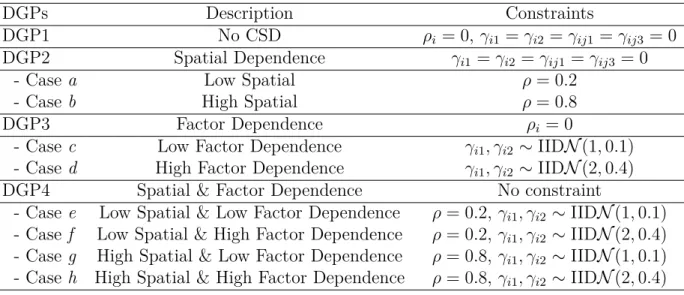
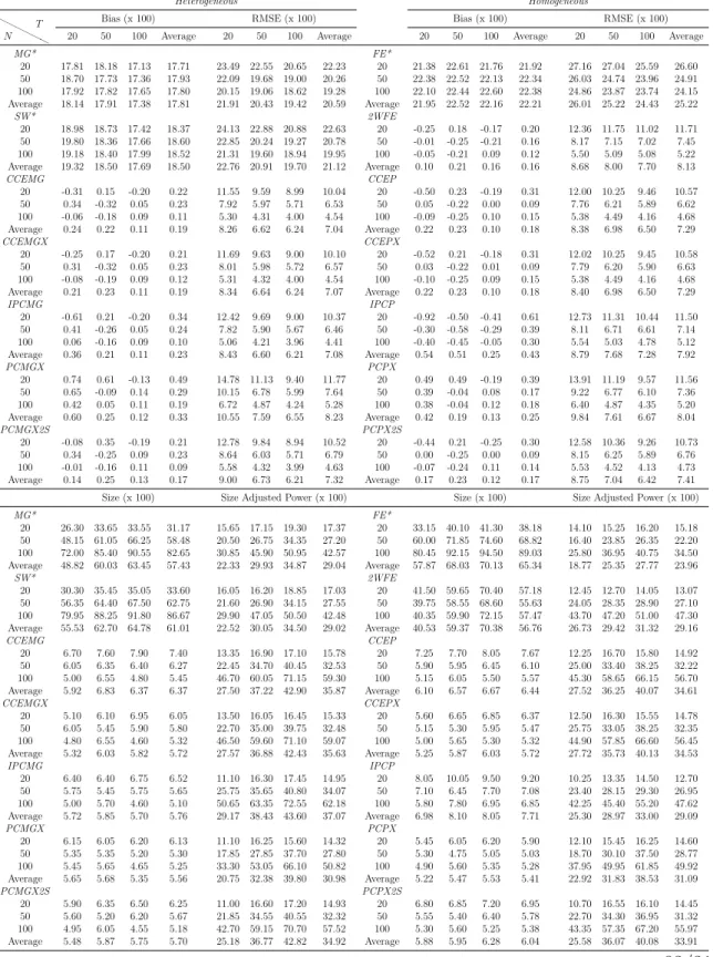
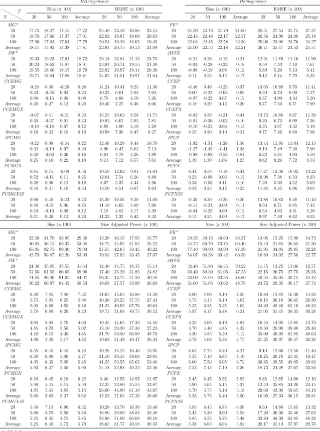
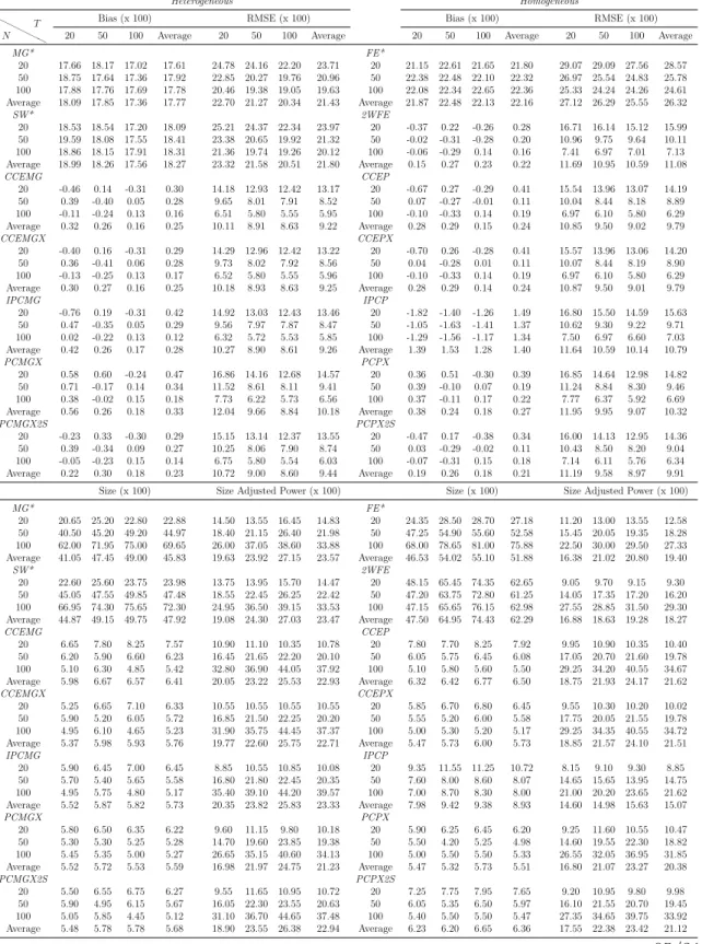
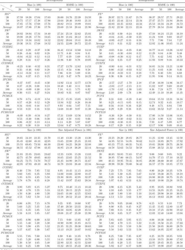
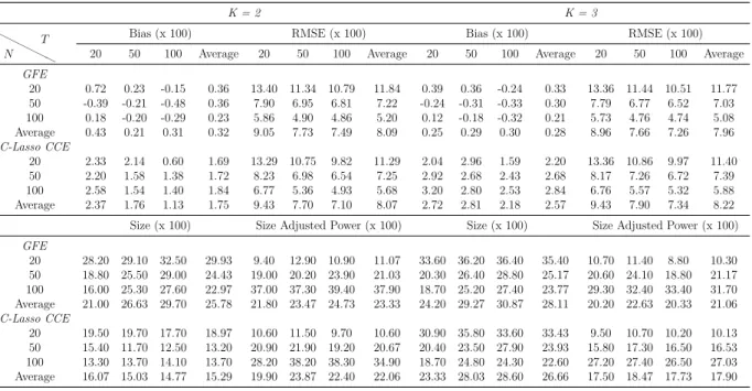
Background and Objectives: The main aim of this chapter is to investigate the impact of weak cross-sectional dependence (WCD) and strong cross-sectional dependence (SCD) on the performance of heterogeneous and homogeneous estimators in presence of low and high degrees of heterogeneity. In this chapter, a general heterogeneous panel data model which includes simultaneously unobserved common factors and spatial error dependence is presented. The associated estimation procedures are documented and a novel forecasting method for the panel data models with unobserved common factors is proposed.

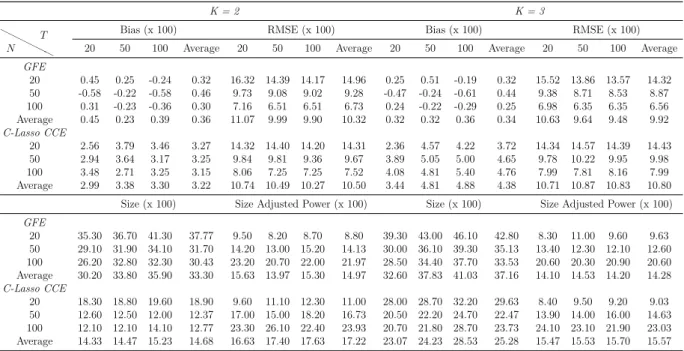
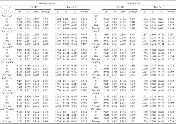
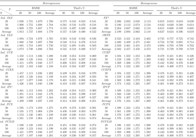
Methods: By means of simulations, the estimation, inference and forecasting perfor-mance of 16 estimators is evaluated. The estimators taken into account are mainly con-nected to the papers by Swamy (1970), Pesaran (2006), Kapetanios and Pesaran (2007), Bai (2009), Song (2013), Bonhomme and Manresa (2015) and Su et al. (2016). These es-timators comprise of heterogeneous, homogeneous and partially heterogeneous eses-timators. The performance of these estimation and forecasting procedures are compared by means of an extensive Monte Carlo exercise. The simulation framework is held in a level that is general enough to encompass recent important contributions in the panel data literature. Results and Conclusions: The main results of this chapter can be summarized as follows: (i) Even for small T and n, heterogeneous estimators, especially the mean group (MG) estimator based common correlated effects (CCE) method of Pesaran (2006) and the MG

(39)

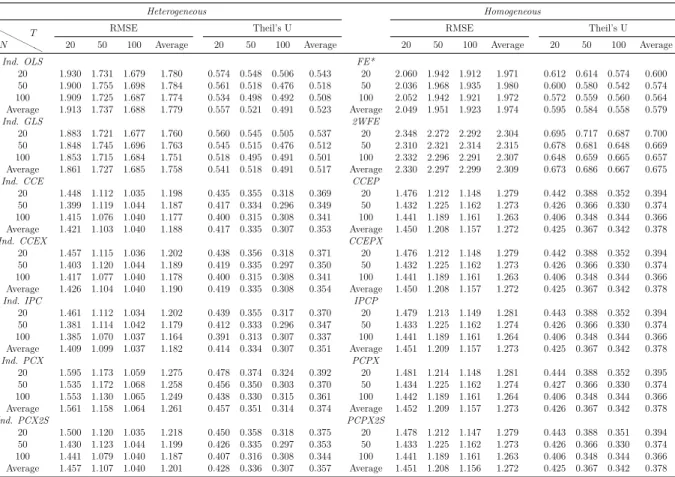
estimator based on the iterative principal components (PC) approach of Bai (2009) and Song (2013), outperform their homogeneous counterparts. However, most of the estimators considered show desirable small sample properties. (ii) The dominance of the heterogeneous estimators are more pronounced for the cases of high heterogeneity, as expected, and this main result holds for different degrees of spatial dependence and factor dependence as well. (iii) The main difference on the performance of the two methods of dealing with unobserved common factors, namely CCE and PC, occurs when we change from low to high spatial dependence; whereas changing from low to high factor dependence does not make a big difference in their comparative performance. The estimators based on PC methods are found to be more robust to spatial dependence. This result shows that both methodology work equally good against unobserved factors. (iv) Among the two estimators assuming a grouped structure of heterogeneity, the grouped fixed effects of Bonhomme and Manresa (2015) performs well in terms of bias and root mean squared error (RMSE); whereas the classifier Lasso of Su et al. (2016) based on CCE transformation gives less satisfactory results. The performance of the grouped fixed effects estimator improves as the number of groups assumed in the estimation increases. (v) The findings above are confirmed by the forecasting exercise. Namely, the forecast accuracy of heterogeneous estimators measured by mean absolute error (MAE), RMSE, Theil’s U statistic is better than their homogeneous counterparts.

Chapter 2: Equal Predictive Ability Tests for Panel Data. In the second

chapter a hypothesis testing issue is taken into consideration. The equal predictive ability (EPA) test of Diebold and Mariano (1995) is generalized to panel data sets with hetero-geneity and CD.

Background and Objectives: The main aim of this chapter is to propose tests for the EPA hypothesis for panel data taking into account both the time series and the cross-sections features of the data. Novel tests of EPA are proposed allowing to compare the predictive ability of two forecasters, based on n units, hence n pairs of time series of observed forecast errors of length T , from their forecasts on an economic variable.

Two types of tests of EPA are developed. The first one focuses on EPA on average over all panel units and over time. This test is useful and of economic importance when the researcher is not interested in the differences of predictive ability for a specific unit but

(40)

the overall differences. In the second type of tests, to deal with possible heterogeneity, the focus has been put on the null hypothesis which states that the EPA holds for each panel unit.

Methods: An exploratory analysis on the historical forecast errors of the Organisa-tion for Economic Co-operaOrganisa-tion and Development (OECD) and the InternaOrganisa-tional Mon-etary Fund (IMF) is conducted. This analysis and the previous literature suggest some stylized facts about the forecasts made by the two organizations: (i) Common Factors: the forecast errors of different countries are affected by common global shocks, (ii) Spatial Interactions: for countries which are closer to each other the comovement of the forecast errors are stronger, and (iii) Heterogeneity: international agencies make systematic errors for some particular groups of countries. The tests are developed to reflect these properties observed in the data.

To deal with WCD and SCD, the recent literature on PC analysis of large dimensional factor models (Bai and Ng, 2002; Bai, 2003) and covariance matrix estimation methods which are robust to spatial dependence (Kelejian and Prucha, 2007) have been followed.

The small sample properties of the tests proposed are investigated via an extensive Monte Carlo simulation exercise. In a time series framework the small sample properties of heteroskedasticity and autocorrelation consistent (HAC) estimators are well-known and comparison of the role of different kernel functions in the estimation performance is readily available (see Andrews, 1991). Whereas, in spatial modeling the Monte Carlo analysis on spatial heteroskedasticity and autocorrelation consistent (SHAC) estimators is limited to only the work of Kelejian and Prucha (2007). In this chapter, their analysis is extended in several dimensions, such that we consider many different combinations of time and cross-sectional dimension sizes and allow for several different kernel functions to investigate their role on small sample properties of the EPA tests.

Results and Conclusions: The small sample properties of the proposed tests have been found to be satisfactory in a large set of Monte Carlo simulations. In particular, the tests which are robust to SCD are found to be correctly sized in all experiments. This is the case even in the experiments which do not involve common factors but only spatial dependence. However, their power is generally low compared to test statistics which are robust only to spatial dependence, given that forecast errors do not contain common factors. In these

(41)

cases, the Monte Carlo evidence suggests to use Bartlett and Parzen kernels for correctly sized test.

In the empirical application, it is found that IMF has an overall better performance in terms of bias whereas OECD makes predictions with less variance. However, the differences are rarely statistically significant. In a sub-sample of G7 countries OECD predictions are found to be superior to that of IMF.

Chapter 3: Multistep Forecasts with Factor-Augmented Panel Regressions.

The third chapter goes further in the analysis on panel data forecasting. It contains an extensive empirical comparison of several models and methods of panel data in terms of their forecasting ability.

Background and Objectives: In this chapter, the optimal forecasting strategies using a general dynamic heterogeneous panel predictive regression model is explored. The model under consideration allows predicting unit specific outcomes with global common factors in macroeconomic variables. The main aim is to propose and compare forecast methods using such panels with unobserved common factors. Empirical iterated and direct forecasts are compared using two different forecasting approaches developed for panels with common factors. The first one uses estimates of the common factors in the predictive model by applying principal components analysis (PCA) on the residuals from a first stage consistent estimation of the slope coefficients. The unobserved nature of the common factors requires forecasting the future values of these estimated factors first, then computing the predictions on the variable of interest in a following step. In the second approach, the common factors are estimated from a number of auxiliary variables as in the works of Stock and Watson (2002a) and Bai and Ng (2006). The difference between these studies and used in this chapter is that here, common factors are estimated from the realizations of the same variable for different panel units whereas in their studies these factors come from a large number of indicators for the same panel unit. Although, the approach does not rule out the possibility of having several variables correlated with the common factors.

Methods: This chapter uses empirical forecasts to compare the properties of different methods and estimators. For this purpose, the data set is divided into an estimation and a prediction period. Mainly, the out-of-sample forecasting methodology of Marcellino et al. (2006) is followed. Two different accuracy measures are used: the RMSE and the MAE.

(42)

The comparison is done by comparing the distribution of these statistics over countries in the sample.

Results and Conclusions: The results showed that the direct method outperforms the iterated strategy in almost all cases. Comparison of the models with and without global common factors showed a clear dominance of the methods using global information in forecasting country specific variables. Finally, heterogeneous estimators of the slope pa-rameters are found to outperform the homogeneous estimators in simple models. For large and more complex models, pooling has advantages for forecasting purposes.

(43)

Chapter 1 Heterogeneity and Cross-Sectional

Dependence in Panels

1

In this chapter, we focus on the comparison of heterogeneous and homogeneous panel data estimators in presence of cross-sectional dependence modeled by spatial error dependence, common factors or both. These specifications allow us to consider weak cross-sectional dependence (connected to a spatial weight matrix) and strong cross-sectional dependence (common factors). The estimation procedures are described and a forecasting approach is proposed in the presence of unobservable common factors. An extensive Monte Carlo study is conducted using a general framework able to encompass recent seminal contributions in the literature. The results show that even for small individual and time dimensions heterogeneous estimators perform better in terms of bias, RMSE, size and size adjusted power of two-sided tests. Statistical accuracy measures also confirm that the best forecasts are associated to heterogeneous estimators.

1_{This chapter is based on two papers written with Alain Pirotte and Giovanni Urga submitted to Revue}