Mechanical Analysis of Doxorubicin Induced Cardiotoxicity on an Animal Model

(1)

affiliée à l’Université de Montréal

Mechanical Analysis of Doxorubicin Induced

Cardiotoxicity on an Animal Model

ERIC BUZAGLO Institut de génie biomédical

Mémoire présenté en vue de l’obtention du diplôme de maîtrise ès sciences appliquées Génie biomédical

Juin 2019

(2)

POLYTECHNIQUE MONTRÉAL

affiliée à l’Université de Montréal

Ce mémoire intitulé :

Mechanical Analysis of Doxorubicin Induced

Cardiotoxicity on an Animal Model

présenté par Eric BUZAGLO

en vue de l’obtention du diplôme de Maîtrise ès sciences appliquées a été dûment accepté par le jury d’examen constitué de :

L’Hocine YAHIA, président

Delphine PÉRIÉ-CURNIER, membre et directrice de recherche Boris CHAYER, membre

(3)

DEDICATION

To the people who were involved with this research and for those who are directly affected by cardiotoxic anti-cancer treatments that may one day benefit.

(4)

ACKNOWLEDGEMENTS

I would like to first and foremost thank my research director Dr. Périe-Curnier for taking me under her wing for this extended study. By providing me the tools, background notions and resources, I was able to further my knowledge in the Biomedical Engineering sector, all while enriching my prior background in Mechanical Engineering. Since the very beginning, Dr. Périe-Curnier challenged me and allowed me to satiate my deep curiosity of the how and why things work in the biomedical world. A big thank you goes out as well to Boris Chayer, Lab Engineer at the CrCHUM, who patiently sat with us long hours to obtain data results for each sample we’ve tested. He also made us think more critically and helped us explore why certain graphs obtained out of order results. Another thank you is extended to Sophie Lerouge who allowed us to book the rheology room with very little trouble and giving us access to all her lab equipment. Lastly, I would like to thank Yassin Seddik and Benoit Waeckel for their involvement with this project during their stage to help accelerate what was a long list of work needed to complete my research. They’ve contributed immensely to the success of this experimentation and proved to be valuable when it came time to establishing testing protocols.

(5)

RÉSUMÉ

Objectif : La chimiothérapie a fait ses preuves au fils des années comme traitement principal permettant de détruire les cellules cancéreuses présentes dans plusieurs types de cancers. La doxorubicine a longtemps été utilisée comme un agent anti-cancérigène dans la chimiothérapie mais elle entraine des effets secondaires dans le corps tels que la suppression de plaquettes et de globules blancs, le développement de l’alopécie, ou encore la perte de myofibrille dans les parois du cœur. De plus, la doxorubicine peut amener des effets cardiaques comme un arrêt du cœur.

L’objectif de ce travail est de proposer des solutions pour détecter les effets cardiotoxiques de cet agent, au moyen de la spectrométrie Raman et de la rhéologie, en faisant des tests moléculaires et mécaniques sur des cœurs de porc.

Matériel et méthodes : Des échantillons de cœur de porc ont été récupérés d’une étude dans laquelle cinq miniporcs Yucatan femelles ont reçu une dose totale de 375mg/m2 de doxorubicine administrée en cinq fois à trois semaines d’intervalles, formant le groupe expérimental appelé groupe ‘DOXO’. Par ailleurs, deux miniporcs ont reçu une injection saline selon le même protocole, formant le groupe ‘untreated’. À l’aide d’un rhéomètre, des tests de frequency sweep et de relaxation ont été effectués sur ces échantillons pour mesurer la contrainte de cisaillement (G), le module de perte (G’’) et finalement le module de stockage (G’). En parallèle, des tests en spectroscopie Raman ont été effectués pour déterminer la composition moléculaire des échantillons.

Résultats: Nous avons obtenu un comportement linéaire pour une déformation de  =1,6% lors des tests de strain sweep. Cette déformation a été appliquée pour les tests de frequency sweep et de

(6)

contrainte-relaxation. Le test de frequency sweep nous permet de conclure à une baisse globale des propriétés mécaniques des échantillons DOXO dans le septum par rapport au groupe « untreated » alors que nous avons constaté une augmentation dans les ventricules gauches et droits. Lors des tests de relaxation, nous avons trouvé une grande diminution dans les propriétés mécaniques des échantillons du groupe DOXO par rapport au groupe ‘untreated’. Quant aux résultats de la spectrométrie Raman, nous avons obtenu une baisse générale du collagène et des lipides dans les échantillons DOXO, ce qui suggère une diminution dans la rigidité structurelle. Les résultats obtenus par rhéométrie ont été comparés aux résultats obtenus par spectroscopie Raman et nous avons observé une corrélation significative.

Conclusion: Les propriétés mécaniques et la composition chimique du tissu cardiaque ont été altérées par le traitement à la doxorubicine chez des mini-porcs Yucatan. Cette experimentation, associée à de futures études, permettra de définir de nouveaux biomarqueurs des traitements à la doxorubicine, et à long terme de trouver des solutions permettant de réduire l’effet cardiotoxique.

Mots clés: Cardiotoxicité, Doxorubicine, rhéométrie, Strain Sweep, Frequency Sweep, Test de contrainte-relaxation, Spectrométrie Raman

(7)

ABSTRACT

Purpose: Chemotherapy has been proven to be the best way to eliminate several types of cancer. However, derived from this form of treatment is its cardiotoxic damage and overall functioning of the human heart. Young patients receiving a high dosage are the most prone to develop this cardiotoxicity, which can occur either early or late after treatment. This study aims to specifically investigate the effects doxorubicin has on the overall mechanical and morphological properties in the heart.

Material & Methods: Five young female miniature swines received five 75mg/m2_{injections of} doxorubicin every three weeks for a total cumulative dose of 375mg/m2, constituting the experimental group called DOXO samples. Two miniature swines received a saline injection under the same protocol, constituting the untreated group. These samples were subjected thereafter to frequency sweep and stress-relaxation test in order to determine the shear modulus (G), loss modulus (G”) and storage modulus (G’) using a rheometer. In parallel, samples were also placed in a raman probe after being submerged in a saline solution. This was used for the Raman Spectrometry portion of the experimentation where the goal of this last one was to determine to molecular composition of each sample tested through the notions of detecting various Raman shift along the domain.

Results: Miniature swines receiving chemotherapy yielded a difference in the mechanical properties. The septum portion of the heart showed an overall diminishment in the storage and loss modulus whereas the left and right ventricle showed an overall strengthening of these parameters. The stress-relaxation test which is the most deterministic test studied showed a clearer drop in the mechanical properties of the DOXO samples. In the Raman Spectrometry study, results obtained

(8)

showed an overall decrease in the collagen and lipids content in the DOXO samples. This can be linked potentially to the overall degradation of the sample’s structural rigidity. This is why there was a strong correlation between the mechanical testing conducted and the Raman Spectrometry test.

Conclusion: The mechanical properties and the chemical composition of the cardiac tissue altered but the doxorubicin treatment on the Yucatan miniature swine. The combination between this experimentation and future advancements will help characterize biomarkers for the doxorubicin agent, which can ultimately lead to finding solutions on how to reduce its manifestation on the central cardiac cavity.

Keywords: Cardiotoxicity, Doxorubicin, Miniature Swine, Rheometry, Strain Sweep, Frequency Sweep, Stress-Relaxation Test, Raman Spectrometry

(9)

LIST OF TABLES

Table 3.1 Three sub-solutions needed to compose the Tyrode Solution ... 25

Table 3.2 Ratio needed for the mixture of the three sub-solutions ... 25

Table 3.3 Samples retrieved from Yucatan parts ... 28

Table 4.1 Raman table for Raman Shift equal to 602cm-1 ... 77

Table 4.2 Table identifying the various molecules found given the Raman shift ... 79

Table 4.3 Raman Shift and P-values for the Septum ... 80

Table 4.4 Raman Shift and P-Value for the Right Ventricle ... 81

Table 4.5 Raman Shift and P-value for the left ventricle samples ... 82

(12)

LIST OF FIGURES

Figure 2.1 Anatomy of heart……… 4

Figure 2.2 Blood Circulation……… 5

Figure 2.3 Layer Composition of the Heart Wall………. 6

Figure 2.4 Anatomic structure comparing the main types of Anthracycline………... 8

Figure 2.5 Two-plates model used to define the shear stress using the parameters shear force F and shear area A of the upper, movable plate………... 14

Figure 2.6 Torsion Flow in Parallel Plates………. 14

Figure 2.7 Selection of Spindle based on Sample Diameter……….. 15

Figure 2.8 Plate Gaps Relative to the Shear Rate………... 16

Figure 2.9 Plate Diameter Relationship to the Shear Stress………... 16

Figure 2.10 Components of the Antor Paar MCR 301 Rheometer……… 17

Figure 2.11 Scattering of Light by Molecules……… 19

Figure 2.12 Diagram of the Rayleigh and Raman Scattering Processes………….……….. 20

Figure 2.13 Raman spectrum of Ethanol……… 21

Figure 2.14 Determining the level of crystallinity by analyzing the Raman peak………. 21

Figure 3.1 Parts before the requisition of samples used for experimentation……… 23

Figure 3.2 Samples being prepared before being placed in the Rheometer………... 23

Figure 3.3 Preparation of the three sub-solutions at the CEPSUM……… 24

Figure 3.4 Holder for Peripheral Cut……….. 26

Figure 3.5 Slicer………. 26

Figure 3.6 Sample being placed under the rheometer’s spindle………. 30

(13)

Figure 3.8 Pythagorian relationship between shear modulus, storage modulus and loss modulus 33

Figure 3.9 Results of the Strain Sweep from 1Hz to 100Hz for butcher samples……….. 36

Figure 3.10 Linearity test finding R2 for the Strain Sweep [1.7-1.9] %... 37

Figure 3.11 Linearity test finding R2 for the Strain Sweep [1.5-1.7%]………. 38

Figure 3.12 Storage Modulus Test Results Butcher Samples……… 39

Figure 3.13 Complex Viscosity Frequency Sweep Test on Butcher Samples………... 40

Figure 3.14 Loss Modulus Frequency Sweep Test on Butcher Samples………... 40

Figure 3.15 Visual Relationship between Complex Viscosity, G’ and G’’………... 41

Figure 3.16 Storage Modulus Comparing Butcher to Untreated Samples………. 42

Figure 3.17 Average Storage Modulus results for the Left Ventricle Samples………. 43

Figure 3.18 Average Complex Viscosity for Left Ventricle Samples………44

Figure 3.19 Average loss modulus for Left Ventricle Samples………. 45

Figure 3.20 Average Storage Modulus Frequency Sweep Septum……… 46

Figure 3.21 Average Complex Viscosity Frequency Sweep Septum……….47

Figure 3.22 Average Loss Modulus Frequency Sweep Septum……….48

Figure 3.23 Frequency Sweep results for right ventricle………49

Figure 3.24 Relaxation Test Posterior Left Ventricle……….50

Figure 3.25 Average Relaxation Test Left Ventricle………. 51

Figure 3.26 Average Relaxation Test Septum……… 52

Figure 3.27 Fractured Septum Sample 98……….. 53

Figure 3.28 Frequency Sweep redone post relaxation test on left ventricle samples………. 54

Figure 3.29 Frequency Sweep redone on septum samples post relaxation test………. 56

Figure 3.30 Frequency Sweep redone on right ventricle samples post relaxation test………….. 57

(14)

Figure 4.1 Raman Probe used for experimentation……… 72 Figure 4.2 Raman Curve Posterior Left Ventricle DOXO………. 74 Figure 4.3 Raman Spectrometry data superposing both DOXO and untreated samples………… 75 Figure 4.4 Difference in Raman shift peak……… 76

(15)

LIST OF SYMBOLS AND ABBREVIATIONS

ACIA Agence Canadienne d’inspection des aliments

ANT Anterior

CEPSUM Centre d’éducation physique et des sports de l’Université de Montréal CIPA Comité Institutionnel de Protection des Animaux

CMR Cardiovascular Magnetic Resonance

CrCHUM Centre de recherché Centre Hospitalier Université de Montréal

G Shear Modulus

G’ Storage Modulus

G” Loss Modulus

LV Left Ventricle

MFD Mean Fiber Direction

MRE Magnetic Resonance Elastography

MRI Magnetic Resonance Imaging

POST Posterior

(16)

LIST OF APPENDICES

Appendix A – Graph Generation Sample Codes ... 103 Appendix B – Table Generation Frequency Sweep For Each Sample Code ... 112

(17)

CHAPTER 1 INTRODUCTION

The doxorubicin agent, a form of anthracycline, used for many years as an anti-cancer agent during chemotherapy, has reliably helped patients on their road to remission. However, this agent has also been linked to cause cardiotoxic affects in the heart such as the suppression of platelets and white blood cells, the development of alopecia, causing hair loss, and morphological effects such as the loss of myofibrils on the walls of the heart (Aissiou et al., 2016). More notably, doxorubicin can have permanent effects such as a degradation of the heart’s function. The two most commonly used anthracyclines up until now has been doxorubicin and epirubicin (Kaklamani et al., 2003).

There has been attention drawn to patient’s heart condition post chemotherapy and the long term impact anthracyclines has on the heart. Making use of echocardiography and MRI, studies were conducted to understand the long-term impacts the treatment poses on the heart though it has been difficult to draw conclusions on the effectiveness these imaging tools have on not only detecting the associated cardiotoxicity but characterizing it as well. This raises the need to further explore the fundamental understandings of the evolution of this cardiotoxicity, characterizing it by finding biomarkers, and to ultimately find methodologies to reduce its cardiotoxic effects, all in the intention to benefit the recipients receiving these treatments.

Though the digestive system presents anatomical differences between a swine’s heart with that of a human, the miniature swine heart’s structure, function and anatomy make this animal a good overall candidate for this research (Kohn et al., 2011). In addition, the miniature swine’s heart

(18)

presents similarities in the form of heart damages and side effects to humans where the treatment regimen is similar to those used in a clinical setting (Herman and Ferrans, 1983). These reasons highlight why the miniature swine is of particular interest for the study of doxorubicin. Adopting the miniature swine as a model based on the previous mentions allows us to formulate the following scientific objective:

O1- Characterize the mechanical properties of the myocardium following doxorubicin chemotherapy on animal samples.

O2- Characterize the chemical properties of the myocardium following doxorubicin chemotherapy on animal samples.

O3- Characterize the doxorubicin cardiotoxicity from the combination of mechanical and chemical parameters of the myocardium.

The hypothesis of this research is that samples from animals exposed to doxorubicin will have diminished mechanical properties when withstanding the torsional and shear stresses applied on both sets of samples. The hypothesis will be refuted if the mechanical properties remain similar when comparing doxorubicin-induced samples versus non-treated samples.

In the second chapter, a critical literature review will be presented to help define the different notions allowing to deepen the reader’s understanding behind the context of the research at hand. Following this, the third chapter will go over the experiments and protocol put in place to conduct the tests along with the results obtained. The fourth chapter will also go over the secondary form of experimentation on our samples which involve Raman Spectrometry. Lastly, the perspectives drawn from these studies will allow for further future advancements.

(19)

CHAPTER 2 LITERATURE REVIEW

Heart Anatomy

The heart’s function is to circulate oxygenated and deoxygenated blood throughout the body including its extremities. It is composed of muscular fibers and is considered to be the primary motor organ of the human body. The functioning of the cardiac cycle is explained from the contraction of four of its main chambers which includes the left atrium (LA), the right atrium (RA), the left ventricle (LV) and the right ventricle (RV). These last two are subsets of the apex and can be located near the bottom as conveyed in (Figure 2.1). The interatrial septum is what separates the two atrium cavities while the interventricular septum is what separates the lower left and right ventricules. This separation causes the inability for both the atriums and the ventricles to not being able to communicate to one another. However, the right ventricle can communicate to the right atrium via the tricuspid valve. On the opposite side, the mitral valve is what helps connect the left ventricle from the mitral valve.

(20)

Three major components that culminate the cardiac system are the blood vessels, the blood vessels themselves and finally, the heart. In order to oxygenate the blood, at every contraction, blood is pumped towards the inside of the cavities and is then circulated towards all the remaining organs in the body. We refer ourselves to the schematic, which describes the transfer from deoxygenated to oxygenated blood (Figure 2.2). The two circuits of the cardiac function are the pulmonary circulation and the systemic circulation. Firstly, the pulmonary circulation consists of deoxygenated blood entering the right ventricle through the lungs where it is then sent to the left Figure 2.1- Anatomy of heart – modified from Human physiology – The Mechanisms of Body Function (Widmaier, 2014)

(21)

atrium. When blood is oxygenated during the pulmonary circulation, the blood returns to the left atrium via the pulmonary veins, sent to the left ventricle where it is then distributed throughout the major organs with the help of the aortic valve. The blood is then sent through the systemic circulation from the left ventricle, going through all the tissues and organs found around the body where it is then deposited in the right atrium. In both circuits, the vessels carrying blood away from the heart are known as the arteries. The vessels where blood is incoming are better known as veins.

Figure 2.2 Blood Circulation – modified from https://www.pdhpe.net/the-body-in-motion/

The systole and diastole are the two main phases that represent the cardiac cycle. The systole phase takes place when the heart contracts to pump blood out by contracting itself. On opposite ends, the diastole relaxes the heart after its contraction and fills out the two atrium chambers with blood.

(22)

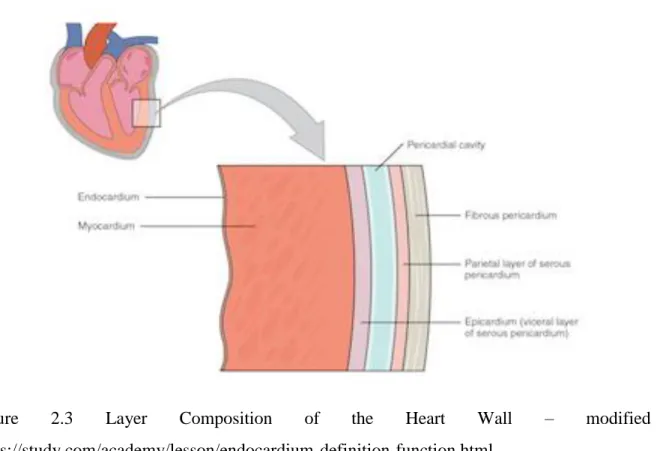
The cardiac tissue that encapsulates the cavity is composed of three distinctive layers; each with their distinctive role and property. These thin sheets superposed one on top of the other allow for an easier systole and diastole phase to take place during the cardiac cycle. The primary layer which constitutes as the main layer of the cardiac tissues is called the myocardium, also known as the muscular tissue of the heart. This layer comprises the majority of the heart’s weight and is sandwiched between the two inner and outer layer. Within this layer lay the cardiomyocyte cells whose role is to carry information to the nervous system allowing the nervous system to send a signal to trigger the heart’s contraction or relaxation. The inner most layer is called the endocardium tissue which is a smooth membrane covering the inner chambers of the heart. The outer most layer is the epicardium layer which is considered to be the skeletal layer of the cardiac tissue.

Figure 2.3 Layer Composition of the Heart Wall – modified from

(23)

The outer most layer also known as the extracellular matrix, collagen can be found and provides support to the tissues encapsulating the heart. This fiber, which is most frequently, allows the cardiac muscle to not only maintain its global shape but permits it to be either flexible or resistant during the cardiac cycle. Other important fibers include the elastine which allows for a greater elasticity of the myocardium space. This elasticity is important in order to prevent tears. Most studies covering the extracellular matrix of the myocardium’s mechanical function base themselves on the different types of fibers found and play an important overall role to the extracellular matrix.

Forms of Cancer Treatments and its effects

Anthracycline chemotherapy is still to this date an important form of treatment to eliminate cancer cells. This administered potent drug is a class of chemotherapeutic agent extracted from Streptomyces bacterium. The beneficial effects from anthracycline span from hematological malignancies to solid tumors (Moudgil et al., 2017). Anthracyclines interferes with the cancer cell’s DNA metabolism and the production of its RNA once it is injected. By inducing the patient with oxygen-derived free radicals and superoxides through the injection of anthracycline, this causes damage to the cell’s DNA by inhibiting a synthesis from further taking place causing them to die. There are four types of very similar anthracyclines; daunorubicin, doxorubicin, idarubicine and epirubicin. The first molecule explored in the early 1960s when anthracycline chemotherapy

(24)

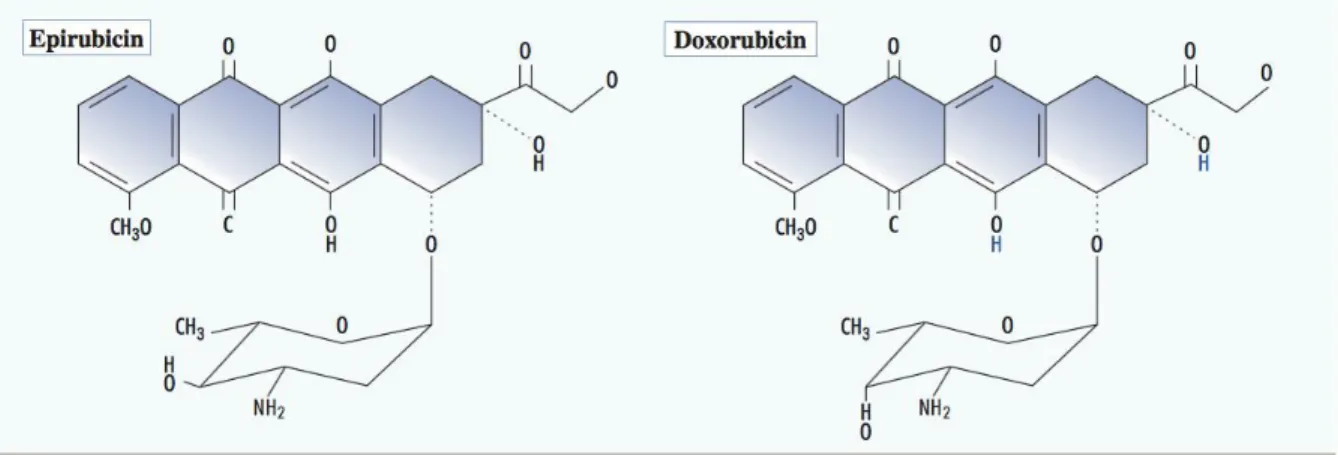
was explored was the daunorubicin drug (Butler et al., 2009). This red potent liquid prevented cancer cells to split into two due to tangled DNA strands which help slow down or eliminate cancer cell growth. Since then, doxorubicin has emerged as being the most widely used anthracycline though there still advantage in using the 3 other anthracyclines in certain cases such as daunorubicin for the treatment of acute leukemias (Kaklamami et al., 2003). Doxorubicin’s use in breast cancer started after the observation that it produced high response rates in metastatic disease. Metastatic disease is the medical term used for cancer that spreads from one original place in the body to another. Since this discovery, numerous tests to treat early-stage breast cancer have allowed doxorubicin to be a core component of chemotherapeutic regimens (Kaklamami et al., 2003). Epirubicin, the 4'-epimer of doxorubicin (Figure 2.4) is also highly active in treating metastatic disease and was created because of its proven clinical testing to prevent a higher toxicity profile than that of doxorubicin. Epirubicin differentiates itself structurally from doxorubicin in the epimerization of the hydroxyl group in position 4 of the amino sugar moiety (Kaklamami et al., 2003). Both drugs are metabolized in the liver and eliminated through the bile (Zhang et al., 2014).

Figure 2.4 Anatomic structure comparing the main types of Anthracycline – modified from (Kaklamami et al., 2003).

(25)

Side effects of anthracycline are numerous such as the suppression of platelets and white blood cells in the bone marrow, diarrhea, but mostly alopecia, which causes human hair loss and other morphological effects such as the loss of myofibril on the outer shell of the heart. Most notably, the main and serious side effects of anthracycline during cancer chemotherapy is its cardiotoxic impact, which remains the main focus of this research.

Anthracycline administered into the human body in intravenous form can be subdivided into three stages of cardiotoxic effects. At the first stage, the effects are already evident after a single administration, which includes disturbances in cardiac rhythm and changes in blood pressure (Pecoraro et al., 2017). The second stage includes cardiac dilation and cardiomyopathy, a disease in the heart’s muscle. Lastly, the third stage of cardiotoxic effects due to anthracycline is terminal due to a stop of the heart’s function (Pecoraro et al., 2017). Doxorubicin-induced cardiotoxicity is mainly related to the accumulation of the repetitive doses required during a patient’s treatment process. The dose administered varies from patient to patient but is usually between 30 and 70mg/m2_{with a maximum cumulative administration of 120 mg/m}2 _{(Schellens et al., 2005). The} accumulation of these doses cannot exceed 500 mg/m2 _{which implies a maximum treatment period} of four weeks though recent studies indicate damages caused by anthracycline are noticed even after a single administration (Pecoraro et al., 2017).

(26)

The exact cause of anthracycline’s cardiotoxic effects is not fully explored nor understood but it is assumed to be due to a multitude of reasons. Several studies indicate that doxorubicin induced cardiomyopathy is characterized by abnormal calcium homeostatis (Zhang et al., 2014). Doxorubicin administration is able to induce calcium dysregulation and Connexin43 (Cx43) in a rat’s cardiomyoblast cell line noticed immediately after administration (Pecoraro et al., 2015). The aim of this study was to investigate the effects of DOXO administration on Cx43 expression and localization in a short-term model where they performed an echocardiography on mice.

In order to reduce the cardiotoxic effects, researchers have analyzed many options over the course of the past decades. A published study by Geisberg et al. highlights a few strategies considered to help reduce or eliminate anthracycline’s cardiotoxicity (Geisberg et al., 2010). The first includes limiting the cumulative exposure of anthracyclines. This would entail encapsulating anthracyclines in liposomal microparticles or modifying the rate of discussion (Geisberg et al., 2010). Encapsulating the drug seems to have been a preference in the study because of “vascular permeability changes in malignant tissue.” Other strategies included changing the rate of anthracycline’s administration, making changes to the formulation or also exploring alternative drugs that present less of cardiotoxic effect. In another study covered by Conway et al. he proposed similar tactics to minimize the cardiotoxic impact. There is alternative medication called dexrazoxane, which mimics the behavior of anthracycline. However, dexrazoxane has a negative

(27)

impact on the bone marrow’s function due to the increase of myelosupression (Seymour., et al 1999). Next, avoiding the administration all together is something to be considered though the original purpose of anthracycline is to help kill the DNA in the cancer cells. Another study conducted by Dalen et al. proposes other agents as a substitute such as iron chelator, dexrazoxane as a means to reduce anthracycline-induced free radical formation (Dalen et al., 2005). While trying to prevent the cardiotoxic effect, Dalen et al. mentions potential adverse effects including limits to the tumor response (Dalen et al., 2005). However, the study concludes a more favorable outcome this drug has on the cardiotoxic impact.

All these techniques presented in all three articles can potentially help reduce or eliminate anthraycline’s cardiotoxic effects. Unfortunately, the combined studies up until now still do not provide a sufficient amount of biomarkers that would ultimately help draw concrete solutions on the cardiotoxity levels of the doxorubicin agent. This is where the added value of this research report comes in so that drawing conclusions from the characterization of doxorubicin’s cardiotoxicity based on the mechanical test results can help determine methods such as effective injection concentrations of doxorubicin, clinical diagnostics, therapeutic interventions or material design for tissue engineering.

Animal studies of Anthracyclines Cardiotoxic Effects

The study regarding the cardiotoxic effects of doxorubicin originated with Mettler et al. where he made use of a rat model. The evaluation and the feasibility of the rat as a pertinent model was demonstrated in this study (Mettler et al., 1977). This study found that the overall mass of the rats treated with doxorubicin had dropped compared to the untreated models (Robert et al., 2007). Since then, newer adapted protocols, which includes variations in the anthracycline dosages and

(28)

concentration, were introduced. Another study using non-rodent animals such as guinea pigs, rabbits, dogs and non-human primates received seven dosages (1mg/kg) of doxorubicin during the span of 7 weeks. The subjects were unable to gain any weight during the experimentation in addition to suffering from respiratory problems linked to the interrupted cardiac cycle (Vargas et al., 2015).

Another study conducted by Herman et al. in the early 80s provided weekly dosages of 1mg/kg over the course of four months to dogs (Swindle et al., 2012). After four months of close monitoring, the results showed a loss of myofibril protein in the doxorubicin treated subjects. Like the previous studies, the dogs were subjected to weight loss over the course of the study (Swindle et al., 2012).

Although many animal models have been used to study doxorubicin toxicity, several restrictions limit their use. This is why Manno et al. chose a non-rodent animal, specifically the guinea pig as a mean to further study anthracycline’s impact on the myocardium. In total, three groups of three female and male miniature swines received 1.5mg/kg at intervals of three weeks over seven cycles. A weight loss was observed in the female model after only four cycles while there were suppression effects of doxorubicin on the bone marrow which caused hematological suppression on all 18 subjects. Such effects caused a decline in the red blood cells. The study concludes by stating that due to the close resemblance of the minipig to the human heart, this model should be the non-rodent species of choice for all future testing involving the study of doxorubicin (Manno et al., 2015).

In 2013, Dr. Curnier experimented with Doxorubicin induced models and referred the study of myocardial damage using endomyocardial biopsy of the right ventricle to be the “gold standard”

(29)

(Mohamed et al., 2013). It provides reliability however poses disadvantages such as it being an invasive procedure which can cause risks so necessary training is needed in order to study the symptoms of doxorubicin using this approach. Concerning the left ventricle, 2D and 3D echocardiography has proven through this study to properly estimate the ejection fraction and information such as area and volume measurements. The results obtained showed to have similar results to that of cardiovascular MRI (Mohamed et al., 2013).

Up until now, many studies conducted on the myocardium model involved histological analysis, MRI testing and imaging protocol such as cardiovascular MR (CMR) but very little development has emerged on the actual mechanical properties of the samples. The study, which compares the mechanical properties of the untreated and treated samples, will allow the characterization of structural damages induced on the heart from a mechanical standpoint. A device formally used to study tissue properties is the rheometer and will be discussed in the following literature review, which covers the science of rheology.

Characterization of tissues mechanical behavior using Rheological Testing

Rheology is a technique to measure and describe the overall behavior and deformation of any form of solid material. A popular equipment that measures all forms of deformations such as the shear stress of a material is the rheometer. The rheometer measures with high precision information such as the rotation and step strain using a sample-adaptive controller, the gap measurement and thickness of samples and the normal force of a material using high-precision air bearings. There are two types of rheometer. The first is a rheometer that controls the applied shear stress or shear strain better known as the shear rheometer. The second is called an extensional rheometer, which,

(30)

as the name describes, applies an extensional stress, or extensional strain on samples being studied (Pipe, Majmudar and McKinley et al., 2008).

An important measurement used for this experimentation is the shear stress which can be defined as:

τ = F / A

where F is the shear force (in N, newton) and A is the shear area A (in m2_{). The unit for shear stress} is 1 N/m 2 = 1 Pa (Pascal). A rheometer records the shear force via the torque at each measuring point.

The two-plate model is used to define the rheological parameters to better understand matter’s behavior. For example, shear is applied to a sample sandwiched between two plates. The lower plate (base) is mounted on a very rigid support and the upper plate can be moved parallel to the lower plate which in the rheometer’s case is the spindle as seen in Figure 2.6.

Figure 2.5 Two-plates model used to define the shear stress using the parameters shear force F and shear area A of the upper, movable plate – modified from https://wiki.anton-paar.com/en/basics-of-rheology/

(31)

The shear stress can also be defined as the relationship between the spindle’s radius and the torque

seen in Figure 2.6.

 =

𝟐

𝝅𝒓𝟑

x M

where  = shear stress

r = plate radius M = torque in N . m

The shear strain is defined as the relationship between the plate’s spacing, angular motor deflection

and the plate radius.

 =

𝒓

𝒉

x 

where  = shear strain r = plate radius

h =distance between 2 plates

 = angular motor deflection in radians

It is important when it comes to selecting the spindle dimension to choose one that will correspond not only to the specimen dimension but to its viscosity as well. A low viscous substance such as milk should be measured with a spindle diameter equal to 60mm, a medium viscous substance such as honey should be measured with a spindle diameter equal to 40mm and a highly viscous substance such caramel or tissue culture should be measured with a spindle diameter of either 20mm or 25mm (Kalyanamaran et al., 2012).

(32)

The greater the spindle’s circumference, the better suited it is to analyze smaller changes in sample’s deformation and is more optimized for increased sensitivity. In addition, the smaller the shear stress that is applied on the substance located in between the plates. This holds true by

analyzing the mathematical equation defining the shear stress:

 =

𝟐

𝝅𝒓𝟑

x M

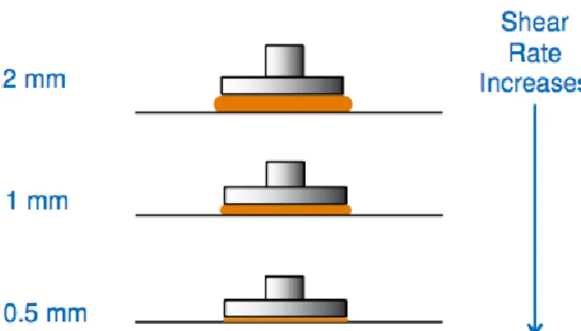
Another important component of calculating substance properties is by measuring the thickness of the material being placed in between the plates. As the gap height between the plate decreases, the overall shear rate applied to the material increases.

Figure 2.8 Plate Diameter Relationship to the Shear Stress

(33)

The shear rate can be defined as the following: 𝛾̇ = x𝑟 ℎ where γ̇ = shear rate

 = Motor angular velocity in rad/sec

r = spindle radius

h = distance between 2 plates

The specific rheometer used for the experimentation at the CrCHUM, Centre de recherché Centre Hospitalier Université de Montréal, was the MCR 301 fabricated by Antor-Paar, which can be found in Figure 2.10. The advantage of a two-plate rheometer is the ability to perform long stress-relaxation tests for a multitude of substance shape size and viscosity.

In a rheometer, the loading applied on a material and the stress is derived from the torque. The formula for stress is

where

(34)

and the stress constant, , is a geometry dependent factor.

Aside from characterizing biomarkers using mechanical testing with the aid of the rheometer, the goal of the experimentation is to link these results with those of the results obtained in Raman spectrometry.

Raman Spectrometry

Spectrometry is a science technique used in chemistry to help identify molecules based on the observed vibrational, rotational and other low frequency modes in a given system. This technique

uses a laser light source at frequency 𝜔0 to irradiate a sample in order to generate Raman scattered light. The Raman spectrum allows then to identify the fingerprint of the sample’s molecules to identify substances including polymorphs and inorganic material. Not only does it help identify the

molecules but it also helps evaluate local crystallinity, orientation and stress. When foreign material

is discovered on the surface or within a substance or part, a spectrum of this particle can be taken

for identification. Raman Spectrometry can analyze this particle even if it is smaller than 1 micron.

The Raman device used for this study contained fiber optic cables, Emvision, LLC,

connected to a NIR spectrum-stabilized laser (Jermyn et al., 2015). The specific device was an “in

-house” system and was conducted at the CrCHUM and was composed of five main components typically found on all Raman Spectrometry devices: an entrance slot which caps a light wave, an

entrance collimator, which synthesizes the light wave, an area where light diffraction occurs, a

secondary collimator which serves as an exit for the diffracted light and finally a detector (St -

Arnaud., 2017). The myocardium tissues were preserved in a formalin solution for over a year and

then conserved in a saline solution throughout the gathering period of raman wavelengths from the

(35)

Raman Spectrometry differs from other sample testing being conducted for this experimentation such that it involves a non-contact and non-destructive analysis of samples when being tested. In addition, Raman spectrometry benefits from not needing sample preparation. It can be prepared in many states such as gas, liquid, solid and even crystal (Kumamoto and Fujita, 2003). Lastly, samples only need an exposure of 10ms to 1sec to get a Raman spectrum crystal (Kumamoto and Fujita, 2003).

Scattering of incident lights when introduced to a molecule, as shown in Figure 2.11, works either elastically or inelastically. When light is scattered by matter, almost every form is done elastically, and is called Rayleigh scattering. This form is done through no change in energy. The smaller percentage is considered to be the inelastic process, for which different energy causes different incident light. The observation was first conducted experimentally by Chandrasekhara Venkata Raman in 1928 and is better known to this day to be called the Raman effect.

Figure 2.11 Scattering of Light by Molecules – modified from https://www.nanophoton.net/raman/raman-spectroscopy.html

(36)

Figure 2.12 Diagram of the Rayleigh and Raman Scattering Processes – modified from https://www.nanophoton.net/raman/raman-spectroscopy.html

When a principal incident light comes into contact and interacts with a sample molecule, it distorts the cloud and creates a virtual space, as seen in section (a) of Figure 2.12. This state is not stable and causes the photon to re-radiate as scattered light almost immediately. Rayleigh describes the process where an electron in the ground level gets excited and falls to the original ground level. It does not involve any energy change so Rayleigh scattered light has the same energy as incident light meaning both lights have the same wavelength.

Raman scattering can be classified as two types, Stokes Raman scattering and anti-Stokes Raman scattering. Stokes Raman scattering is a process in which an electron is excited from the ground level and falls to a vibrational level. It involves energy absorption by the molecule, and thus, Stokes Raman scattered light has less energy (longer wavelength) than incident light.

Dissimilarly, the process of anti-Stokes Raman scattering involves an electron, which gets excited from the vibrational level to the ground level. This means an overall energy transfer to the scattered photon and causes the anti-Stokes Raman scattered light to gain more energy (shorter wavelength) than that of the incident light.

(37)

Based on Figure 2.13, which demonstrates the spectrum of ethanol, the Raman peak is found at 547.14nm obtained by a 532 nm excitation wavelength.

By calculation, the Raman shift can be obtained by applying the following mathematical formula:

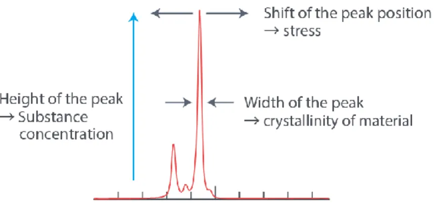
Not only is the location of the peak important, the shape of the peak is important as well. The shape helps determine the level crystallinity. The residual stress can also be determined by the direction and frequency of every Raman peak.

Figure 2.13 Raman spectrum of Ethanol

(38)

Animal Studies Conducted Prior to Experimentation

The samples used in this study originated from a previous animal study in which Yucatan miniature swine were treated with doxorubicin for 4 months and followed by cardiovascular Magnetic Resonance Imaging (CMR) in order to detect early cardiotoxicity. The protocol for the preparation and experimentation of their samples as well as ours was approved by the Comité d’éthique de protection animal at the CrCHUM.

The Sinclair Bio-Resources department located in Misouri provided seven miniature swine for the purpose of the experimentation. A silicone catheter was implanted in these infant animals via the left superior vena cava following the acclimation. All injections were administered through these vascular access ports. Five of the seven Yucatans were randomly selected to receive the doxorubicin injection while the remainder were administered with a saline solution. Once all animals were evaluated by three echocardiography and CMR, they were sacrificed. The major organs such as the liver, kidney, diaphragm, lung were preserved in liquid nitrogen before cytotoxic took effect due to the drug. Most notably, the heart was preserved for specific cardiotoxicity tests conducted by means of MRI, rheometry and Raman Spectrometry. The treatment and imaging protocols followed the guidance of Hermans and Ferrans’s study (Herman and Ferrans et al., 1983). The time elapsed for the totality of the experimentation including echocardiography evaluation and sacrificing the animals was five months.

(39)

CHAPTER 3 RHEOMETRY OF THE MYOCARDIUM

Preparation of the Samples

The samples were dissected and preserved frozen at -80°C since the previous study described in the literature review. The samples were found in various shapes (Figure 3.1) and had to be thawed in order to prepare circular shapes of 20mm diameter and 2.5mm ±0.5mm thickness.

The resulting pieces illustrated in figure 3.2 were dissected using 3D printed equipment. The preparation is described in detail in the protocol below.

Figure 3.1 Parts before the requisition of samples used for experimentation

(40)

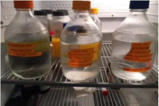
The tyrode solution, invented by Maurice Tyrode, is an isotonic solution, meaning sharing the same osmotic pressure with interstitial fluid, used in physiological experiments such as tissue

culture derived from Ringer-Locke’s solution. Its primary content is sodium (NaCl) but differs

from the Ringer-Locke’s solution in that it contains magnesium. Since the tyrode solution is

oxygenated, it helps preserve the physiological and mechanical properties of tissues irrigated in

blood. Submerging once shaped in a circular disc will allow the samples to remain hydrated and

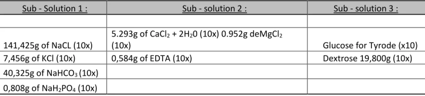
prevent them from drying out before being placed on the rheometer’s spindle. In order to realize the tyrode solution, 3 sub-solutions were prepared (Table 3.1) which, after their mixture with the proper proportions (Table 3.2), will allow us to get a fresh tyrode solution.

(41)

Table 3.1 Three sub-solutions needed to compose the Tyrode Solution

Additionally, the pH should be near neutral while taking into consideration that the pH levels are influenced by oxygenation. The resulting pH, measured by litmus paper was approximately 7.4 when preparing the tyrode solution. The slices were placed in the solution for ~ 20 minutes at room temperature to reduce shock before proceding in tissue culture validated by article (Qiao et al., 2019). To make a 1L of solution, we followed Sandstrom’s recipe procedure below:

Table 3.2 Ratio needed for the mixture of the three sub-solutions

50mL Solution

1) Mix: 100 mL of Sub-solution 1 (10 X)

800 mL of dd H2O

2) Gas with 5% CO2 for approx. 30 min to adjust pH

3) Add: 100 mL Sub-solution 2 (10X) 4) Add: 100 mL Sub-solution 3 55 mM (10x)

Sub - Solution 1 : Sub - solution 2 : Sub - solution 3 :

141,425g of NaCL (10x)

5.293g of CaCl2 + 2H20 (10x) 0.952g deMgCl2

(10x) Glucose for Tyrode (x10)

7,456g of KCl (10x) 0,584g of EDTA (10x) Dextrose 19,800g (10x)

40,325g of NaHCO3 (10x)

(42)

In order to get results as consistent and comparable as possible, the samples needed to be cut into circular shapes. To that end, we designed a slicer as a mean to place the part while pressing along the wall to perform evenly sliced samples. The holder for the peripheral cut was used afterwards to get a perfectly shaped circular disc. The CAD models of Figure 3.4 and Figure 3.5 were 3D printed.

In order to cut 5cm x 7cm samples (approximately 1/3 of each piece of miniature swine sample), we submerged a sharp knife in a beaker filled with heated water in order to penetrate the piece frozen at -80°C.

Samples were prepared two years after being sacrificied but were preserved in the freezer at -80°C. The procedure of harvesting the parts right after being sacrificed was followed and samples were prepared as for other future tests being conducted using the myocardium as the studied model. In an article written by Sirry et al., infarcted hearts were preserved as of the very first day post euthanasia (Sirry et al., 2016). Studies over the years including that of Stenman et al. studied the long term effects of tissues stored in the freeze at -80°C. The study concluded that there were no adverse effect on the tissues’ histomorphology or RNA quality (Stenman et al., 2013).

Figure 3.4 Slicer Figure 3.5 Holder for Peripheral Cut

(43)

Given that RNA is most susceptible in degradation when compared to other parts comprised in the composition of tissues and that of 153 samples studied over different period of time, no correlation with storage time was observed on the RNA quality (Stenman et al., 2013). The little to no effect on the RNA quality is emblematic to other compartments found in tissues. Though some of our samples showed slight signs of fracture, we did not fear alterations in the tissues’ histomorphological and mechanical properties. However, the paper did put a preference towards very low storage temperature in liquid nitrogen as the method of choice for long-term storage but that either method worked.

Each piece of heart was dissected in as many samples that we could obtain while remaining consistent with the diameter set out to be 20mm with an overall thickness varying from 2-3mm. For this particular research, we opted to study three myocardial regions of the heart; the left ventricle (LV), the right ventricle (RV) and the septum going running from the base of the heart to the apex. Once the cardiac pieces were cut, we preserved the cut pieces in cubes of approximately (3cm x 3cm x 3cm) at -20°C.

The slicer allows a thickness of 2,5mm ± 0,5mm and the device to host the pieces allowed for a consistent diameter cut of 20mm. The initial proposal was to cut the pieces at 25mm to match the same diameter of the spindle located on the rheometer. However, after further analyzing the available pieces, it would have been difficult to maintain a 25mm diameter when some pieces were already smaller than expected.

Samples retrieved for the experimentation can be found listed in Table 3.3. It is important to know from which part each sample was retrieved in order to determine if some of the results

(44)

obtained can be derived from the physiological properties of the miniature swine as well as if there is a common denominator for the samples found from the same part but at a different compartment of the heart. The goal is to also determine the effects a sample’s thickness has on the overall property of the myocardium tissue.

The three areas of interest are the posterior left ventricle (LV POST), the anterior left ventricle (LV ANT) and the right ventricle (RV) and the septum. The left ventricle samples were more frequently used since it comprised a larger portion of the heart allowing to retrieve more

(45)

samples. Freezing, in general, causes visible or non-visible damage using virtually any practical method. The main changes caused in samples through freezing or unfreezing are dehydration and shrinkage, some form of chemical property alteration, a change in the overall structural integrity of a sample, and/or a grave breakdown better known as the “thaw-rigor” process (B.J Luvet et al., 1964). In total, 24 samples were used, both treated and untreated. Some samples showed sign of fracture in various areas due to the extensive period of being left frozen at -80°C but were still candidates as it had negligible effects on the overall structural integrity of the samples.

Mechanical Testing Protocol

The mechanical testing protocol was composed of a strain sweep test which helped determine the optimal deformation (), a frequency sweep to determine the sample’s storage, loss modulus and complex viscosity as a function of the applied frequency and a stress-relaxation test to help calculate the relaxation modulus of the samples. Finally, a redo of the frequency sweep was conducted to determine if the sample’s storage modulus altered during the stress-relaxation test. All these tests fall under the general rheological test called oscillation experiments.

The goal for the strain sweep test using the rheometer is to determine the level of optimal deformation () to apply during the frequency sweep test to insure that the response to the shear modulus is linear throughout the frequency domain of 0,1Hz to 100Hz. We first made the assumption of a homogenous heart. To perform this stage of our tests, we made use of a pig’s heart bought at the butcher to avoid the waste of the experimentation’s actual samples. We followed the

(46)

same procedure as if we would have used the samples by placing the pieces purchased at the butcher in the CEPSUM (Centre d’éducation physique et des sports de l’université de Montréal) freezer at -80°C.

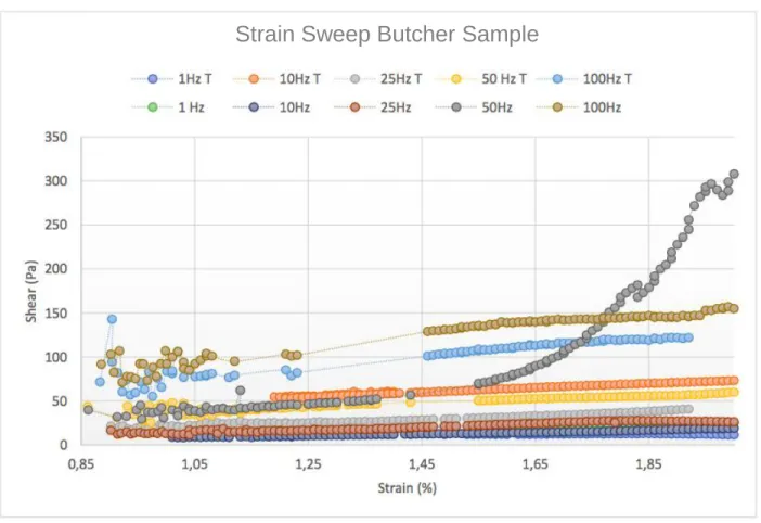
The samples used for the strain sweep were subjected to strain sweep tests varying from 1Hz, 10Hz, 25Hz, 50Hz and 100Hz on a deformation domain from 0.01% to 2%. This first step was repeated three times to insure consistent results.

(47)

Three prepared cylindrical samples on the myocardium part of the heart were submitted to 6 cycles of preconditioning at 0.1% beginning at 0.1Hz. The deformation value (=1.6%) previously found in the strain sweep was used to perform the remainder of the frequency sweep test. The frequency range was conducted from 0.1Hz to 100Hz. The frequency up until 100Hz was imposed based on 𝜔 = 16 rad.s-1 _{and it being derived from}_{𝜔 = 2πf. Refer to the graph A11 in} Appendix to further understand this frequency range.

The preliminary frequency sweep tests on the butcher samples allowed us to determine that 20 measuring points was sufficient to achieve clear curbs all while limiting the acquisition time. All tests were performed at core body temperatures (37°C). The samples were subjected to 10 cycles of preconditioning at 0.1% with a deformation =1.6%.

During the preliminary experiments, the specimen dried out quite rapidly. We originally made use of tyrode solution droplets, however, its isotonic properties caused the droplets to spread itself thin, reducing its permeability. This led us to making use of a low-viscous canola oil droplet applied on the periphery of the sample, inspired by (Nicolle, 2010) where we were able to preserve a hydrated sample all the way until the end of each test.

(48)

In addition, the viscosity of the canola oil was low enough relative to the sample that the tests were conducted in a negligible manner.

From the frequency sweep, the complex viscosity can be determined using the following formula: Complex Viscosity = viscosity – i ˣ elasticity

where i is the complex identity [42]. The overall shear modulus can be found using the following formula:

G* = G’ + iG’’

(49)

The stress-relaxation test is used to determine a sample's viscoelasticity (stress over shear rate) and modulus (stress over strain) properties when subjected to a prolonged constant strain at a constant temperature. The viscoelasticity is a property of a material that exhibits both viscous and elastic character. The stress-relaxation test helps find the stress-relaxation modulus, G, also known as the shear modulus, which is the observed decrease in stress with respect to the strain generated in the structure. Measurements of G, G’ and G’’ with respect to time, temperature, frequency and stress/strain are important in order to characterize a material’s viscoelasticity. The rate of stress of a sample to deform at a constant temperature is known as the shear rate. It is the slope created by the relaxation modulus vs. time. The reason that the stress relaxation test was chosen in this study was because the contact surface between the sample and the spindle remained constant for the entire test with a pre-set strain. Consequently, the stress is always proportional to the measured force (Cespi et al., 2007). This statement holds true only when samples are very similar in shape and size.

(50)

We reused each sample from the frequency sweep and conducted a stress relaxation test immediately after without accessing the samples in the rheometer’s compartment. Three level of deformation were originally tested: 0.2%, 0.5% and 1% with a time of relaxation of 350 to 500 seconds in between each of four ramps tested. Ultimately, after obtaining unsatisfactory graphs with these three deformation percentages, through consulting the report of (Nicolle, 2010), the deformation value for the stress relaxation test had to be equivalent to that of the frequency sweep test (=1.6%). The stress relaxation stage was repeated three times to insure consistency in the results. In total, 24 samples both treated and untreated were tested. The samples’ codes were repetition based on the preceding test conducted by Dr. Périe-Curnier and her team in Australia back in 2014.

Once the stress relaxation test was completed, we redid the frequency sweep test to make note of any variations caused by the relaxation test on the sample’s storage modulus. The test itself consisted of the same procedure found in section 3.2.2.

(51)

Mechanical Testing Results

The graph relating the shear stress as a function of the strain percentage in Figure 3.9 illustrates the curves obtained for the ten samples tested during the strain sweep. Firstly, there were no values for the deformation that were recorded below 0.8% due to the sensitivity of the machine. The second observation was that all the curves from 1Hz to 100Hz follow the same tendencies other than the curb at 50Hz which can be negated as an out of order deviation. Another observation was that in the lower strains, there were less data recorded compared to the higher strains. This greatly limited the domain of deformation values, beginning only at 1.4%. This also greatly limited the domain of values for the deformation for which we were seeking a period of linearity common to the entire curve. The frequency sweep was subdivided into two categories: the first set of frequency varying from 1Hz to 100Hz for samples submerged in the tyrode solution denoted by the letter “T.” The 2nd_{category were samples placed directly under the spindle after slicing. The} goal for this was to determine how the composition of the solution would affect the shear properties of the results.

(52)

The strain sweep test allowed us to retain two sets of deformation that were used to conduct the frequency sweep. The first set of values varied from [1.7-1.9] % (Figure 3.10) and the second set being [1.5-1.7] % (Figure 3.11) as the goal of the R regression was to get closest to the value of 1,00.

Strain Sweep Butcher Sample

(53)

We still observe through Figure 3.11 as we do in Figure 3.10 another out of order regression this time for the frequency equal to 1Hz. If it is excluded from the data results, we obtain a regression coefficient of average value equal to 0.954 in Figure 3.10 whereas an average regression value of 0.9722 was observed in Figure 3.11, which is more of an acceptable value.

(54)

To conclude, though the second set of linearity conducted achieved similar regression coefficient averages than that of the interval [1.7 to 1.9]%, by force of an iterative approach, the deformation value of  =1.6% was retained for the following frequency sweep. This deformation percentage is important as it will serve as the benchmark deformation value throughout the experimentation with the miniature swine samples.

(55)

After the five samples underwent six cycles of test, we generated graph 3.12, 3.13 and 3.14 at a deformation of 1.6% which displays the butcher samples’ storage modulus, loss modulus and complex viscosity. We limited the study to collect all data points for all modulus’ until 100Hz.

0,00E+00 1,00E+03 2,00E+03 3,00E+03 4,00E+03 5,00E+03 0 20 40 60 80 100

Overview Storage Modulus Obtained From Frequency Sweep

Storage Modulus (test 1) [Pa] Storage Modulus (test 2) [Pa] Storage Modulus (test 3) [Pa] Storage Modulus (test 4) [Pa] Storage Modulus (test 5) [Pa] Storage Modulus (test 6) [Pa]

(56)

0,00E+00 2,00E+02 4,00E+02 6,00E+02 8,00E+02 1,00E+03 1,20E+03 1,40E+03 1,60E+03 1,80E+03 0 20 40 60 80 100

Overview Loss Modulus Obtained From Frequency Sweep

Loss Modulus (test 1) [Pa] Loss Modulus (test 2) [Pa] Loss Modulus (test 3) [Pa] Loss Modulus (test 4) [Pa] Loss Modulus (test 5) [Pa] Loss Modulus (test 6) [Pa] 0,00E+00 1,00E+03 2,00E+03 3,00E+03 4,00E+03 5,00E+03 0 20 40 60 80 100

Overview Complex Viscosity Obtained From Frequency Sweep

Complex Viscosity (test 1) [Pa·s] Complex Viscosity (test 2) [Pa·s] Complex Viscosity (test 3) [Pa·s] Complex Viscosity (test 4) [Pa·s] Complex Viscosity (test 5) [Pa·s] Complex Viscosity (test 6) [Pa·s]

Figure 3.14 Complex Viscosity Frequency Sweep Test on Butcher Samples

(57)

We achieved a frequency up to 100Hz during these test described in Figure 3.12, 3.13 and 3.14. Based on the data values obtained, we were able to trace the average and standard deviation value of G’, G’’ and of the complex viscosity for the five additional butcher sample tests. The storage modulus, G’, in viscoelastic materials is a measure of the elastic response of a material which means that it measures the material’s ability to store energy (Kalyanamaran et al., 2012). The higher the storage modulus, the more the material will be considered « solid » and will thus have a lower capacity to deform. The loss module, G’’, also known as the viscous modulus is the ability for a material to dissipate energy such as heat (Kalyanamaran et al., 2012). The complex viscosity, η, describes the resistance for matter to flow. It is the relationship between the shear viscosity as a function of the material’s shear rate (Kalyanamaran et al., 2012).

-5,00E+00 1,95E+02 3,95E+02 5,95E+02 7,95E+02 9,95E+02 1,20E+03 1,40E+03 1,60E+03 1,80E+03 0 20 40 60 80 100

Values of G', G'' and η for Frequency Sweep  = 1.6%

Storage Modulus Average [Pa] Loss Modulus Average [Pa·s] Complex Viscosity Average [Pa]

(58)

The average and standard deviation combined for all three parameters interested in the study of the butcher samples can be found in Figure 3.15. The graph was derived from the individual graphs obtained for the storage modulus, loss modulus and complex viscosity.

Based on the tendencies of Figure 3.16, even though the results for the untreated hearts obtained are of a factor 1.4 times the amount of the butcher samples, the graph tendencies remain nearly similar. The average storage modulus for the untreated test samples tend to converge between 3.50E+03 and 4.00E+03 whereas the average storage modulus for the butcher samples had a tendency for a steady increase (slope  16) after 40 seconds. The average value of the data points found in the untreated samples curve was of 3.46*103 and the average value for the data points found in the butcher samples was 4.9*103. This allowed us to closely compare the samples from the butcher to the untreated samples due to the lack of samples retrieved.

0,00E+00 1,00E+03 2,00E+03 3,00E+03 4,00E+03 5,00E+03 0 20 40 60 80 100 St or ag e M od u lu s (P a) Angular Frequency (1/s)

Average Frequency Sweep  = 1,6%

Average Frequency Sweep Butcher Average Untreated Test Samples

(59)

i) Left Ventricle

The samples used can be consulted in Table 3.3. Based on Figure 3.17, we observed a higher storage modulus on average for DOXO samples denoted by the circular data point than we did for untreated samples. However, regardless of if the sample was treated or untreated with doxorubicin, both displayed similar storage modulus tendencies studied during the frequency sweep. The last item to observe from Figure 3.17 is that the posterior samples obtained a higher standard deviation (longer vertical error bar) than the anterior samples. There was an insufficient amount of samples

0,00E+00 5,00E+02 1,00E+03 1,50E+03 2,00E+03 2,50E+03 3,00E+03 3,50E+03 0 10 20 30 40 50 60 70 80 90 100 St or ag e M od u lu s (P a) Angular Frequency (1/s)

Frequency Sweep Left Ventricle

Average Posterior LV DOXO Average Posterior LV UNTREATED Average Anterior LV DOXO Average Anterior LV UNTREATED Figure 3.17 Average Storage Modulus results for the Left Ventricle Samples

(60)

to calculate the standard deviation for the untreated samples, which explain why the triangular data points did no display vertical error bar marking its sample’s standard deviation. To view the results for each sample code from Table 3.3 covering the left ventricle, the graph can be consulted in Appendix A, Figure A1 & A2.

The results for the complex viscosity found in Figure 3.18 draw inconclusive results. The only pertinent information to note is of the similar complex viscosity found in both the untreated and DOXO samples which seems to be unaltered.

0,00E+00 5,00E+02 1,00E+03 1,50E+03 2,00E+03 2,50E+03 0 20 40 60 80 100 120 140 C om p le x V isc osit y [P a] Angular Frequency (1/s) Frequency Sweep Left Ventricle

Average Posterior LV DOXO Average Posterior LV UNTREATED

Average Anterior LV DOXO Average Anterior LV UNTREATED

(61)

Figure 3.19 Average loss modulus for Left Ventricle Samples

The last measurement of interest is the loss modulus found in Figure 3.19. When combining all samples studied for the posterior and anterior left ventricles, we notice an increase in the loss modulus for the DOXO samples compared to the untreated samples. This result for the left ventricle is in line with the results obtained for the storage modulus.

0,00E+00 1,00E+02 2,00E+02 3,00E+02 4,00E+02 5,00E+02 6,00E+02 7,00E+02 8,00E+02 0 10 20 30 40 50 60 70 80 90 100 Loss M od u lu s (P a.s) Angular Frequency (1/s)

Frequency Sweep Left Ventricle

Average Posterior LV DOXO Average Posterior LV UNTREATED

(62)

ii) Septum

Contrary to the left ventricle, the testing for the samples covering the septum show a diminishment of the storage modulus and loss modulus in those carrying the doxorubicin injection. The untreated samples exhibited an average storage modulus of 3.165*103 Pa whereas the DOXO samples averaged 2.095*103 _{Pa. This represents a 33% drop in the DOXO sample’s viscoelastic} ability to absorb energy. These results are retrieved from the tables found in Appendix B. Given the insufficient data can thus conclude that the doxorubicin agent has a greater negative impact in the septum in the mechanical properties than in the left ventricle. To view the results obtained for each sample code, a graph displaying the following for the septum samples in Appendix A, Figure A8. 5,00E+02 1,00E+03 1,50E+03 2,00E+03 2,50E+03 3,00E+03 3,50E+03 4,00E+03 0 10 20 30 40 50 60 70 80 90 100 St or ag e M od u lu s (P a) Angular Frequency (1/s) Frequency Sweep SEPTUM

Average SEPTUM DOXO Average SEPTUM UNTREATED

(63)

Figure 3.21 Average Complex Viscosity Frequency Sweep Septum

Similarly to the Complex Viscosity of the left ventricle, Figure 3.21 shows inconclusive results but both induced and non-induced samples had nearly identical complex viscosities. They were comparable in that they both outputted a rational function allure where samples converged to a complex viscosity almost immediately after we started collecting data points. This curve occurred not only for the septum but for the left and right ventricles as well.

0,00E+00 5,00E+02 1,00E+03 1,50E+03 2,00E+03 2,50E+03 3,00E+03 3,50E+03 4,00E+03 4,50E+03 0 100 200 300 400 500 600 700 C om p le x V isc osit y (P a) Angular Frequency (1/s) Frequency Sweep Septum