Validation de l’utilisation d’indicateurs physiologiques de stress comme indicateurs de qualité des habitats

Université de Montréal

Validation de l’utilisation d’indicateurs physiologiques de stress comme indicateurs de qualité des habitats

Cédric Lejeune

Département des Sciences biologiques de l’Université de Montréal Faculté des arts et des sciences

Mémoire présenté en vue de l’obtention du grade de Maîtrise ès sciences (M.Sc) en sciences biologiques

Janvier 2018

i

Résumé

Le développement de modèles de qualité des habitats est souvent limité par notre incapacité à lier les processus à l’échelle des écosystèmes au succès écologique des individus. Les indicateurs physiologiques de stress ont été proposés comme une méthode

complémentaire aux approches classiques de modélisation de la qualité des habitats basées sur des indicateurs d’utilisation des habitats. Néanmoins, l’utilisation d’indicateurs physiologiques associés au stress comme outil de modélisation de qualité des habitats n’a pas encore été rigoureusement validée. Les échelles temporelles pour lesquelles les indicateurs de stress constituent potentiellement le lien entre processus écosystémiques et le succès écologique sont encore inconnues. Dans le but de contribuer à la validation de ces indicateurs, les niveaux de bases et réponses du cortisol, du glucose et du lactate ont été mesurés chez 323 bec-de-lièvres (Exoglossum maxillingua) situés dans 3 différentes rivières des Laurentides (Québec, Canada) durant l’été 2016. Ces indicateurs de stress ont par la suite été liés aux caractéristiques de l’environnement et à deux facteurs de conditions utilisés pour évaluer le succès écologique des individus. Les résultats obtenus démontrent qu’il serait possible d’utiliser les niveaux réponses de glucose pour modéliser la qualité des habitats à de courtes échelles temporelles.

Mots-clés : Indicateurs de stress, Cortisol, Glucose, Lactate, Qualité des habitats,

ii

Abstract

Stress-related physiological indicators have been proposed as an alternative approach to model habitat quality due to their relation to an individual’s fitness. However, the

validation of this approach is far from complete since the temporal scales at which

physiological indicators are related to local environmental characteristics and are a predictor of fish fitness has not been assessed. Thus, the goal of this study was to further explore the potential of physiological indicators in facilitating the development of habitat quality models. To achieve that, the basal and response levels of cortisol, glucose and lactate in the blood were assessed in cutlip minnows (Exoglossum maxillingua) located in three different Laurentian rivers (Quebec, Canada) from July to August 2016. Those indicators were then linked to the assessed environmental characteristics and to two condition factors used to represent fish fitness (whole-body lipid concentration and LeCren condition factor) with models built through a two-stage hybrid variable selection procedure using ridge and LASSO type penalties. Our results suggest that response levels of blood glucose depend strongly on the local environmental characteristics and are good predictors of the fish’s lipid concentration validating their potential use at the daily temporal scale as habitat quality indicators.

iii

Table des matières

Résumé ... i 

Abstract ... ii 

Table des matières... iii 

Liste des tableaux ... iv 

Liste des sigles et abréviations ... vi 

Remerciements ... viii 

Introduction générale ... 1 

Les approches de modélisation de la qualité des habitats ... 1 

La réponse au stress chez les poissons ... 2 

Les indicateurs physiologiques, le succès écologique et la qualité des habitats ... 6 

La validation de l’utilisation d’indicateurs physiologiques de stress pour modéliser la qualité des habitats ... 8 

Contributions des différents auteurs à l’article ... 10 

Validation of Indicators of Organismal Physiological Status to Model Fish Habitat Quality .. 11 

Abstract ... 12 

Introduction ... 13 

Material and Methods ... 20 

Study Sites ... 20 

Study Species ... 22 

Fish Sampling ... 22 

Surveys of Environmental Characteristics ... 24 

Laboratory Analysis ... 25 

Computations and Statistical Analysis... 26 

Results ... 31 

Variation in Environmental Characteristics ... 31 

Variation in Physiological Indicators... 31 

Relationship between Physiological Status and Environmental Characteristics ... 35 

Relationship between Conditions Factors, Physiological Status and Environmental Characteristics ... 36 

Quantifying the Relative Contribution of Physiological Indicators and Environmental Characteristics in Explaining Condition Factors ... 39 

Discussion ... 43 

Relationship between Physiological Status and Environmental Characteristics ... 43 

Relationship between Conditions Factors, Physiological indicators and Environmental Characteristics ... 45 

Quantifying the Relative Contribution of Physiological Indicators and Environmental Characteristics in Explaining Conditions Factors ... 49 

Habitat Modeling Using Physiological Indicators ... 49 

Discussion générale ... 52 

Bibliographie... ix 

iv

Liste des tableaux

Table I : Surveyed environmental characteristics used to study their effect on fish

physiological indicators. For each environmental characteristic, the instrument or method used is given, as well as a general hypothesis of how it could affect fish stress. ... 25

Table II : Mean standard deviation (SD), minimum value and maximum value of

environmental characteristics distribution by sampling day. Since the presence of rain was observed only 3 times during sampling, it was omitted from the table. ... 32

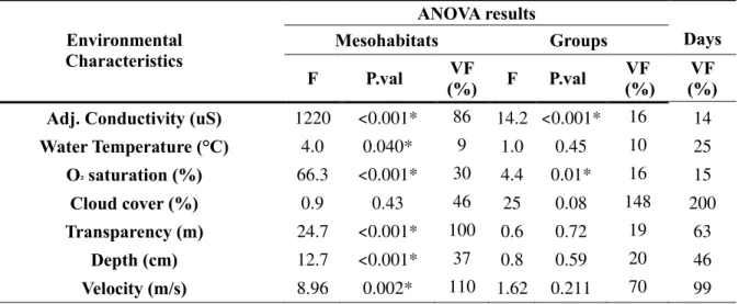
Table III : ANOVA results (F statistic, P.values and Variation factor in %) for variation across mesohabitats and groups of consecutive sampling days of environmental characteristics. Statistically significant P.values are marked with an *. ... 33

Table IV : Mean, standard deviation (SD), minimum value and maximum value of

physiological indicators and condition factors of all fish. ... 33

Table V : ANOVA results (F statistic, P.val. and Variation factor in %) for variation across mesohabitats and groups of consecutive sampling days of physiological indicators and condition factors using means per sampling day. Statistically significant P.values are marked with an *. ... 34

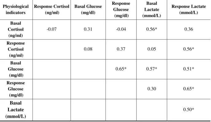
Table VI : Pearson’s correlation coefficients for each physiological indicator using the means of each sampling days. Significant correlations (p<0.05) are marked with an asterisk (*). ... 34

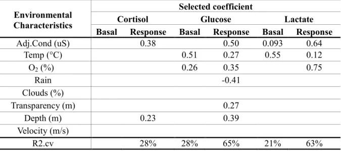
Table VII : Selected coefficients and cross-validated R2 _{for the LASSO models relating scaled}

physiological indicators with scaled environmental characteristics. Only values greater than zero are shown. ... 36

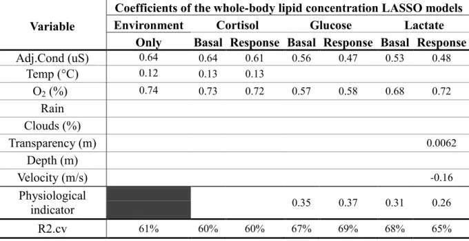
Table VIII: Coefficients of the LASSO models relating whole-body lipid concentration with scaled physiological indicators and scaled environmental characteristics. Only values greater than zero are shown. No physiological indicators were used to predict whole-body lipid concentration in the environment only model represented in the first column. In the other six models, environmental characteristics and each physiological indicator were used as

v

Table IX : Coefficients of the LASSO models relating scaled LeCren condition factor with scaled physiological indicators and scaled environmental characteristics. Only values greater than zero are shown. No physiological indicators were used to predict whole-body lipid concentration in the environment only model represented in the first column. In the other six models, environmental characteristics and each physiological indicator were used as

explanatory variables conjointly. ... 39

Table X: Variation partitioning for the LASSO models relating scaled whole-body lipid concentration with scaled environmental characteristics and physiological indicators. Only values greater than zero are shown. The A fraction corresponds to the variation explained exclusively by each physiological indicator, the B fraction corresponds to the variation explained conjointly by environmental characteristics and physiological indicators and the C fraction corresponds to the variation explained exclusively by environmental characteristics. 42

Table XI : Variation partitioning for the LASSO models relating scaled LeCren condition factor with scaled environmental characteristics and scaled physiological indicators. The A fraction corresponds to the variation explained exclusively by each physiological indicator, the B fraction corresponds to the variation explained conjointly by environmental characteristics and physiological indicators and the C fraction corresponds to the variation explained

exclusively by environmental characteristics. ... 42

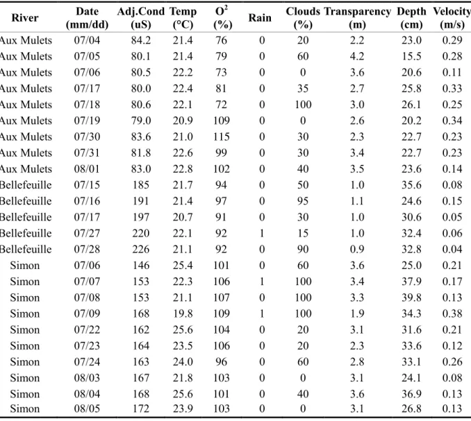
Table XII : Adjusted water conductivity (uS), water temperature (°C), O2 _{saturation (%),}

presence of rain (0 = no rain, 1 = rain) , cloud cover (%), water transparency (m) values for each sampling day and mean of 10 random stratified measurement of water column depth (cm) and velocity (m/s) for each sampling days. ... xvi

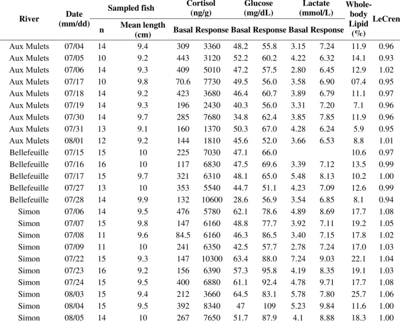
Table XIII : Mean per sampling day of basal and response levels of cortisol, glucose and lactate, whole-body lipid concentration and LeCren condition factor. Due to unforeseen shipping issue, lactate values are not available for one sampling days and are represented by empty cells. ... xvii 

vi Liste des figures

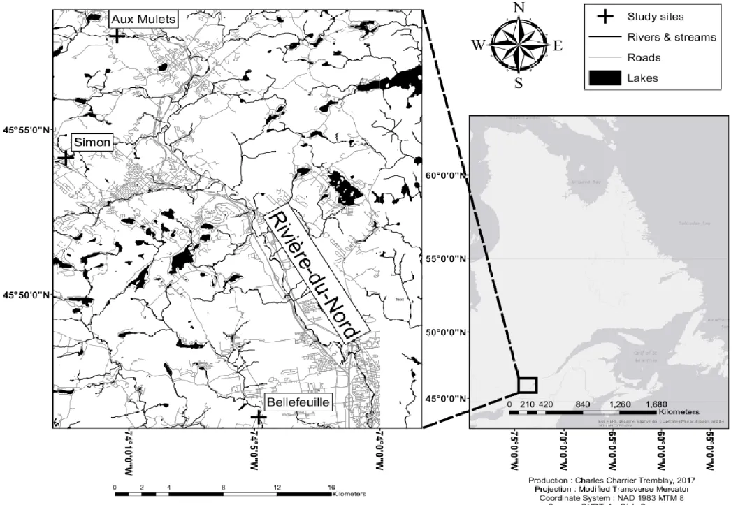
Figure 1: Map of the sampled sites ... 21

Liste des sigles et abréviations

ELISA : Enzyme-linked immuno-sorbent assay (Dosage d'immunoabsorption par enzyme liée) HHI : Axe hypotalamo-hypophysaire-interrénalien.

HSC : Axe hypotalamo-sympathique-chromaffine.

OLS : Ordinary least square (Méthode des moindres carrés ordinaire)

NADH et NAD+_{: Nicotinamide adenine dinucleotide (Nicotinamide adénine dinucleotide)}

P.val : Probability value (Valeur de probabilité)

vii À Aldo Leopold

viii

Remerciements

Je voudrais commencer par offrir de sincères remerciements à Daniel Boisclair, mon directeur de maîtrise, de m’avoir offert toute sa confiance et épaulé durant cette aventure. Merci à Steven J. Cooke pour ses excellents conseils tout au long du projet. Je voudrais aussi souligner la généreuse contribution de M. Tony DiPaolo. Grâce à une bourse d’études et une subvention, il a su supporter mes études et la réouverture de l’aquarium du département. Merci à l’ensemble de l’équipe du laboratoire Daniel Boisclair qui étaient présents lors de mon passage : Emmanuelle Chrétien, Caroline Senay, Guillaume Guénard, Simonne

Harvey-Lavoie, Camille Macnaughton, Joanie Asselin, Guillaume Bourque, Gabriel Lanthier, Cynthia Guéveneux-Julien et Tom Bermingham; j’ai eu énormément de plaisir à apprendre à vous connaître, à rire, échanger et partager avec vous. Vous avez toujours pris le temps de répondre à mes questions et de m’encourager. Je n’aurais pas pu mieux tomber. Merci à Guillaume Guénard de m’avoir aidé avec les modèles statistiques et merci à Charles Charrier-Tremblay d’avoir produit la carte des sites et d’avoir partagé mon amour des poissons. Je voudrais aussi souligner le précieux travail que Baptiste Thevenet, Christophe Benjamin et Caroline Fink-Mercier ont effectué avec moi sur le terrain lors de la prise de données. Un grand merci à l’ensemble de mes collègues de l’AECBUM, à l’équipe administrative et technique du département et à tous ceux qui m’ont encouragé durant le projet.

1

Introduction générale

Les approches de modélisation de la qualité des habitats

La destruction, la fragmentation et l’altération des habitats font partie des menaces les plus importantes à la biodiversité mondiale (Brooks, 2006; Hanski, 2011; Mantyka-Pringle, 2012). Les actions de conservation et de protection des populations menacées sont souvent limitées par la difficulté de modéliser la capacité d’un habitat à assurer la survie et la

reproduction des populations le fréquentant (Cooke, 2008). Cette capacité, appelée qualité des habitats, est le plus souvent modélisée chez les poissons à l’aide d’approches se basant sur l’utilisation des habitats en raison de leur faible coût et leur relative simplicité (Johnson, 2007). Ces approches supposent une relation positive entre les indicateurs d’utilisation comme la présence, l’abondance, la biomasse ou le mouvement des organismes (Johnson, 2007; Van Horne, 1983) et la qualité de l’habitat. Cette relation peut être causée par le déplacement volontaire des poissons d’un habitat de faible qualité vers des habitats de plus grande qualité ou par un plus grand succès écologique des individus fréquentant les habitats de meilleure qualité (Chalfoun, 2007; Morris, 2003; Remes, 2000). Cependant, ces modèles semblent échouer dans plusieurs contextes à identifier les paramètres environnementaux déterminant la qualité des habitats. Une des raisons avancées pour expliquer ces échecs est qu’ils ne prennent pas en compte les processus se déroulant à l’échelle des individus (Horodysky, 2015). Dans un contexte de changements globaux, l’identification de ces processus s’avère primordiale pour soutenir les efforts de conservation (Seebacher, 2012).

2

Ces dernières années, un nombre important d’études (Cooke, 2010; Horodysky, 2015; Lennox, 2018; Mckenzie, 2016; Seebacher, 2012; Wikelski, 2006; Young, 2006) avancent que des modèles de qualité des habitats incluant la physiologie des individus permettraient de pallier aux faiblesses des modèles d’utilisation des habitats. Ces modèles seraient en mesure d’offrir des mécanismes concrets liant environnement, individus et population à travers le succès écologique ou « fitness » des organismes étant donné que les processus physiologiques sont, d’une certaine manière, la courroie de transmission entre l’environnement et le succès écologique des individus (Feder, 2000; Horodysky, 2015; Huey, 1991). De récentes études suggèrent que des indicateurs physiologiques associés à la réponse au stress seraient potentiellement de bons indicateurs de la qualité des habitats chez les poissons puisque les voies métaboliques associées au stress jouent le rôle d’intermédiaires entre l’environnement et la physiologie interne de l’organisme (Belanger, 2017; Blevins, 2013; Lennox, 2018;

O’Connor, 2010; Pottinger, 2011).

La réponse au stress chez les poissons

Lorsqu’un organisme fait face à un évènement menaçant son équilibre interne appelée homéostasie (Cannon, 1929), il doit dépenser une certaine quantité d’énergie pour conserver cet équilibre. L’énergie que l’organisme doit dépenser pour conserver son homéostasie dans un environnement donné est appelée charge allostasique (Romero, 2009). Pour rétablir l’équilibre interne, une série de réactions physiologiques appelée réponse au stress est sollicitée. Cette réponse, dont les mécanismes ont fortement été conservés au cours de

l’évolution (Bonier, 2009; Denver, 2009), peut être divisée en trois différentes étapes chez les vertébrés : la réponse primaire, secondaire et tertiaire (Barton, 2002).

3

La réponse primaire au stress implique deux voies métaboliques différentes: la voie adrénergique associée aux hormones catécholamines et la voie glucocorticoidienne associée aux hormones corticostéroïdiennes (Barton, 2002). Elles sont contrôlées respectivement chez les poissons par l’axe hypothalamo-sympatique-chromaffine (HSC) et l’axe hypotalamo-hypophysaire-interrénalien (HHI).

La réponse primaire au stress pour l’axe HSC commence avec le relâchement dans le sang des hormones catécholamines, soit l’épinéphrine et la norépinephrine aussi appelées adrénaline et noradrénaline. Elles sont relâchées à partir des cellules chromaffines situées dans les tissus interrénaux des poissons aussitôt que le stress est perçu. Contrairement aux autres vertébrés, les poissons et amphibiens n’ont pas de glandes surrénales à proprement parler. Ainsi, les cellules chromaffines sont distribuées dans le rein au lieu de former une glande distincte (Barton, 1998). Le relâchement des hormones catécholamines est régulé par stimuli nerveux provenant des fibres cholinergiques préganglionaires du système nerveux

sympathique, par des facteurs hormonaux comme la concentration de catécholamines ou de cortisol et par des facteurs non hormonaux comme la concentration dans le plasma d’ions potassium, de CO2 et d’O2(Randall, 1992). Les principaux effets de cette famille d’hormones

sont l’augmentation de la glycémie dans le sang, de la ventilation, de la circulation sanguine et de l’apport en oxygène aux tissus (Bonga, 1997; Fabbri, 2016). Toutefois, l’utilisation des hormones catécholamines est assez rare en modélisation physiologique de la qualité des habitats puisque leurs niveaux augmentent rapidement (<1min) après la perception d’un stress comme la capture ou un prélèvement sanguin et leurs effets directs sur la réponse au stress sont de courte durée (Bonga, 1997; Koolhaas, 2011).

4

Le cortisol, principale hormone glucocorticoidiennes chez les poissons, est relâché par les tissus interrénaux comme les hormones catécholamines. Cette libération est régulée par deux différentes hormones issues de l’hypophyse; la corticotropine (CRH) et

l’adrénocorticotropine (ACTH) (Barton, 2002; Bonga, 1997). Le rôle du cortisol dépend de sa concentration. À faible concentration, il est impliqué chez les poissons dans l’attribution des acides aminés à différentes voies métaboliques non protéiques, l’osmorégulation, la croissance et la reproduction (Mommsen, 1999). À forte concentration, le rôle principal du cortisol est l’activation de la glycogénolyse dans le foie permettant la libération de glucose dans le sang, mais participe aussi à la modulation du rythme cardiaque et de la ventilation (Martinez-Porchas, 2009; Pankhurst, 2011). Suite à un stress, l’augmentation de la concentration du cortisol dans le sang est observée à partir de trois minutes (Romero, 2005). Il est donc possible d’évaluer, à l’aide d’un protocole de prélèvement approprié, les niveaux de cortisol avant et après un stress.

La réponse secondaire correspond à des changements métaboliques induits par la réponse primaire. Elle est caractérisée par des changements au niveau de métabolites comme le glucose et le lactate, la production de protéines de choc thermique et des changements relatifs à l’osmorégulation (Barton, 2002). Plus spécifiquement, le glucose est le principal responsable de l’apport en énergie dans les tissus de l’organisme et les deux voies associées à la réponse primaire au stress mènent à sa libération (Barton, 2002). Cette libération semble plus être contrôlée par la voie adrénergique que par la voie glucocorticoidienne (Pankhurst, 2011). De plus, il existe un système de rétroaction négative où l’augmentation de la glycémie sanguine a tendance à réduire la glycogénolyse dans le foie (Polakof, 2008a).

5

Le lactate est aussi un produit de la réponse secondaire au stress chez les poissons. Lors d’un stress, leur consommation en oxygène a tendance à être plus grande que leur capacité d’en capter de l’environnement. Face à une importante demande énergétique et une concentration d’oxygène limitante, le pyruvate, au lieu d’être transformé en acétyl-CoA, va être réduit en lactate. Normalement, le NADH est oxydé dans la mitochondrie à l’aide de l’oxygène, mais en absence de celui-ci, cette réaction est impossible. À la place, c’est le pyruvate qui va jouer le rôle d’accepteur d’électron. Celui-ci va accepter l’électron du NADH qui va devenir NAD+_{. Cette réaction permet, en absence d’oxygène, la régénération du NAD}+_,

molécule essentielle à la production d’ATP (Facey, 2013). Toutefois, le lactate n’est pas seulement un déchet métabolique. Il peut aussi être utilisé comme source d’énergie et comme précurseur à la synthèse de glycogène (Chatham, 2002; Omlin, 2014; Polakof, 2008a).

Finalement, la réponse tertiaire correspond à des changements au niveau de

l’organisme comme la perte de masse musculaire, la réduction de la croissance, une réduction au niveau du système immunitaire et des changements dans le comportement. Ces

changements peuvent avoir des conséquences importantes sur l’organisme et peuvent réduire fortement son succès écologique (Barton, 2002, 1987; Schreck, 2001).

6

Les indicateurs physiologiques, le succès écologique et la qualité des habitats

L’information apportée par ces différents indicateurs physiologiques associés à la réponse au stress dépend du moment du prélèvement. Ainsi, pour le cortisol, les niveaux de base (ou niveaux naturels), mesurés moins de trois minutes après la capture, reflètent généralement la charge allostatique actuelle de l’environnement sur l’organisme (Bonier, 2009). Les niveaux réponses, définis comme le niveau maximal atteint après un stress aigu (généralement après 30min), reflètent la capacité d’un organisme à faire face à un stress (Barton, 2002). Ainsi, il est généralement supposé que la relation entre les niveaux de base du cortisol et le succès écologique des individus est négative. Plus la charge allostatique sur l’individu est grande, moins celui-ci sera en mesure de contribuer à la génération suivante (Bonier, 2009). Pour les niveaux réponses de cortisol, il est généralement supposé que leur relation avec le succès écologique des individus est positive. Plus un organisme est en mesure d’activer les axes associés à la réponse au stress lors d’un évènement stressant, plus il est probable que celui-ci soit capable de faire face à la charge allostatique de son environnement et ainsi être en mesure de contribuer à la génération suivante (Barton, 2002; Breuner, 2008). De plus, une activation fréquente de la réponse au stress causée entre autres par une grande charge allostatique entraine l’habituation au stress. L’habituation est un mécanisme adaptatif caractérisé par une réduction de l’intensité de la réponse (Barton, 1987; Koolhaas, 2011; Rich, 2005). Elle permettrait de réduire les effets néfastes d’une constante activation de la réponse au stress tel que la suppression du système immunitaire, du système reproducteur et de la croissance (Rich, 2005). Il n’existe donc pas de bonne ou de mauvaise réponse au stress, mais plutôt des répondes typiques d’environnements associés à de petites ou de grandes charges allostatiques.

7

Pour les niveaux de glucose dépendent en partie de la concentration en cortisol. Il serait donc possible de supposer que les niveaux de bases, comme ceux du cortisol, sont associés négativement au succès écologique et que les niveaux réponses y soient associés positivement. Similairement, des niveaux de bases de lactates élevés suggéreraient une charge allostatique élevée donc une relation négative avec le succès écologique. Des niveaux

réponses élevés suggéraient une bonne capacité à répondre à un stress et donc un meilleur succès écologique. Certaines méta-analyses ont néanmoins soulevé des incohérences entre les niveaux de cortisol et le succès écologique (Bonier, 2009; Breuner, 2008). Il semblerait ainsi que la réponse au stress est modulée par d’autres facteurs que la concentration de cortisol dans le sang tel que la concentration de récepteurs cellulaires associés à la réponse au stress ou à la concentration de globulines liant le cortisol (Breuner, 2008, 2006).

Pour être en mesure d’utiliser les niveaux de base et réponses du cortisol, du glucose et du lactate pour modéliser la qualité des habitats, certaines informations manquent encore. En effet, les échelles temporelles auxquelles les indicateurs physiologiques de stress sont associés aux caractéristiques de l’environnement et auxquels les indicateurs physiologiques de stress prédisent le succès reproducteur des individus sont encore inconnues. Dans l’éventualité où cette échelle temporelle est très grande (ex. années), il serait impossible d’utiliser les

indicateurs physiologiques de stress pour modéliser des variations de qualité des habitats à des échelles plus petites (ex. semaines). Inversement, si cette échelle temporelle est petite (ex. jours), il serait possible d’utiliser les indicateurs de stress pour modéliser des variations de qualité des habitats à de petites (ex. jours) et grandes échelles (ex années).

8

La validation de l’utilisation d’indicateurs physiologiques de stress pour

modéliser la qualité des habitats

Quelques études ont été en mesure d’associer des indicateurs physiologiques de stress avec des caractéristiques environnementales en milieu naturel à travers le temps, mais

seulement à de longues et moyennes échelles temporelles. Par exemple, une étude Pottinger, 2011 a réussi à détecter des différences entre les niveaux réponses de cortisol et de lactate selon un gradient de pollution chez l’épinoche à trois épines à travers plusieurs années. Une autre étude, Liss, Sass, & Suski, 2014 a réussi à modéliser la variation des niveaux de bases de cortisol et de glucose à l’aide des caractéristiques de l’environnement chez la carpe

argentée (Hypophthalmichthys molitrix, Valenciennes 1844) entre différents mois d’une même saison. Au niveau du lien entre les indicateurs physiologiques de stress et succès écologique, une étude O’Connor, 2010 a démontré que l’implantation d’une capsule contenant du cortisol dans des achigans à grande bouche (Micropterus salmoides, Lacépède, 1802) réduisait leur capacité à survivre à des conditions d’anoxie hivernale.

Il existe plusieurs lacunes au niveau de la validation de l’utilisation des indicateurs physiologiques de stress comme outil de modélisation de qualité des habitats. L’ensemble des études recensées liant l’environnement aux indicateurs physiologiques associés à la réponse au stress se déroulent à de longues échelles temporelles et n’incluent pas des mesures de succès écologiques. De comprendre comment ces indicateurs interagissent à de courtes échelles temporelles avec l’environnement et d’évaluer s’ils sont effectivement liés au succès écologique des individus est nécessaire avant de pouvoir les utiliser comme outil de

9

modélisation de qualité des habitats. Conséquemment, l’objectif de la présente étude vise à contribuer à la validation de l’utilisation d’indicateurs associés à la réponse au stress comme indicateurs de qualité des habitats dans le but de mieux comprendre la relation entre la physiologie des organismes et leur habitat afin de contribuer au développement de nouveaux outils en conservation. Plus précisément, notre étude vise à évaluer l’existence d’un lien à l’échelle du jour entre les caractéristiques environnementales, les niveaux de bases et réponses de cortisol, de glucose et de lactate et deux facteurs de conditions utilisés pour évaluer le succès écologique des organismes soit le pourcentage de gras total et le facteur de condition de LeCren chez le bec-de-lièvre (Exoglossum maxillingua, Lesueur 1817).

10

Contributions des différents auteurs à l’article

La conception et la réalisation de la présente étude sont un travail original de Cédric Lejeune sous la supervision des coauteurs de l’article soit Daniel Boisclair et Steven J. Cooke. L’analyse des données a été faite par Cédric Lejeune. L’écriture de l’article a été faite par Cédric Lejeune avec révisions et contributions de Daniel Boisclair.

11

Validation of Indicators of Organismal Physiological Status

to Model Fish Habitat Quality

Cédric Lejeune¹, Steven J. Cooke2 _{and Daniel Boisclair¹}

¹ Département de Sciences Biologiques, Université de Montréal, Pavillon Marie-Victorin, 90 avenue Vincent-d’Indy, Québec H2V 2S9, Canada.

² Fish Ecology and Conservation Physiology Laboratory, Department of Biology and Institute of Environmental Science, Carleton University, 1125 Colonel By Drive, Ottawa, ON K1S 5B6, Canada.

12

Abstract

Stress-related physiological indicators have been proposed as an alternative approach to model habitat quality due to their relation to an individual’s fitness. However, the

validation of this approach is far from complete since the temporal scales at which

physiological indicators are related to local environmental characteristics and are a predictor of fish fitness has not been assessed. Thus, the goal of my study was to further explore the potential of physiological indicators in facilitating the development of habitat quality models. To achieve that, the basal and response levels of cortisol, glucose and lactate in the blood were assessed in cutlip minnows (Exoglossum maxillingua) located in three different Laurentian rivers (Quebec, Canada) from July to August 2016. Those indicators were then linked to the assessed environmental characteristics and to two condition factors used to represent fish fitness (whole-body lipid concentration and LeCren condition factor) with models built through a two-stage hybrid variable selection procedure using ridge and LASSO type penalties. Our results suggest that response levels of blood glucose depend strongly on the local environmental characteristics and are good predictors of the fish’s lipid concentration validating their potential use at the daily temporal scale as habitat quality indicators.

13

Introduction

The destruction and modification of habitats have been identified as major threats to the persistence of many species around the globe (Brooks, 2006). The capacity of conservation scientists to quantify and predict the consequences of habitat alteration is impeded by the lack of understanding of the linkage between the determinants of species perpetuation and

environmental characteristics (Horodysky, 2015; Ricklefs, 2002). Habitat-based conservation, which hinges on relationships between metrics of species perpetuation (fitness metrics such as reproduction, growth, and survival rates) and environmental characteristics is one of the most common approaches used to quantify the consequences of habitat alteration on species (Huey, 1991; Primack, 2012). The development of such relationships, hereafter referred to as “habitat quality models” (Hall, 1997) is hampered by the mismatch between the spatial and temporal scales at which fitness metrics are expressed and environmental characteristics change (Cooke, 2008).

In fish ecology, “habitat-use models” are often taken as a substitute for “habitat quality models”. Habitat-use models consist of relationships between indicators of the extent to which habitats are used by species (preference indices, habitat suitability indices, probability of presence, numerical abundance, biomass; Beutel, Beeton, & Baxter, 1999; Brind’Amour, Boisclair, Legendre, & Borcard, 2005; Guay et al., 2000; Souchon & Capra, 2004) and

environmental characteristics found in these habitats. The substitution of “habitat-use models” for “habitat-quality models” may be a result of the relative ease and rapidity of estimating indices of habitat use by species under spatially and temporally changing environmental characteristics. However, the conceptual and practical validity of habitat-use models has been

14

the subject of a number of criticisms (e.g. habitat use may not be related to fitness:

(Amarasekare, 2001; Cassini, 2011; Guisan, 2005; Rose, 2000; Van Horne, 1983). As such, numerical abundance or biomass of species in a habitat may only provide a fraction of what may be taken as “habitat quality”.

Ecophysiology has been proposed as an alternate strategy to develop habitat quality models (Horodysky, 2015). This strategy is based on the expectation that the homoeostasis (Cannon, 1929) or balance of physiological metrics such as energy reserves, body fluids, blood electrolytes, hormone concentrations, etc. may constitute a reliable linkage between environmental characteristics and fitness metrics (Cooke, 2008; Seebacher, 2012). When an organism’s physiological balance is threatened, a physiological response ensues to restore homoeostasis. This response is defined as the “stress response” and the condition, internal or external to the organism, which threatens homoeostasis is defined as a “stressor” (Barton, 2002; Selye, 1950). The cumulative energetic demand exerted by the environment on the organism is referred as “allostatic load”. Fitness metrics such as reproduction, growth, and survival rates are thought to depend on the capacity of the organism to respond adequately to stressors (for a review, see (Breuner, 2008). In this context, it may be hypothesized that the study of the relationship between stress and environmental characteristics may facilitate the development of habitat quality models.

Stress is generally assessed using various physiological indicators taken to represent the state of organisms under particular environmental characteristics (Belanger, 2015; Hontela,

15

1992; Johnson, 1992; King, 2015; Marra, 1998; O’Connor, 2011; Romero, 2010). In fish, two physiological axes are involved in the stress response: the

hypothalamus-sympathetic-chromaffin axis (HSC) and the hypothalamus-pituitary-interrenal (HPI) axis. The

catecholamines such as epinephrine or norepinephrine are the main hormones of the HSC axis. They increase plasma glucose concentration, blood circulation and oxygen intake (Bonga, 1997; Fabbri, 2016). However, their levels increase almost immediately when facing stress. Measuring natural levels of catecholamines is difficult and needs special apparatus. Their use in habitat quality modelling is limited (Barton, 1998). Cortisol is one the main hormones of the HPI axis and is commonly used as a fish stress indicator (Martinez-Porchas, 2009; Mommsen, 1999; Sopinka, 2016).

When a stressor is sensed by the central nervous system, the anterior pituitary gland releases adrenocorticotropic hormone, which activates the release of cortisol from the inter-renal tissues (Barton, 2002). Cortisol, in turn, induces the release of glucose in the blood stream through the activation of the breakdown of glycogen in glucose in the liver (Pankhurst, 2011; Reid, 1998). Glucose levels increase during the stress response to facilitate the return to homoeostasis by providing energy to the different tissue of the organism and is used as a fish stress indicator (Jiang, 2017; Martinez-Porchas, 2009; Mommsen, 1999; Polakof, 2012). Stress increases metabolic requirements in oxygen which can cause an imbalance between the fish oxygen requirements and acquisition. Muscles, in order to contract in low oxygen

concentration will produce lactate through pyruvate reduction (Facey, 2013). As a result, lactate has been commonly used as a stress indicator in fish (Barton, 2002; Grutter, 2000).

16

Levels of physiological indicators estimated in natural situations before the imposition of an additional stressor are referred to as basal levels. They are thought to reflect the degree of challenge also called allostatic load perceived by an organism under a specific combination of environmental characteristics (Bonier, 2009). However, such relationship between basal levels and allostatic load is not always present, possibly as a result of the modulation of receptors expression, change in corticosteroid-binding globulins concentration or interaction with feeding (Breuner, 2006; Mommsen, 1999; Ramsay, 2006). Higher basal levels of cortisol are generally considered as symptomatic of an organism facing challenging environmental characteristics and may thus associated with individuals with lower fitness (Bonier, 2009). Nonetheless, there is inherent variation in cortisol levels among individual independent of stress.

Maximum levels of stress indicators estimated after the imposition of an additional stressor are hereafter referred to as response levels (Wikelski, 2006). Those levels depend on the intensity of the stressor and can be modulated through habituation. Habituation or

acclimation consists in lower response levels of stress indicators as a result of repeated exposure to stressors from various environmental challenges (Barton, 1998). Habituation is considered as an adaptive mechanism that protects fish from the long-term detrimental effects of high levels of cortisol such as impaired immune response, growth, reproduction and

alteration of behaviour (Barton, 2002; Busch, 2009; Mommsen, 1999; Romero, 2004). This attenuation is usually considered as indicative of organisms under high allostatic load. As such, it is usually associated with individuals in habitat of lower quality (Busch, 2009). However, as with basal levels, such relationship between response levels of stress indicators

17

and allostatic load is not always present since stress-related receptor expression and corticosteroid-binding globulin concentration can modulate response levels of cortisol (Breuner, 2008, 2006).

Cortisol, glucose and lactate have other roles outside of the stress response in fish. Cortisol helps regulate osmoregulation, glucose levels are associated with feeding and lactate is produced during activity. Referring to them as stress indicators does not reflect the complex dynamics associated with each of them. As a result, they will be hereafter referred as physiological indicators. To our knowledge, the capacity of basal and response levels of physiological indicators to act as fitness related metrics of habitat quality has not yet been thoroughly assessed. Jackson, Kurtz, & Fisher, 2001 described four phases in the evaluation of an indicator: 1) the conceptual relevance (can the indicator be conceptually related to the process of interest?); 2) the feasibility of implementation (can the indicator be estimated?); 3) the spatio-temporal variability of the response (is the natural variability of an indicator sufficiently small to be related to the process of interest?), and; 4) the interpretation and utility (can the indicator be used to make adequate interpretations and relevant decisions about the process of interest?).

A number of studies have conceptually linked physiological indicators to fitness metrics (Bonier, 2009; Horodysky, 2015; Wikelski, 2006). In addition, the feasibility of estimating fish physiological indicators in the field has repeatedly been demonstrated (Hontela, 1992; Rich, 2005). Spatial variations of fish physiological indicators have been documented on a number of occasions (e.g. rivers located in a forested vs deforested

18

landscape: Blevins, Wahl, & Suski, 2014; King, Chapman, Cooke, & Suski, 2016). Temporal variations of fish physiological indicators in the field have been noted among years (Pottinger, 2010) and among seasons (Belanger, 2015). Variations of in fish physiological indicators have been observed across two consecutive seasons (Liss, 2014). However, variations of in fish physiological indicators between days or weeks, and their potential linkage to fitness metrics, remain to be assessed.

Identifying the temporal scales at which physiological indicators are related to environmental characteristics and predict fitness is necessary for further development of physiological indicators as habitat quality modelling tools. In the eventuality that physiological indicators are related to environmental characteristics and predict fitness only at temporal scale of great magnitude (i.e. years), physiological indicators would only model habitat quality at equal or greater temporal scales, limiting the usefulness of stress indicators as habitat quality modelling tools. Being limited to only big temporal scales would greatly reduce physiological indicators utility as a habitat quality modelling tools. But, if physiological indicators are related to environmental characteristics and predict fitness at small temporal scales (i.e. days), physiological indicators would model habitat quality at scales relevant for conservation efforts (Wikelski, 2006).

The general objective of the present study was to further explore the potential of physiological indicators in the development of habitat quality models. The specific objectives of this study were, at small temporal scale (i.e. days): 1) to test for a relationship between six physiological indicators associated to the stress response (basal and response levels of cortisol,

19

glucose and lactate) and environmental characteristics; 2) to test for a relationship among two fish condition factors representing fish fitness metrics (the whole-body lipid concentration and the LeCren condition factor), physiological indicators and environmental characteristics, and; 3) to quantify the relative contribution of environmental characteristics, and physiological indicators in explaining the two condition factors taken to represent fish fitness. Taken together, these specific objectives permitted us to test the hypothesis that physiological indicators constitute a reliable linkage between environmental characteristics and fitness metrics at short temporal scales. To do so, we sampled for fish and environmental characteristics at the spatial scale of mesohabitats (habitat patches possessing relatively homogenous environmental characteristics) found in rivers and over consecutive days. This permitted us to better represent the potential interaction between both the dependent (physiological indicators or fitness metrics) and independent variables (depending on the objective: environmental characteristics and/or physiological indicators) on a day-to-day basis.

20

Material and Methods

Study Sites

We achieved our objectives by sampling fish and surveying environmental characteristics in three 2000 m2 _{mesohabitats (100 m alongshore x 20 m habitat patches of}

river possessing relatively similar environmental characteristics; Table I) located in three different tributaries of Rivière du Nord, Québec, Canada (Aux Mulets, Bellefeuille, and Simon Rivers; Figure 1). These sites were selected for study because they were suitable to implement the sampling techniques required to achieve our objectives (Lanthier, 2013; Macnaughton, 2015). Sampling took place from July 4th _{to August 5}th _{2016 between 8:00 and 17:00. One or}

two mesohabitats was sampled daily. The mesohabitats were sampled during two (Bellefeuille) or three (Aux Mulets and Simon) groups of two to four consecutive days for a total of nine (Aux Mulets), five (Bellefeuille), and ten (Simon) sampling days per mesohabitats (see table XII, appendix). Groups of consecutive sampling days were separated by nine to twelve days to minimize the effects of sampling on abiotic and biotic characteristics.

21

22

Study Species

The studied species was a cyprinid, the cutlip minnow (Exoglossum maxilingua, Lesueur 1817) because, in the study sites, it was highly abundant and had the tendency to be solitary (no shoaling). This minimized the probability that fish sampling would cause stressful conditions to fish that avoided capture, and consequently, would affect their physiological indicators if captured later on. Adult cutlip minnow total length is about 10cm. They prefer rocky and slow moving clear water streams. Cutlip minnow diet is composed invertebrates and molluscs. They are known to be vulnerable to degradation of their natural habitat (Scott, 1973). For the cutlip minnow, the study sites correspond to the northernmost part of its distribution range which span from the north shore of the St-Lawrence river, Canada down to North Carolina, USA. Although little is known about the physiological ecology of the cutlip minnow, cyprinids are commonly used in environmental monitoring and have been the subject of laboratory and field studies.

Fish Sampling

Fish sampling generally followed the methods used by (King, 2015) and was conducted in accordance with the guidelines of the animal care committee of Université de Montréal. Fish were captured by a team of three operators using an LR-24 backpack electrofishing unit (Smith-Root®, Vancouver, WA). These operators sampled fish by zigzagging from the downstream to the upstream limits of the mesohabitats. The power of the electrofishing unit was set at 150 watts to minimize mortality while keeping an adequate sampling effectiveness. A total of 16 cutlip minnows measuring from 8 to 12 cm (total length)

23

was collected on each sampling day. Half of these fish (8) were euthanized by cerebral percussion followed by brain tissue destruction within 1 minute of being stunned by electrofishing to estimate the baseline levels of the physiological indicators. The other fish were placed in a 15-liter container filled with fresh river water and euthanized in a similar fashion after 30 minutes to estimate the acute response levels of stress-related physiological indicators. The strategy used to estimate basal and the response levels is consequent with published studies indicating that it takes at least 3 minutes for fish to show an elevation of cortisol, glucose, and lactate after stress (Barton, 2002; Blevins, 2013; Lawrence, 2018; Romero, 2005) and that maximum levels of stress-related physiological indicators in a number of teleost fish may be observed 30 minutes later (Acerete, 2004; Barton, 2002; O’Connor, 2011)

Each fish was measured for total length total length (± 0.1 cm) and wet blotted mass (± 0.1 g) after euthanasia. Blood samples were obtained from each individual fish within one minute after euthanasia by cutting the ventral artery using a scalpel. Blood glucose (± 1 mg/dL) and blood lactate (± 0.1 mmol/L) concentrations were respectively measured using an Accu-Chek Aviva® glucose meter (Roche Canada, Laval, QC, Canada) and a Lactate Pro® lactate meter (Arkray, Edina, MN, USA), devices previously validated for use on fish (Stoot, 2014) Cadavers were put on ice immediately after sampling for blood and preserved in liquid nitrogen individually within 3 h for further laboratory analyses. A total of 323 fish were captured throughout sampling.

24

Surveys of Environmental Characteristics

Seven environmental characteristics were assessed on each time a mesohabitat was sampled (Table 1). These environmental characteristics were selected for their potential to vary among days, to affect fish behaviour and/or habitat selection, and to influence fish fitness metrics. Adjusted water conductivity, water temperature, oxygen saturation, the presence of rain and cloud cover was assessed at the downstream end of the mesohabitat immediately before sampling. Water transparency was evaluated using a Secchi disk after sampling. The measurement was taken horizontally at the downstream limit of the mesohabitat. Water depth and velocity were assessed by dividing the mesohabitat in 10 equal sections along its length. One measure was taken in each section alternating between taking the measure at the rightmost, middle and leftmost part of the section. The 10 measures were then averaged for each mesohabitat. Water velocity was measured at 40% of the depth.

25

Table I : Surveyed environmental characteristics used to study their effect on fish

physiological indicators. For each environmental characteristic, the instrument or method used is given, as well as a general hypothesis of how it could affect fish stress.

Laboratory Analysis

The cortisol and lipid concentrations of individual fish were quantified in the laboratories of the Département de sciences biologiques, Université de Montréal, Canada, during the winter of 2017. Whole body instead of plasma cortisol concentrations were used due to the small fish size (Belanger, 2015; Yeh, 2013). Cortisol extraction procedures were adapted from Canavello et al., (2011). Frozen fish cadavers were taken out of the liquid nitrogen and directly homogenized using a tabletop grinder (Cuisinart® SG-10C, 1min). For this operation, 5 g of dry ice was added to the fish to prevent heating of the sample and to increase the volume of the sample allowing a better grinding efficiency. Homogenates of each

Variable Instrument Hypothesized role Reference

Adjusted water

Conductivity (uS) _YSI© ₃₀

River productivity (Copp, 2003; Dennis, 1995)

Water Temperature (°C) Metabolism (Enders, 2006)

O² water saturation (%) YSI© 55 Metabolism (Enders, 2006; Oligny-_{Hébert, 2015)} Rain _observationsVisual _{patterns of activity}Modification of (Payne, 2013) Cloud cover (%) _observationsVisual Vulnerability to avian _predators (Girard, 2003) Transparency (m) Secchi disc Capacity to see prey _{and predators} (Boisclair, 1996; _{Turesson, 2007)}

Depth (cm) Gauge Vulnerability to wading/diving predators (Harvey, 1991; Hughes, 1990) Velocity (m/s) Flo-mate© ₂₀₀₀ (Hach, Loveland, CO, USA) Metabolism

26

individual fish were placed in 5 ml eppendorf after sublimation of the dry ice. Homogenates were then individually lyophilized overnight, weighted to obtain the dry weight and then stored at -20C°.

Cortisol concentration was then analyzed using Enzyme-linked Immunosorbent Assay (ELISA; Engvall & Perlmann, 1971). Cortisol was extracted by adding 1 ml of ether to each homogenate, mixing for 15s with a vortex mixer, centrifuging for 10 min at 1500 g and by pipetting the ether fraction containing lipid and cortisol. The ether fraction was allowed to evaporate overnight and the remaining fraction (the lipid) was weighted in order to measure whole-body lipid concentration (g of lipid/g of dry fish) The remaining fraction was then suspended in phosphate buffered saline (PBS, pH 7.4, 1X) and analyzed following the instructions provided by the manufacturer of the ELISA plate (EIA-1887,DRG, Springfield, NJ, USA). The levels of cortisol were reported as ng per g of dried fish. Aux Mulets’ response levels of cortisol had to be excluded from the analysis due to poor sample quality.

Computations and Statistical Analysis

All statistical analyses were performed with the computing environment R. For each sampling day, environmental characteristics, physiological indicators and condition factors were averaged and then transformed so as all averages were equal to zero and standard-deviations equal to 1 in order to be able to compare their coefficients in subsequent analysis. The LeCren condition factors were computed by determination of the log(length)-log(weight) curve for all the sampled fish. Then the weight of each fish was then divided by the predicted

27

value given by the log(length)-log(weight) curve yielding the LeCren condition factor

(LeCren, 1951). A fish with a greater mass than the value predicted by the curve are attributed a greater LeCren condition factor value.

Variation in environmental conditions among mesohabitats and among groups of sampling days, and variation in physiological indicators and condition factors among mesohabitats, among groups of sampling days and among sampling days were tested using ANOVA models. Since each sampling day was assigned to only one group and each group was assigned to only one mesohabitat, nested ANOVA models were used. Days were nested in groups of consecutive sampling days and in mesohabitats and groups of consecutive sampling days were nested in mesohabitats. Effect size was estimated using the maximum variation factors (100*(maximum - minimum) / ((maximum + minimum)/2)) and was computed for each variable (mesohabitats, groups of consecutive sampling days and days) of the ANOVA models. The computation of variation factors respected the nested nature of the ANOVA models meaning that variation factor was only computed within their respective mesohabitats and group of consecutive sampling days. For example, the variation factor for days was computed by finding the maximum variation factor between all days in the same group of consecutive sampling days in the same mesohabitats. For this study, a P. value smaller than 0.05 was considered as statistically significant. Correlations between physiological indicators were computed using the Pearson correlation coefficient.

To achieve the first and the second objective we 1) tested for the existence of a relationship between six physiological indicators (basal and response levels of cortisol,

28

glucose and lactate) and environmental characteristics and 2) tested for the existence of a relationship among the two fish condition factors representing fish fitness metrics (the whole-body lipid concentration and the LeCren condition factor), physiological indicators and environmental characteristics. To do so, we used a regularized model building method. Regularized model building consists in adding a penalty for complex models to reduce

overfitting. Regularization is suited for situations where the number of predictors is of similar magnitude or greater than the number of observations (Tibshirani, 1995). Moreover,

regularization usually yields models with better variable selection and predictive power than classical model building methods like stepwise selection (Tibshirani, 1997).

However, some regularization methods can lead to models that are hard to interpret and are prone to false positive (when a variable is selected when it should not). A two-stage hybrid variable selection procedure was proposed by (Guo, 2015) to overcome those limitations. The model building method used in this study was adapted from their work. We applied

sequentially to the objective function F (the function that the regression tries to minimize) of the ordinary least square regression OLS (equation 1), the penalty used in ridge regression (equation 2; Tikhonov, 1963) and the penalty used in the Least Absolute Shrinkage Selection Operator (LASSO) regression (equation 3; Tibshirani, 1995). The procedure starts by fitting a ridge regression model by minimizing the ridge regression objective function (equation 2) where yi and ŷi are the observed and predicted values of physiological indicators and condition

factor, b the coefficients of the regression, c the number of coefficients, n the number of data points and λ a tuning parameter for the amount of regularization that varies between 0 (regular multiple linear regression) and ∞ (all coefficients = 0).

29 𝐸𝑞𝑢𝑎𝑡𝑖𝑜𝑛 1 (𝑂𝐿𝑆) ∶ 𝐹 = ∑(𝑦_𝑖 − 𝑦̂_𝑖)2 𝑛 𝑖=1 𝐸𝑞𝑢𝑎𝑡𝑖𝑜𝑛 2 (𝑅𝑖𝑑𝑔𝑒) ∶ 𝐹_𝜆 = ∑(𝑦_𝑖 − 𝑦̂_𝑖)2_{+ 𝜆 ∑ 𝑏} 𝑙2 𝑐−1 𝑙=1 𝑛 𝑖=1 𝐸𝑞𝑢𝑎𝑡𝑖𝑜𝑛 3 (𝑊𝑒𝑖𝑔ℎ𝑡𝑠) ∶ 𝑤 = |𝑏_𝑙|−2 𝐸𝑞𝑢𝑎𝑡𝑖𝑜𝑛 4 (𝐿𝐴𝑆𝑆𝑂) ∶ 𝐹_𝜆 = ∑(𝑦_𝑖− 𝑦̂_𝑖)2_{+ 𝜆 ∑ 𝑤|𝑏} 𝑚| 𝑐−1 𝑚=1 𝑛 𝑖=1

Selection of the optimal λ was done through leave one out cross-validation. For the second step, w, the inverse of the absolute value of the squared coefficients computed by the ridge regression (equation 3) was used as a penalty factor for each coefficient in the LASSO regression as shown in equation 4. The ridge and LASSO regression were performed with the glmnet package for R (Friedman, 2010). Six separate LASSO models were needed to achieve the first objective since each LASSO model linked one of the six physiological indicators used in the study (basal and response levels of cortisol, glucose and lactate) with

environmental characteristics. Fourteen different LASSO models were built for the second objective. Environmental characteristics alone and each of the six physiological indicators with environmental characteristics were used to explain one of the two condition factor (whole-body lipid concentration or LeCren condition factor). The same regularization method was used to assess the effects of confounding variables such as length and mass on the six physiological indicators and on the two condition factors.

30

Finally, to achieve third objective that consisted of quantifying the relative

contribution of environmental conditions and physiological indicators in explaining the two fish conditions factors, the variation explained by each of the fourteen models used for the second objective were partitioned (Peres-Neto, 2006). Since we wanted to measure and compare the contribution of two different sets of variables, we needed to compute three different fractions: A, B, C. The A and C fractions correspond respectively to the unique contribution of the physiological indicators and environmental characteristics in explaining the condition factors while B corresponds to the contribution shared by both sets of variables.

To compute those fractions, intermediate LASSO regression model (equation 3) relating the condition factor with only the physiological indicator was used with the λ and the respective weight selected by the global model. This yielded all the variation explained by the physiological indicator corresponding to the sum of fractions A and fraction B (A+B).

Afterwards, another intermediate LASSO regression model relating the condition factor and all environmental characteristics was computed using the λ and the respective weights selected by the global model yielding all the variation explained by the environmental characteristics corresponding to the sum of fraction B and fraction C (B+C). To obtain the values of fractions A and C, the variation explained by each intermediate model was subtracted from the global model. (A+B+C – A+B = C; A+B+C – B+C =A) Finally, to compute fraction B, the variation explained only by each model was subtracted from the intermediate models (A+B – A = B or B+C – C = B).

31

Results

Variation in Environmental Characteristics

All environmental characteristics (Table II and Table XII, appendix) varied significantly among mesohabitats except cloud cover. Differences between mesohabitats ranged from 9% for adjusted water conductivity to 110% for water velocity. Only adjusted water conductivity and oxygen saturation varied significantly among groups of consecutive sampling days. Differences of 16% were found for both variables. Differences within groups of consecutive sampling days were greater than 20% except for water temperature and oxygen saturation (Table III). Rain was observed on three sampling days.

Variation in Physiological Indicators and Condition Factor

Statistically significant variations among mesohabitats were found for all physiological indicators except for of basal levels cortisol and for both condition factor (Table III).

Differences among mesohabitats ranged from 7% for LeCren condition factor to 62% for whole-body lipid concentration. Statistically significant variation in physiological indicators among groups of sampling days was found for basal and response levels of glucose and lactate and whole-body lipid concentration. Difference among groups of sampling day ranged from 17% for response levels of lactate to 34% for whole-body lipid concentration. Variation among sampling days was found for response levels of cortisol, basal levels of lactate and both

32

factor up to 140% for response levels of cortisol. Basal levels of glucose were strongly (i.e. >0.50) and significatively correlated with response levels of glucose and basal and

response levels of lactate (0.50<r<065; Table IV) at the sampling day level. Response levels of lactate were strongly and significatively correlated (0.50<r<0.65) with all physiological

indicators except basal levels of cortisol (Table VI) at the sampling day level. Whole-body lipid concentration and LeCren condition factors were significatively correlated at 0.53 at the sampling day level.

Table II : Mean standard deviation (SD), minimum value and maximum value of

environmental characteristics distribution by sampling day. Since the presence of rain was observed only 3 times during sampling, it was omitted from the table.

Environmental Characteristics

Summary statistics

Mean SD Min Max

Adj. Conductivity (uS) 140.0 50.2 79.0 226.0

Water Temperature (°C) 22.4 1.6 19.8 25.6 O² saturation (%) 96 12 72 110 Cloud cover (%) 46 36 0 100 Transparency (m) 2.61 1 0.90 4.2 Depth (cm) 28.3 6.4 15.5 39.8 Velocity (m/s) 0.183 0.097 0.036 0.375

33

Table III : ANOVA results (F statistic, P.values and Variation factor in %) for variation across mesohabitats and groups of consecutive sampling days of environmental characteristics. Statistically significant P.values are marked with an *.

Environmental Characteristics

ANOVA results

Mesohabitats Groups Days

F P.val _(%) VF F P.val _(%)VF _(%)VF

Adj. Conductivity (uS) 1220 <0.001* 86 14.2 <0.001* 16 14

Water Temperature (°C) 4.0 0.040* 9 1.0 0.45 10 25 O² saturation (%) 66.3 <0.001* 30 4.4 0.01* 16 15 Cloud cover (%) 0.9 0.43 46 25 0.08 148 200 Transparency (m) 24.7 <0.001* 100 0.6 0.72 19 63 Depth (cm) 12.7 <0.001* 37 0.8 0.59 20 46 Velocity (m/s) 8.96 0.002* 110 1.62 0.211 70 99

Table IV : Mean, standard deviation (SD), minimum value and maximum value of physiological indicators and condition factors of all fish by sampling day.

Variable Summary statistics

Mean SD Min Max

Basal Cortisol (ng/g) 257 282 1.5 1670

Response Cortisol (ng/g) 5830 4570 306 34300

Basal Glucose (mg/dl) 49.7 15.1 16 123

Response Glucose (mg/dl) 70.6 23.3 20 153

Basal Lactate (mmol/L) 4.21 1.75 1.1 10.4

Response Lactate (mmol/L) 7.58 1.61 4.2 13.4

Whole-body lipid (%) 14.1 7.4 1.3 44.1

34

Table V : ANOVA results (F statistic, P.val. and Variation factor in %) for variation across mesohabitats and groups of consecutive sampling days of physiological indicators and condition factors using means per sampling day. Statistically significant P.values are marked with an *.

Variable

ANOVA results

Mesohabitats Groups Days

F P.val _(%) VF F P.val VF _(%) F P.val _(%)VF

Basal Cortisol (ng/g) 0.23 0.8 16 1.1 0.38 64 1.6 0.082 143

Response Cortisol (ng/g) 9.8 <0.001* 61 0.5 0.77 23 1.8 0.035* 140

Basal Glucose (mg/dl) 11 <0.001* 22 2.5 0.04* 24 1.6 0.092 44

Response Glucose (mg/dl) 40 <0.001* 38 4.3 0.001* 24 1.3 0.229 40

Basal Lactate (mmol/L) 8.7 <0.001* 27 3.5 0.005* 34 2.7 0.002* 55

Response Lactate (mmol/L) 20 <0.001* 20 3.3 0.008* 17 1.7 0.054 23

Whole-body lipid (%) 88 <0.001* 62 3.7 0.003* 29 2.7 <0.001* 95

LeCren 33 <0.001* 7 1.3 0.29 3 2.2 0.004* 21

Table VI : Pearson’s correlation coefficients for each physiological indicator using the means of each sampling days. Significant correlations (p<0.05) are marked with an asterisk (*).

Physiological

indicators Response Cortisol (ng/ml) Basal Glucose (mg/dl)

Response Glucose (mg/dl) Basal Lactate (mmol/L) Response Lactate (mmol/L) Basal Cortisol (ng/ml) -0.07 0.31 -0.04 0.56* 0.36 Response Cortisol (ng/ml) 0.08 0.37 0.05 0.56* Basal Glucose (mg/dl) 0.65* 0.57* 0.51* Response Glucose (mg/dl) 0.30 0.65* Basal Lactate (mmol/L) 0.50*

35

Relationship between Physiological Status and Environmental

Characteristics

Statistically significant relationships between physiological indicators and

environmental characteristics (Objective 1) were found for response levels of cortisol and basal and response levels of glucose and lactate (Table VII). No such relationships were found for basal levels of cortisol. Environmental characteristics explained 28% (basal levels) and 65% (response levels) of the observed variance in glucose levels. Corresponding values for lactate were 21% and 63%. Adjusted water conductivity and water temperature were the two environmental characteristics most commonly selected as explanatory variables in the LASSO models. Basal and response levels of glucose and lactate increased with adjusted water

conductivity and water temperature. The LASSO model developed for basal levels of glucose comprised only water temperature and O2 saturation. In contrast, the LASSO model obtained

for response levels of glucose comprised six explanatory variables (Table VII). In this model, the presence of rain was the only environmental characteristic that had a negative effect on response levels of glucose. The LASSO model developed for basal levels of lactate indicated that this physiological indicator was significantly affected only by adjusted water conductivity and water temperature. The observed variance in response levels of lactate was explained by three environmental characteristics (Table VII).

36

Table VII : Selected coefficients and cross-validated R2 _{for the LASSO models relating scaled}

physiological indicators with scaled environmental characteristics. Only values greater than zero are shown.

Environmental Characteristics

Selected coefficient

Cortisol Glucose Lactate

Basal Response Basal Response Basal Response

Adj.Cond (uS) 0.38 0.50 0.093 0.64 Temp (°C) 0.51 0.27 0.55 0.12 O2 (%) 0.26 0.35 0.75 Rain -0.41 Clouds (%) Transparency (m) 0.27 Depth (m) 0.23 0.39 Velocity (m/s) R2.cv 28% 28% 65% 21% 63%

Relationship between Conditions Factors, Physiological Status and

Environmental Characteristics

Statistically significant relationships between fish conditions factors representing fitness metrics, physiological indicators, and environmental characteristics (Objective 2) were found for both whole-body lipid concentration and LeCren condition factor. LASSO models explained 60% up to 69% of the variations in whole-body lipid concentration (Table VIII; Total). Mass and length had no effect on the six physiological indicators or on the two condition factors. Although various environmental characteristics always contributed in explaining the variance of whole-body lipid concentration, adjusted water conductivity and oxygen saturation were selected in all models and water temperature was selected in three models (Table VIII). When used without physiological indicators, adjusted water conductivity, water temperature and oxygen saturation could explain 61% of the variation observed in whole-body lipid concentration. Basal and response levels of glucose and lactate were selected

37

as explanatory variables for whole body-lipid concentration models. The variance explained by physiological indicators and environmental characteristics varied less for whole-body lipid concentration than for LeCren condition factor. It ranged from 61% up to 69% (Table VIII) for whole-body lipid concentration and from 10% up to 47% (Table IX) for LeCren condition factor. In contrast with basal levels, which were selected as explanatory variable in only one LASSO model, response levels of glucose and lactate contributed in explaining the variance of LeCren condition factor. Among the environmental conditions, water temperature (in three of the six LASSO models) and water depth (in five of the six LASSO models) had a significant effect on LeCren condition factor (Table IX). Water temperature and depth used together could explain 10% of the observed variation when used without any physiological indicators.

In whole-body lipid concentration models and LeCren condition factor models, water temperature was selected when using only environmental characteristics but was not when using basal or response levels of glucose (Table VI and VIII). Similar patterns were observed for the adjusted water conductivity and oxygen saturation in the whole-body lipid

concentration models. Both environmental characteristics were selected with smaller coefficient when paired with basal and response levels of glucose and lactate. In a similar fashion, water depth was not selected in the LeCren condition factor when paired with response glucose levels.

38

Table VIII: Coefficients of the LASSO models relating whole-body lipid concentration with scaled physiological indicators and scaled environmental characteristics. Only values greater than zero are shown. No physiological indicators were used to predict whole-body lipid concentration in the environment only model represented in the first column. In the other six models, environmental characteristics and each physiological indicator were used as

explanatory variables conjointly.

Variable

Coefficients of the whole-body lipid concentration LASSO models Environment Cortisol Glucose Lactate

Only Basal Response Basal Response Basal Response

Adj.Cond (uS) 0.64 0.64 0.61 0.56 0.47 0.53 0.48 Temp (°C) 0.12 0.13 0.13 O2 (%) 0.74 0.73 0.72 0.57 0.58 0.68 0.72 Rain Clouds (%) Transparency (m) 0.0062 Depth (m) Velocity (m/s) -0.16 Physiological indicator 0.35 0.37 0.31 0.26 R2.cv 61% 60% 60% 67% 69% 68% 65%