HAL Id: hal-01890396
https://hal.archives-ouvertes.fr/hal-01890396
Submitted on 8 Oct 2018
HAL is a multi-disciplinary open access
archive for the deposit and dissemination of sci-entific research documents, whether they are pub-lished or not. The documents may come from teaching and research institutions in France or
L’archive ouverte pluridisciplinaire HAL, est destinée au dépôt et à la diffusion de documents scientifiques de niveau recherche, publiés ou non, émanant des établissements d’enseignement et de recherche français ou étrangers, des laboratoires
Distributed Economic Dispatch of Embedded
Generation in Smart Grids
Jille Dibangoye, Arnaud Doniec, Hicham Fakham, Frederic Colas, Xavier
Guillaud
To cite this version:
Jille Dibangoye, Arnaud Doniec, Hicham Fakham, Frederic Colas, Xavier Guillaud. Distributed Eco-nomic Dispatch of Embedded Generation in Smart Grids. Engineering Applications of Artificial Intelligence, Elsevier, 2015, 44, pp.64-78. �hal-01890396�
Distributed Economic Dispatch of Embedded
Generation in Smart Grids
J. Dibangoyea, A. Doniecb, H. Fakhamc, F. Colasc, X. Guillaudc
aINSA-Lyon, CITI-INRIA, F-69621, France
bD´epartement Informatique et Automatique, ´ecole des Mines de Douai, France
cLaboratory of Electrical Engineering and Power Electronics, Univ Lille Nord de France
Abstract
In a Smart Grid context, the increasing penetration of embedded generation units leads to a greater complexity in the management of production units. In this arti-cle, we focus on the impact of the introduction of decentralized generation for the unit commitment problem (UC). Unit Commitment Problems consist in finding the optimal schedules and amounts of power to be generated by a set of gen-erating units in response to an electricity demand forecast. While this problem have received a significant amount of attention, classical approaches assume these problems are centralized and deterministic. However, these two assumptions are not realistic in a smart grid context. Indeed, finding the optimal schedules and amounts of power to be generated by multiple distributed generator units is not trivial since it requires to deal with distributed computation, privacy, stochastic planning, ... In this paper, we focus on smart grid scenarios where the main source of complexity comes from the proliferation of distributed generating units. In solving this issue, we consider distributed stochastic unit commitment prob-lems. We introduce a novel distributed gradient descent algorithm which allow us to circumvent classical assumptions. This algorithm is evaluated through a set of experiments on real-time power grid simulator.
Keywords: Smart Grid, Distributed Stochastic Unit Commitment Problem, Multi Agent Planning, Information Preserving
1. Introduction
The economic dispatch and unit commitment problem (UC) consists in finding the optimal schedules and amounts of power to be generated by a set of power gen-erators (units) in response to an electricity demand over a planning horizon (Aoki
Text Figure(s) Table(s)
et al., 1989; Borghetti et al., 2001; Guan et al., 2003). Earlier approaches for solving UCs including branch-and-bound methods, dynamic programming and Lagrangian relaxation techniques assume units are fully reliable and share all to-gether their states, technical specifications and schedules (Cohen and Yoshimura,
1983;Snyder et al., 1987;Fisher,2004). However, the increasing penetration of
embedded units in distributed networks together with the liberalization of elec-tricity markets make these assumptions less and less realistic on both demand and
supply sides (Kok et al.,2010;Nikovski and Zhang,2010;Ramchurn et al.,2012).
On the demand side, more and more customers supplement the amount of power their own units generate by that of the electrical utilities, which makes de-mand forecast inaccurate. On the supply side, the amount of power generated by an electrical utility influences the amount of power other electrical utilities need to generate in order to meet the demand. Furthermore, the liberalization of the elec-tricity markets preclude electrical utilities to share their private information with one another including: schedules, generation capabilities, technical specifications, generator failure histories, blackouts, etc. As a consequence, centralized and de-terministic models are no more relevant to unit commitment problems. Even more importantly, these limitations highlight the impetus for models that can produce operational schedules that are robust in face of both: supply and demand uncer-tainties; and privacy-preserving constraints.
Traditional responses to supply and demand uncertainties have been to sched-ule enough reserve so as to face forecast inaccuracies or generator failures. Typ-ically, a safety margin of three percent in the production is commonly used in
power generation as a reliability rule-of-thumb (Sheble and Fahd, 1994). This
heuristic strategy often results in the generation of amounts of power that sig-nificantly exceed the expected demand, and thus the operational costs of elec-trical utilities are overestimated. Clearly, as the penetration of embedded units increases, such heuristics are likely to overestimate the operational costs and amounts of power units generate.
A more promising approach assumes the uncertainty constraints are parts of unit commitment problems, which makes the latter stochastic. The goal, then, consists in finding schedule strategies that minimize the expected operational costs while preserving the ability to meet the expected demand, and ensuring the ro-bustness in face of supply and demand variability. Schedule strategies implicitly provide safety margins by taking into account all possible contingencies. Notice that the idea of using stochastic unit commitment (SUC) problems in order to deal with supply and demand uncertainties is not new. It can be traced back to (Takriti
based on Lagrangian relaxation techniques.
Since then, numerous authors have refined both the model and the solution,
exploiting Lagrangian heuristics (Nowak and Rmisch,2000), security-based
prob-abilistic models (Bouffard et al., 2005), market-based mechanisms (Vytelingum
et al.,2010) and Markov decision processes (Nikovski and Zhang,2010) to cite a
few. Unfortunately, the number of all possible contingencies in SUCs may grow exponentially with the planning horizon, making exact approaches intractable
(Nikovski and Zhang, 2010). Instead of considering the entire contingencies,
Takriti et al.(1996) suggest to plan only over a few scenarios, which significantly
improves the scalability of the solution method. But there is no free lunch, such an approach often fails to address all future possible realizations that are not part of the selected scenarios.
Though approaches to solving SUCs can handle uncertainty, they all assume electrical utilities share with one another all their private information. That is, there exists a centralized coordinator agent that computes a centralized sched-ule strategy on behalf of the entire set of electrical utilities. However, the liber-alization of electricity markets tends to enforce a system of competition where electrical utilities compete to offer their electricity output to retailers, making cen-tralized approaches no longer reliable. In such a setting, schedule strategies, the centralized coordinator agent computes, are obsolete as they centralize private in-formation of all electrical utilities.
To tackle the privacy-preserving bottleneck, the past few years have seen many distributed approaches to preserve private information of electrical utilities in-volved in a distributed system. In distributed approaches, each electrical utility is an autonomous processing node, we will call an agent, which works together with the other nodes in order to solve a unit commitment problem. The agents collaborate to coordinate their resources and activities while preserving their
pri-vate information. Notable examples include the work byKim and Baldick(1997),
who developed a distributed algorithm that extends deterministic and centralized
Lagrangian relaxation methods; or that of Miller et al. (2012), who introduced
a message passing algorithm to UCs in the form of distributed constraint
opti-mization problems (Kumar et al., 2009;Modi et al.,2005). Unfortunately, none
of these distributed approaches can handle the uncertainty in supply and demand. So, it would seem like we are constrained to either face the variability of supply and demand, or preserve private information of electrical utilities. To the best of our knowledge, none of the existing approaches can overcome both: supply and demand uncertainties; and privacy-preserving constraints.
stochas-tic and distributed approaches to UCs in order to ensure electrical utilities do not explicitly communicate their private information to their competitors during the planning phase. In particular, we recast distributed stochastic unit commitment problems (DSUC) into linearly constrained quadratic programs (LCQP). In this form, the primary contribution of this work is to extend existing distributed algo-rithms for solving unconstrained quadratic programs to LCQP and thus DSUC. This is achieved by means of communication protocols that allow electrical util-ities to choose which part of their private information to share with one another in order to collectively find an optimal or near-optimal schedule strategy. The re-sulting algorithm, namely protocol based distributed projected gradient-descent
optimization(P-DPGO), is guaranteed to terminate after a finite number of
itera-tions with a near-optimal solution.
We demonstrate the performance of the P-DPGO algorithm on an IEEE four-teen nodes network, which consists of several virtual power plants with control-lable generator units. The principal source of uncertainty in such a setting is the unpredictable break-downs generator units can experience, which make the sup-ply uncertain. Experiments over different stochastic scenarios show P-DPGO pro-duces efficient schedule strategies in term of costs. This is expected given that our approach exploits three advantages: first, it preserves private information of elec-trical utilities; next, it takes into account long term decision effects; and finally, it can handle uncertainty in supply and demand.
The remainder of this paper is organized as follows. First, we provide some
motivating scenarios that illustrate the key features in DSUCs (Section2). Next,
Section3describes different models of UCs, and Section4 discusses distributed
algorithms for solving unconstrained quadratic programs we build upon. Then, in
Section5, we describe P-DPGO, which combines existing distributed algorithms
to communication protocols in order to ensure local information electrical utilities do not want to share remain private. Finally, we present an empirical evaluation of this algorithm on a real experimental platform.
2. Motivating Scenarios
In the following, we distinguish between three scenarios that illustrate the characteristics of unit commitment problems we target. The primary scenario involves no competition at all and no uncertainty, the second augments the former by taking into account uncertainty and the last scenario complements the second one assuming a competitive setting.
Scenario 1. In this first scenario, we consider a smart grid that consists of two controllable units, e.g., diesel power generators, each of which is owned by a sin-gle electrical utility. This electrical utility needs to find the least-cost dispatch of available generation resources to meet the electrical load over twenty-four hours. In this world, each unit can generate power profiles that range from ten to ninety-five percent of its nominal generation capacity. In addition, each unit incurs op-erations and maintenance costs that increase quadratically with the amount of power it generates. Furthermore, each unit is subject to a number of complex and private technical constraints, e.g., the maximum rate of ramping up or down and the minimum period the unit is up and or down.
Such a non-competitive and deterministic scenario is amenable to central-ized branch-and-bound methods, dynamic programming and Lagrangian
relax-ation techniques (Cohen and Yoshimura,1983;Snyder et al.,1987;Fisher,2004).
However, there are various sources of uncertainty in real-world unit commitment problems. Examples, such as unpredictable failures in the transmission network or the introduction of uncontrollable units, make consumers at different nodes in the distribution network to experience cuts in the power supplied. As a consequence, the other distribution networks compete to offer their electricity output in order to meet the demand of these consumers. A stochastic scenario, which complements
that in Scenario1, follows.
Scenario 2. In this second scenario, each unit can experience unpredictable break-downs, which result in cuts in the power supplied. More precisely, at the end of each time step, each unit can sense some information, which in this case corre-sponds to whether or not a breakdown occurs.
As the breakdowns are not predictable with certainty, the first scenario is no longer reliable. The second scenario is amenable to stochastic models that are
robust in the face of the supply variability (Sheble and Fahd,1994;Takriti et al.,
1996). Nevertheless, the second scenario still lacks a key feature in nowadays unit commitment problems. With the liberalization of the electricity market, the power generation sector is organized on a competitive basis with independent electrical utilities selling their production to distribution companies. In order to address the issues of embedded units, the third scenario slightly modifies the second one to include the need to preserve private information of each electrical utility.
Scenario 3. This third scenario modifies the second scenario and assumes a dif-ferent electrical utility owns each generator unit. Together these electrical utilities
need to collaborate (e.g., communicate their schedules) in order to find the least-cost dispatch of available generation resources to meet the electrical load over twenty-four hours. However, each electrical utility is self-interested, i.e., sched-ules they share with the other electrical utilities focus on individual desires rather than collective desires. As a result, the new electrical market enforces competi-tion among electrical utilities, which precludes them to communicate their private information.
Scenario 3 highlights the necessity to preserve private information that makes centralized solutions obsolete. In the third scenario, if electrical utilities rely on a centralized solution, then they would need to share with one another all their pri-vate information, which is not desirable. This highlights the impetus of distributed stochastic models, thereby each unit maintains its private information about the state of the world and chooses which part of this information to share with the others. These characteristics appear in many real-world applications including multiple space exploration rovers used by NASA to explore the surface of Mars and sensor net domains where a team of stationary and moveable UAVs, satellites
or other sensors must coordinate to track targets (Zilberstein et al.,2002;Lesser
et al.,2003). In the following, we answer the question how these scenarios can be
formalized and solved. 3. Formal Models
In this section, we introduce models we use to formalise and solve unit
com-mitment scenarios presented in Section 2. We start with a brief review of UCs
(Unit commitment problems) (Section3.1), then we discuss in Section3.2SUCs
(Stochastic UCs) and finally introduce DSUCs (Distributed SUCs) in Section3.3.
3.1. Unit commitment
Given load profile (e.g., electricity demand for each hour of a day), a set of units, and operational constraints, the unit commitment problem is concerned with two interdependent goals. First, it decides which units should be started or stopped. Second, it determines the power output of each unit, which will mini-mize the overall cost needed to meet the load. A formal definition, adapted from
(Nikovski and Zhang,2010), follows.
Definition 1. A unit commitment problem is given by (N,T,X,P,D,C) where:
Notation Meaning
N number of controllable units K number of uncontrollable units
T number of periods in the planning horizon X, Xi joint and unit status domains
P, Pi joint and controllable unit output domains
D load-demand domain
C, Cj joint and unit constraint domains
Y, Yk joint and uncontrollable unit output domains
Z joint observation domain
Ai, ¯Ai, Ai set of agents with signal −1, +1 and 0, respectively
x, xi joint and controllable unit commitment status profiles
p, pi joint and controllable unit output profiles
d demand profile
y, yk joint and uncontrollable unit output profiles
z joint observation
π, πi joint and unit policies of all units
¯c , ¯ci, ci joint and controllable unit hard and soft constraints
v(π) expected value of policy π
Table 1: Notation summary.
• T is the number of periods in the planning horizon, typically a period
cor-responds to one hour and the planning horizon corcor-responds to one day.
• X ≡ ×i∈{1,2,...,N}Xi is a joint status domains, where Xiis a status domain for
unit i. Let x ≡ (x(t))t∈{1,2,...,T } and x(t) ≡ (xi(t))i∈{1,2,...,N} be the commitment
status of all units at the t-th period, and xi(t) ∈ Xibe the commitment status
of unit i at period of time t ∈ {1, 2, . . . , T }.
• P ≡ ×i∈{1,2,...,N}Pi is a joint output domain, where Pi is an output domain
for unit i. Let p ≡ (p(t))t∈{1,2,...,T }and p(t) ≡ (pi(t))i∈{1,2,...,N}to be the output
profile in P of all units at the t-th period, and pi(t) ∈ Pibe the commitment
status of unit i at period of time t ∈ {1, 2, . . . , T }.
• D is the load-demand domain at any period in the planning horizon. We
denote d ≡ (d(t))t∈{1,2,...,T }to be the electricity demand profile over T periods,
• C ≡ ∪j∈{0,1,...,N}Cj is a set of constraints that affect either each unit
indi-vidually (i.e., unit constraints (Ci)i∈{1,2,...,N}) or the more than one unit (i.e.,
system constraints denoted by C0).
This definition offers a high-level description about parameters involved in a unit commitment problem. It is worth providing examples to illustrate some of these parameters. For instance, we need to distinguish between unit i’s constraints
Ci and system constraints C0. Unit constraints are constraints that affect only
a single unit. We distinguish between: the operational cost function ci(xi,pi),
where xi and piare commitment status and load output of unit i; and other units
constraints such as the output profile limits ¯ci(xi,pi) that are inequality constraints.
In contrast, the system constraints affect more than one unit, examples include
the load and generation balance, denoted ¯c(x,p), and given by
!
ixi(t) · pi(t) =
d(t) for all period t ∈ {1,2, . . . ,T }, where x and p are commitment status and
output profiles of all units, respectively. It will prove useful to notice that the unit commitment problem involves both equality (e.g., the load and generation balance) and inequality (e.g., each unit’s output limits) constraints. For a thorough discussion on unit and system constraints involved in unit commitment problems,
the reader can refer to (Nikovski and Zhang,2010).
Given a unit commitment problem (Definition1), the goal is threefold:
1. to set the joint status x(t) ≡ (xi(t))i∈{1,2,...,N}of all units at every period of time
t ∈ {1,2, . . . ,T }, where xi(t) ∈ {0,1} is the commitment status of unit i at the
t-th period of time;
2. to find the joint output p(t) ≡ (pi(t))i∈{1,2,...,N}of all units at every period of
time t ∈ {1,2, . . . ,T }, where pi(t) ∈ Pi is the output of unit i at the t-th
period of time;
3. to ensure joint output p ≡ (p(t))t∈{1,2,...,T }and joint status x ≡ (x(t))t∈{1,2,...,T }
minimize the overall cost to meet the load d(t) ∈ D and satisfy other
con-straints in C at each period of time t ∈ {1,2, . . . ,T }.
Overall, an optimal operational schedule (x∗
,p
∗
) is the solution of the following quadratically-constrained optimization program:
(P) : " arg minx,p
!N
i=1 ci(xi,pi)
subject to : ¯c(x,p) and ¯ci(xi,pi) ∀i ∈ {1,2, . . . ,N}.
Example 1. Consider two plants over one-step period, each plant of which having a single controllable generating unit, i.e., T = 1 and N = 2. Given load demand
d = 200 megawatts, our goal is to find generation profiles p1 and p2, which
minimizes the cumulated quadratic costs:
arg minp 1,p2 c1(p1) + c2(p2), subject to 200 − p1−p2= 0, 20 ≤ p1≤125, 39 ≤ p2≤150, c1(p1) = 0.5p 2 1+ 215p1+ 5000, c2(p2) = 0.7p22+ 160p2+ 9000.
In solving this unit commitment instance, one can use Lagrangian relaxation,
which results in p1 = 93.75 and p2 = 106.25 megawatts. Notice that we do
not need the commitment status x1and x2in such a simple example.
In principle, there exists a number of techniques that can solve problem
il-lustrated in Example1, including centralized branch-and-bound methods,
central-ized constraint optimization1, dynamic programming, Lagrangian relaxation. For
further details on these approaches, the reader can refer respectively to (Cohen
and Yoshimura, 1983; Snyder et al., 1987; Dechter, 2003; Fisher, 2004). The
following section consider a more challenging scenario, which assumes UCs are stochastic.
3.2. Stochastic unit commitment
The UC (Definition1) assumes all units, load and generation profiles are fully
reliable. To cope with various sources of uncertainties including supply and de-mand variability, we now discuss SUCs, where dede-mand and supply depend on stochastic processes.
Definition 2. A stochastic UC is given by (K,N,T,X,P,D,C,Y,Z) where:
• (N, T, X, P, D, C) are similar to UC (Definition1), except that now d ∈ D is
a random variable drawn from a known stochastic process. • K is the number of uncontrollable units involved in the system.
1Notice that constraint optimization methods applied assuming output domains are discrete
• Y ≡ ×k∈{1,2,...,K}Ykis a joint output domain of all uncontrollable units, where
Ykis the output domain of uncontrollable unit k. We denote y ≡ (y(t))t∈{1,2,...,T }
the joint output profile and y(t) ≡ (yk(t))k∈{1,2,...,K}the joint output at the t-th
period, where yk(t) is the output of uncontrollable unit k ∈ {1, 2, . . . , K} at
period of time t ∈ {1, 2, . . . , T }.
• Z is an observation domain (e.g. information about a unit breakdown, a
failure at a distribution network node, etc.) about the system the units
re-ceive during the planning horizon, where z ≡ (z(t))t∈{1,2,...,T }denotes an
ob-servation history drawn from a known stochastic process the units receive all together during the planning horizon.
In this paper, we assume d(t) ∈ D, y(t) ∈ Y and z(t) ∈ Z are independent (random) variables, for all periods t ∈ {1, 2, . . . , T }. Given a SUC, the goal is
similar to that of UC (Definition1), except that operational schedule of all
con-trollable units becomes a policy, denoted π. That is a contingency schedule that prescribes at each period the power output of the entire set of controllable units
π(y, z, d) = (x, p) conditional on uncontrollable unit output y, observation z and
load d profiles. Define the total expected cost of selecting policy π to be:
v(π) = Eπy,z,d ⎡ ⎢ ⎢ ⎢ ⎢ ⎢ ⎣ N $ i=1 ci(xi,pi) | (x, p) = π(y, z, d) ⎤ ⎥ ⎥ ⎥ ⎥ ⎥ ⎦, (1)
where E denotes the expectation operator. Thus, the optimal centralized policy π∗
is the solution of the following stochastic quadratically-constrained optimization program: (P′ ) : ⎧ ⎪ ⎪ ⎪ ⎨ ⎪ ⎪ ⎪ ⎩ arg minπ v(π),
subject to : ¯c(π(y, z, d)) ∀y ∈ YT, ∀z ∈ ZT, ∀d ∈ DT
,
¯ci(π(y, z, d)) ∀i, ∀y ∈ YT, ∀z ∈ ZT, ∀d ∈ DT,
where ¯c and (¯ci)i∈1,2,...,Ndenote system and unit constraints, respectively. Next, we
present an illustrative example of a SUC, which extends Example1to incorporate
the demand variability.
Example 2. Back to Example 1, we now consider our problem has a random
load demand d, where d = 200 or d = 180 with equal probability. The goal is
to find policy π∗ ≡
quadratically-constrained cost: arg minπ 1 2(c1(p1,200) + c2(p2,200) + c1(p1,180) + c2(p2,180)), subject to 200 − p1,200−p2,200= 0, 180 − p1,180−p2,180= 0, 20 ≤ p1,200≤125, 20 ≤ p1,180≤125, 39 ≤ p2,200≤150, 39 ≤ p2,180≤150, c1(p1) = 0.5p21+ 215p1+ 5000, c2(p2) = 0.7p22+ 160p2+ 9000.
Once again, we use Lagrangian relaxation to solve this problem, which results in p1,200 = 93.75, p2,200 = 106.25, p1,180 = 82.08 and p2,180 = 97.92 megawatts.
Notice that, for the sake of simplicity, we assume this example involves no obser-vation variables z ∈ Z and no uncontrollable units.
This example shows what makes stochastic unit commitment problems funda-mentally different from deterministic ones. The main difference lies in the
num-ber of contingencies, e.g., in Example2we have two alternative demand profiles
whereas Example1considers only one. As the number of contingencies increases
the quadratic optimization problem becomes larger, which makes it difficult to find an optimal solution. Nonetheless, a number of solution methods have been developed to solve this problem including stochastic programming based on
La-grangian relaxation techniques (Takriti et al., 1996; Nowak and Rmisch, 2000)
and Markov decision process methods (Nikovski and Zhang,2010) and possibly
stochastic constraint optimization methods2 (Tarim et al., 2006). More
specifi-cally, the quadratic optimization problem (Example2) with equality and
inequal-ity constraints can be solved by the method of Lagrangian multipliers. 3.3. Distributed stochastic unit commitment
The stochastic unit commitment problem (Definition2) assumes units share all
together their private information with one another. However, in distributed set-tings of a stochastic unit commitment problem, each unit is unaware of constraints and cost functions from the other units.
2The stochastic contraint optimization extends constraint satisfaction or optimization
Definition 3. The distributed stochastic unit commitment (DSUC) problem is
de-scribed similarly to SUC (Definition2) using tuple(K,N,T,X,P,D,C,Y,Z). The
difference lies in the fact that unit constraints Ci ⊂ C is no longer available to
unit j ! i, for all units i, j ∈ {1,2, . . . ,N}.
As no controllable unit has access to the entire stochastic unit commitment
problem (Definition 2), it is unlikely that any of them can individually compute
the optimal centralized policy π∗ on behalf of the entire set of all controllable
units. Instead, all controllable units need to collaborate in order to jointly
deter-mine π∗. This collaboration takes the form of communication protocols between
units, which naturally leads us to distributed techniques. Distribution problem-solving is a well known paradigm with various principled methods. Unfortunately, not all distributed solution methods can solve any distributed problems. For ex-ample, distributed methods to solving constraint optimization problems (COP)
(Zhang et al., 2005) are not geared to optimally solving DSUCs. Indeed, COPs
and DSUCs formalize two fundamentally different problems: the former is a dis-crete optimization problem; where the latter is a continuous optimization problem. While it is possible to constrain continuous variables to take their values only in a discrete domain, the final solution has no guarantee to be optimal with respect to the original problem. Overall, to the best of our knowledge, no existing distributed approaches can solve DSUCs. However, there exists distributed techniques that can solve unconstrained quadratic optimization problems. In the following, we progressively build upon these techniques, by integrating all type of constraints involved in distributed unit commitment problems, i.e., equality and inequality constraints.
4. Solving Quadratic Optimization Problems
In this section, we present our distributed solution method to solving a DSUC
(Definition3). To this end, we present solution methods for certain relaxations of
DSUCs. In Section4.1, the first relaxation assumes all candidate policies satisfy
all constraints in C, which makes the resulting problem unconstrained. Next,
we present in Section4.2 another relaxation that assumes all candidate policies
satisfy all but equality constraints. Finally, we consider all inequality and equality constraints to address the original problem.
4.1. Solving DSUCs with no constraints
In this section, we review algorithms that have been introduced to solving dis-tributed optimization problems with no constraints. Of this family, the disdis-tributed
gradient-descent based optimization (DGO) algorithm is guaranteed to find an
op-timal solution to quadratic optimization problems (Tsitsiklis et al.,1986;Mathews
et al., 2009). The DGO algorithm is a cooperative distributed problem solving
method. That is, a network of autonomous processing agents3 (i.e., generating
units) working together to solve a problem, typically a multi-agent system. In this approach, each agent controls a subset of the decision variables.
At the beginning of each round of the algorithm, agents communicate copies of values assigned to their own decision variables with one another. Then, each agent modifies its own decision variables while keeping fixed values assigned to decision variables of the other agents. In modifying their own decision variables, each agent solves a smaller optimization problem, where solely its own decision variables are unknown. The algorithm continues until two consecutive values assigned to all decision variables are identical, in that case the last assignment is guaranteed to be optimal due to the convexity of the objective function (Tsitsiklis
et al., 1986). The optimality guarantees hold in our setting mainly because the
objective function is a quadratic function, thus a convex function. In the following, we provide a formal description of DGO and discuss its limitations with respect to equality and inequality constraints.
Before proceeding any further, it is worth noticing that our unconstrained
op-timization problem (P′′) consists in finding an optimal policy π∗given by:
(P′′) : arg min
π v(π),
where v(π) is a quadratic objective function (Equation 1), and π describes the
values assigned to decision variables of all agents. The distribution of problem
(P′′) over all agents results in sub-problem (P′′
i ) for each agent i ∈ {1, 2, . . . , N}
given by: (P′′
i ) : arg minπi v(πi), where πidenotes the values assigned to decision
variables of agent i and copies of values assigned to decision variables of the other
agents. Let πi(τ) be the copy of policy πithat agent i transfers to the other agents
at the τ-th round of the DGO algorithm.
All agents start with the same initial solution, possibly through an initial
co-ordination round of the algorithm, i.e., π1(0) = π2(0) = . . . = πN(0). Then at
the τ-th round of the DGO algorithm, each agent i updates πi(τ) using a
gradient-descent approach to solving (P′′
i ) — the reader can refer toBoyd and
Vanden-berghe(2004) for a reference on gradient-descent algorithms. Next, agent i shares
3In the following, we use indifferently agent or unit since one agent is in charge of controlling
copy of πi(τ) with the other agents through explicit communications, and receives
copies πj(τ) from the other agents j ! i, which in turn will help agent i to update
policy πi(τ + 1), and so on and so forth. Agents stop whenever two consecutive
policies are identical.
When applied to unconstrained version of Example 2 such an algorithm is
guaranteed to find an optimal solution. Since each unit holds its own cost function and the expected total cost is the addition of private costs, each unit can opti-mize its private cost on its own. Hence, the first application of a gradient-descent method would result in the optimal policy for each unit.
In the following, we consider a more challenging problem closer to that of
Example2. In this problem, we complement the previous unconstrained problem
with equality constraints. This permits to keep local copies of each agent consis-tent with the equality constraints throughout the distributed planning process. 4.2. Solving DSUCs with equality constraints
This section extends of the DGO algorithm to solving quadratically-constrained optimization problems, where constraints are all equality constraints. The result-ing algorithm, we call distributed projected gradient-descent optimization (DPGO) algorithm, extends the DGO algorithm to deal with equality constraints in dis-tributed stochastic unit commitment problems given by: ∀i ∈ {1, 2, . . . , N},
(Pi′′′) :
! arg minπi v(πi),
subject to ¯c(πi(y, z, d)), ∀y, ∀z, ∀d,
where ¯c represents the load and generation balance, i.e., an equality system con-straint involved in unit commitment problems.
Both DGO and DPGO algorithms share the same algorithmic framework, thereby agents communicate copies of their local solutions until no more changes occur. However, to deal with the equality constraints, agents need to guarantee their local solutions (i.e., copies owned by each agent) are always consistent with equality constraints. To achieve that, the DPGO algorithm replaces the standard gradient-descent method used in DGO by the projected gradient-descent method
(Boyd and Vandenberghe, 2004). The projected gradient-descent method is a
gradient-descent method where each intermediate solution is projected onto the space of admissible solutions. Hence, the projected gradient-descent method en-sures local solutions are always consistent with the equality constraints.
It is worth noticing that we have not yet considered inequality constraints in
the solution of (P′′′
i )i∈{1,2,...,N}. Fortunately, if the solution obtained without
the obtained solution will be optimal. If for one or more generator units, the in-equality constraints are not satisfied, the optimal policy is obtained by keeping these generator units in their nearest limits and making the other generator units to supply the remaining load demand. However, this would require agents to share their constraints with one another, which is not possible in the new electricity mar-ket. To allow agents to take into account these inequality constraints, we introduce communication protocols that permit them to coordinate while preserving private their own information.
5. Solving Distributed Stochastic Unit Commitment
This section introduces communication protocols commonly used by agents to ensure they can find an optimal solution satisfying both system and unit con-straints, without actually revealing unit constraints of one generating unit to the others. A straightforward approach would be that each agent can try to satisfy its unit constraints independently from its teammates. Unfortunately, in such a case local solutions from one agent to another may be contradicting or conflicting. Thus, agents may never converge into the same solution. To overcome contra-dicting or conflicting local solutions, we now introduce communication protocols between agents. These communication protocols are used on the top of the DPGO algorithm, the resulting algorithm is referred to as the protocol-based distributed
projected gradient-descent optimization(P-DPGO) algorithm.
5.1. Termination conditions
Here we characterize termination conditions of the P-DPGO algorithm when dealing with both equality and inequality constraints. Informally, a termination condition is the set of conditions that are sufficient to ensure an agent can stop without loosing the ability that the whole team of agents ends with the optimal policy satisfying all constraints. Hence, in identifying termination conditions, we need to distinguish between all scenarios in which an agent can stop and makes the whole team of agents looses the ability to find the optimal policy. Before proceeding any further, we start with useful definitions. Specifically, we define what agents communicate and receive.
Definition 4. At each round τ of the algorithm, each agent i communicates:
1. a copy of its local solution πi(τ);
2. a signal σi(τ) ∈ {−1,0,+1}, where 0 means all unit constraints are passive,
+1 means one unit constraint has attained its upper-bound limit, and −1 means one unit constraint has attained its lower-bound limit;
3. and the expected cost (bid) v(πi(τ)) it maps to its local solution πi(τ).
Definition 5. At each round τ + 1 of the algorithm, each agent i receives:
1. a copy of local solutions (πj(τ))j!iof the other agents;
2. signals from all agents j ! i that are spread into two sets ¯Ai(τ) and Ai(τ),
where ¯Ai(τ) groups all agents j ! i that have sent signal σj = +1 and Ai(τ)
those that have sent signal σj= −1, the remaining agents are in Ai.
3. and all expected costs (v(πj(τ)))j!ifrom all agents j ! i.
Notice that agents are allowed to lie since they are in a competitive setting. In such a case, the optimality is with respect to what they communicate to one another.
In the remainder of this subsection, we enumerate four termination conditions
(see Theorem1) that are sufficient to ensure agent termination while preserving
the ability to find an optimal solution with respect to available information. To better understand the rational behind these conditions, we show they hold no
mat-ter the scenarios the algorithm may face. We distinguish between eight scenarios4.
A scenario consists in whether or not one of the three sets Ai(τ), Ai(τ) and ¯Ai(τ) is
empty. Note that for each termination condition we consider only a subset of sce-narios that fits within the termination condition. A formal characterization of the termination condition and terminal agents follows. Agents that are not terminal are referred to non-terminal agents.
Theorem 1. Agent i is terminal iff one of the following conditions hold:
C1. agent i declares its upper-bound limit is active, i.e., i ∈ ¯Ai(τ);
C2. agent i declares its lower-bound limit is active, part of the other agents
de-clare to satisfy their unit constraints and none of them dede-clare their
upper-bounds are active, i.e., i ∈ Ai(τ), Ai(τ) ! ∅ and ¯Ai(τ) = ∅;
C3. all agents declare their lower-bound limits are active, but agent i declares
the highest bid, i.e., |Ai(τ)| = N and v(πi(τ)) ≤ v(πj(τ)) for all j ! i, ties are
broken assuming an ordering over agents;
C4. agent i finds a fixed point local solution and none of the other agents will
declare part of their unit constraints are active, i.e., πi(τ) = πi(τ + δτ) and
Ai(τ + δτ) = ¯Ai(τ + δτ) = ∅, for all δτ ∈ Z.
4Eight situations correspond to two possibility by set (whether or not a set is empty) raised at
power of three sets, i.e., 23
The total ordering among termination conditions is Cm> Cm+1, ∀m ∈ {1, 2, 3}.
Proof. We distinguish between the four termination conditions, for each of them we discuss corresponding scenarios.
C1. Assume i ∈ ¯Ai(τ). The following arguments hold for all four scenarios that
match to this termination condition. If agent i declares its upper-bound limit is active, then it cannot generate power output more than its upper-bound limit. On the other hand, if it generates less than its maximum (declared) power output, the overall expected cost among all units will increase. This is mainly due to the way the DPGO algorithm proceeds. It divides load demand among units according to their local cost functions, larger power outputs are assigned to agents with weaker local cost functions. Hence, agent i best schedule is to produce to maximum power output (it declares). This proves the first termi-nation condition is sufficient to state agent i is terminal.
C2. Assume i ∈ A
i(τ), ¯Ai(τ) = ∅ and Ai(τ) ! ∅. In this condition, it only remains
one situation. This situation occurs when both Ai(τ) and Ai(τ) are not empty
sets. If unit i declares its lower-bound limit is active, then one can set its power output to be the minimum possible and make the other generator units to supply the remaining load. To better understand the rational behind this schedule, notice the following cases. On the one hand, if unit i generates more power output, then the overall expected cost of the power generation system will increase. On the other hand, if unit i generates the minimum, then the other units are guaranteed to supply the remaining load demand on their own and preserve a lower overall expected cost. This demonstrates the rational of the second termination condition.
C3. Assume |A
i(τ)| = N and v(πi(τ)) ≤ v(πj(τ)) for all j ! i. There is only one
situation that matches to this termination condition — including scenarios where all units declare their lower-bound limits are active. In that case, we set power output of the unit with the lowest bid at the maximum power output it can, and claim this unit is terminal. Clearly, this is a heuristic strategy, which ensures the expected cost will not increase as only the agent — say i — with the minimum bid terminates. Furthermore, we are guaranteed the other units can supply the remaining load demand. This is mainly because, before applying this heuristic strategy, units already met the load demand while agent i were producing power output less than what is required by the heuristic strategy, i.e., the maximum possible.
C4. Now assume πi(τ) = πi(τ + δτ) and A
i(τ + δτ) = ¯Ai(τ + δτ) = ∅, ∀δτ ∈ Z.
This condition corresponds to situations where all agents satisfy their unit constraints and have found a fixed local solution. This corresponds to the optimum solution of the optimization problem with only equality constraints.
This ends the proof. !
It is worth noticing that the number of agents involved in the planning process will decrease as agents become terminal. In fact, agents that are declared terminal
at round τ are removed from succeeding sets Ai(τ + δτ), ¯Ai(τ + δτ) and Ai(τ + δτ),
for any δτ ∈ Z. In addition, the remaining agents reset the optimization problem by removing from the load demand the amount of power the terminal agents will generate.
Termination conditions often involve local decision variables to be fixed ac-cording to unit constraints, which may violate the load and generation balance. Such a situation is referred to as a conflicting situation. Specifically, termination
conditions C1 and C2 violate the prescription of the DPGO algorithm to satisfy
unit constraints, which makes the overall schedule unable to satisfy the load de-mand. To solve these conflicts we rely on messages of different types, each of which corresponds to either termination conditions or normal situations.
5.2. Conflict protocols
In this subsection, we present communication protocols agents use through-out the distributed planning process, in order to communicate with one another. In particular, we discuss messages agents exchange to handle conflicting situ-ations. To handle conflicts, non-terminal agents reset the problem whenever a conflict occurs. The new problem consists in decision variables that belong to non-terminal agents, and the remaining load demand. Then, these agents restart the distributed planning process with that novel problem, and the process
con-tinues until all agents are terminal according to Theorem 1. The termination of
the algorithm is guaranteed by observing that each conflicting situations occurs only after an agent is declared to be terminal, hence there is a finite number of conflicting situations to be handled. Overall, we distinguish between two types of messages including normal and terminal messages.
A message is defined as a four tuple ⟨type, policy, signal, bid⟩, where the type of message is wthether it is a normal or a terminal message. A message is said to normal whenever agent i is in none of the termination conditions (see Theorem 1) at the τ-th round of the algorithm. In that case, agent i can sends a message
referred to as normal, i.e., ⟨normal, πi(τ), σi(τ), v(πi(τ))⟩. A message is said to be
terminal whenever agent i in one of the termination conditions (see Theorem1) at
the τ-th round of the algorithm. In that case, agent i can send a message referred
to as terminal, i.e., ⟨terminal, πi(τ), σi(τ), v(πi(τ))⟩.
After the reception of normal and terminal messages at the τ-th round of the
algorithm, agents update their local parameters, including local solution π′
i(τ) and
sets Ai(τ), Ai(τ) and ¯Ai(τ). The updated solution π′i(τ) consists of local solutions
(πi(τ))i∈{1,2,...,N}agents share with one another. Next, the algorithm checks the
con-sistency of the updated local solution with respect to system constraints, including load and generation balance. If the latter is not satisfied, then a conflicting situ-ation occurs. Similarly, each agent includes the other agents and himself to sets
Ai(τ), Ai(τ) and ¯Ai(τ) according to signals received.
5.3. The P-DPGO Algorithm
The P-DPGO Algorithm1 is an offline and multi-agent distributed planning
algorithm, in which each agent produces its local solutions by means of the DPGO algorithm and communicates with the other agents through aforementioned com-munication protocols to handle conflicting situations.
Each agent starts with an initial local solution (see lines 2 and 3, Algorithm 1). A simple rule-of-thumb for the Initialization step is to spread the demand uniformly among available agents conditional on contingencies. Notice that initial local solutions may violate unit constraints.
Then, at each round of the P-DPGO algorithm, each agent checks whether its current local solution holds conflicts. If a conflict is detected, the P-DPGO algorithm re-initializes the current local solution by taking into account only non-terminal agents still involved in the planning process (see lines 5 and 6, Algorithm 1). As previously mentioned, the P-DPGO algorithm cannot cycle indefinitely since conflicting situations occur only after an agent has been declared terminal, that is in the worst case there is only N conflicts to handle.
Next, each agent computes its local solution based on the current one via the
DPGO algorithm (see line 7, Algorithm 1). Each agent also keeps track of the
signal and bid associated with the local solution just calculated. Recall that the DPGO algorithm cannot handle unit constraints, so the calculated local solution may violate these constraints. To tackle this limitation, the P-DPGO algorithm distinguishes between five cases. The first four cases correspond to terminal con-ditions, and the fifth case the remaining scenarios.
For each case, each agent adapts the local solution prescribed by the DPGO al-gorithm to handle its unit constraints. For instance, if the local solution prescribed
by the DPGO algorithm violates the upper-bound limits, the P-DPGO algorithm replace the power output prescribed by the maximum possible, and set the mes-sage accordingly (see subroutine SendMesmes-sage).
Finally, the agent wait for the messages the other agents have sent, and merge together these messages to update their local solution with that from the other agents in subroutine WaitMessage. The P-DPGO algorithm repeats this proce-dure until the agent is declared to be terminal. The agent ends with the last local solution it communicated to the other agents before termination.
Algorithm 1: The protocol based distributed projected gradient-descent based optimization (P-DPGO) algorithm.
1 function P-DPGO(agent i)
2 Ai(0) = ∅, ¯Ai(0) = ∅ and Ai(0) = {1, 2, . . . , N}
3 τ← 0 and πi(τ) ← Initialization(A
i(τ), ¯Ai(τ), Ai(τ))
4 while agent i is non-terminal do
5 if IsConflicting(πi(τ)) then 6 πi(τ) ← Initialization(A i(τ), ¯Ai(τ), Ai(τ)) 7 ⟨πi(τ + 1), σi(τ + 1), v(πi(τ + 1))⟩ ← DPGO(πi(τ)) 8 SendMessage(πi(τ + 1), σi(τ + 1), v(πi(τ + 1))) 9 WaitMessage(πi(τ + 1), Ai(τ + 1), ¯Ai(τ + 1), Ai(τ + 1)) 10 τ← τ + 1 11 function SendMessage(πi(τ), σi(τ), v(πi(τ))) 12 if C1then
13 return ⟨terminal, πmaxi (τ), σi(τ), v(πmaxi (τ))⟩
14 else if C2or C3then
15 return ⟨terminal, πmin
i (τ), σi(τ), v(π min i (τ))⟩ 16 else if C4then 17 return ⟨terminal, πi(τ), σi(τ), v(πi(τ))⟩ 18 return ⟨normal, πi(τ), σi(τ), v(πi(τ))⟩ 5.4. Theoretical properties
This subsection discusses theoretical properties of the P-DPGO algorithm in-cluding performance guarantees and termination of the algorithm.
Using the P-DPGO algorithm, the agents terminate with an optimal solution (with respect to available information to all agents involved in the planning pro-cess) if the third termination condition never occurs. Indeed, we use an optimal strategy to assign values to decision variables for all termination conditions, ex-cept the third one. In practice, however, we note that its performances are equiv-alent and often higher than that of exact centralized solution methods. For this reasons, we are investigating conditions that would ensure the optimality of the solution returned by the P-DPGO algorithm within the context of smart-grid sce-narios, and more other scenarios. Next, we demonstrate the P-DPGO algorithm terminates in a finite number of iterations.
Theorem 2. The P-DPGO algorithm is guaranteed to terminate after a finite num-ber of iterations.
Proof. As the algorithm proceeds, agents alternate between termination and
nor-mal conditions. Each agent can only experiment N termination messages, each of which correspond to a termination message of a single agent. During the re-maining rounds of the algorithm, the P-DPGO algorithm restricts to the DPGO
algorithm, which is guaranteed to terminate after a finite number of iterations. !
6. Experiments
To evaluate the performance the P-DPGO algorithm, we use an experimental test platform dedicated to ”Distributed Energy”. The main objective of this plat-form is to study electrical networks in presence of decentralized generation. It is composed of a simulator and several generation systems, storages, loads, super capacitors, etc. Using this experimental platform, different approaches (especially multi-agent ones) for the coordination of generation systems of different types can be experimented.
6.1. Description of the experimental platform
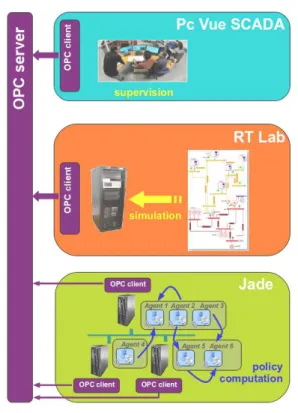
The platform includes various tools and sub-platforms interacting together
(Figure 1). The core of the platform is RT-Lab (Real-Time Digital Simulation
and Control LABoratory (Dufour et al., 2005): a distributed simulator that is
able to simulate, in real-time, dynamic models of any parts of a power grid. RT-Lab allows to test and design controllers for a large variety of devices includ-ing power converters, controllable generatinclud-ing units, renewable energy systems (wind turbin, photovoltaic panels). The interface with real equipments is possible through power amplifiers. The supervision of the network simulated with RT-LAb
Figure 1: Experimental platform
is based on PcVue which allows to collect data and visualizes the dynamics of the simulation.
The agents we used to control generating units are implemented using Jade
(Java Agent DEvelopment Framework) (Bellifemine et al., 2007). The
multi-agent system is hosted by several PC connected by an ethernet network. Each PC can host several agents. Jade eases communications between agents through a support for message-passing: agents hosted in same PC communicate through Java RMI, otherwise HTTP protocol is used.
Jade, RT-Lab and PCVue are able to interact thanks to an OPC5server. Each
of them used an OPC client to exchange data. For Jade, each agent used its own
OPC client with respect to distribution and decentralization properties (Figure1).
6.2. Experimental Network
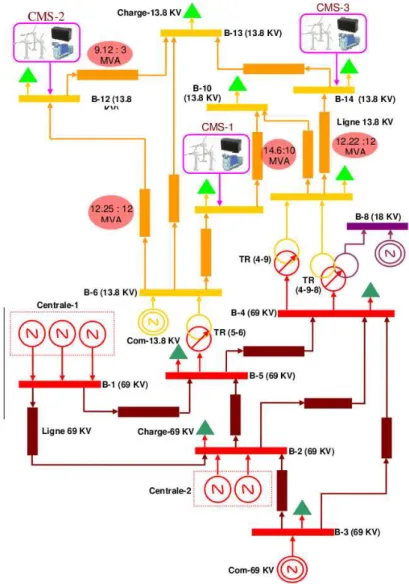
Figure 2: Test network
For our experiments, we use an IEEE 14 nodes network slightly modified as
depicted in Figure2. Several virtual power plants have been added whose
control-lable generating units are diesel power generators (named CMS in the figure2).
Each of them is able to generate profiles pithat range from 10% to 95% of pimax,
(C1) : 0.10 ∗ p
imax ≤pi ≤0.95 ∗ p
imax.
In addition, the fuel consumption of each generating unit is quadratic. It is worth noticing that the units with the biggest production capacity are also the units with
the highest cost. Finally, parameters tup, tdnand tcl are operational time limits (in
minutes) corresponding respectively to the minimum up time, the minimum down time and the cold start time. For each scenario, we consider the demand over twenty-four hours.
pmax fuel consumption depending of the output profile pi tup tdn tcl
10.8 KW 5.13pi 2−10 .19pi+ 29.53 80 80 80 6.30 KW 5.00pi 2−10 .00pi+ 29.72 80 80 80 5.40 KW 4.94pi 2−9 .92pi+ 29.79 80 80 80
Table 2: Diesel power generators features
It is worth noticing that the main source of uncertainty in this network is the unpredictable breakdowns of diesel power generators. To address this aspect, we add all possible breakdowns situations as part of the observations the agents can receive. Specifically, we use a Poisson distribution to describe the probability that a breakdown occurs for each generator unit over periods of time, independently from the other generator units.
The fuel consumption functions (Table2) are of crucial importance in
compet-itive settings. For instance, under the assumption of rational agents, this informa-tion can be used to predict the schedules of the other agents, which is undesirable in a competitive setting. Hence, we would like this information to be preserved during information exchange between agents. This highlights the necessity for a distributed algorithm that can preserve private information of each agent.
Each agent in charge of a diesel power generator starts its life cycle by reg-istering on the Jade platform. In this way, its name and IP address are stored by a Directory Facilitator agent, which is in charge of the ’Yellow pages’ phone book. Then, agents can communicate with one another through messages. Once all agents are registered, they all receive at a DSUC instance corresponding to one specific scenario from a human operator interacting with the RT-Lab platform. 6.3. Experimental Results
This subsection presents the experimental results obtained for different sce-narios. We distinguish between four scenarios along with the associated DSUCs.
The first set of experiments (Scenario 1) is our baseline since it assumes no unpre-dictable event (e.g., breakdowns) can occur at the execution phase. The second set of experiments (Scenario 2) extends Scenario 1 and allows unpredictable break-downs to occur. These experiments highlight the necessity of representing unit commitment problems using DSUCs. The third set of experiments (Scenario 3) compares performances we obtain using a reactive approach i.e., considering a planning horizon T = 1 ( this approach is referred to as P-DPGO-one-stage) ver-sus an approach that takes into account long term effects of present decisions, i.e., the P-DPGO algorithm. The last set of experiments (Scenario 4) provides the op-portunity to evaluate the scalability of the P-DPGO algorithm as the number of agents increases.
Demand profiles we use for each of these scenarios is depicted in Figure3. For
each scenario, we run the P-DPGO algorithm, simulated the resulting policies and reported: (a) the number of units involved; (b) load profiles for all units involved; (c) breakdown events when they occur. In Scenarios 3 and 2, we also reported the cumulated cost over the planning horizon each experimented approach yields. In Scenario 4, we reported the total time required to find a solution using the P-DPGO algorithm as the number of agents increases.
!" #!!!" $!!!!" $#!!!" %!!!!" %#!!!" &!!!!" &#!!!" '!!!!"
$" %" &" '" #" (" )" *" +" $!" $$" $%" $&" $'" $#" $(" $)" $*" $+" %!" %$" %%" %&" %'"
!"#$%&'(#)& *+,$&'-".%/)& ,-./01"23456-"$" 789-0/3:4"&;" ,-./01"23456-"&" 789-0/3:4"$<"%;" ,-./01"23456-"%" 789-0/3:4"&;"
Figure 3: Demand of power
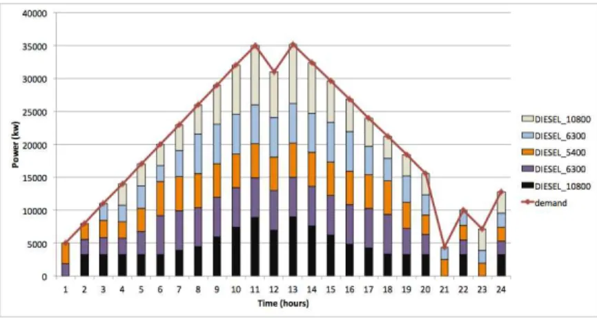
Scenario 1. In this scenario, we consider two configurations with five and six
diesel power generators, respectively. We simulate policies the P-DPGO algo-rithm pre-computed in face of different demand profiles over 24 hours. For the
two configurations, Figure 4 and Figure 5 reported traces of these simulations. Cumulative histrograms allow to easily visualize the commitment of each unit .
Clearly, other all tested instances (as demonstrated by Figure 4 and Figure 5),
P-DPGO always produces policies that can meet the demand in the absence of unpredictable events. !" #!!!" $!!!!" $#!!!" %!!!!" %#!!!" &!!!!" &#!!!" '!!!!"
$" %" &" '" #" (" )" *" +" $!" $$" $%" $&" $'" $#" $(" $)" $*" $+" %!" %$" %%" %&" %'"
!"#$%&'(#)& *+,$&'-".%/)& ,-./.01$!*!!" ,-./.01(&!!" ,-./.01#'!!" ,-./.01(&!!" ,-./.01$!*!!" 234562"
Figure 4: Scenario 1: DSUC with 5 units
!" #!!!" $!!!!" $#!!!" %!!!!" %#!!!" &!!!!" &#!!!" '!!!!"
$" %" &" '" #" (" )" *" +" $!" $$" $%" $&" $'" $#" $(" $)" $*" $+" %!" %$" %%" %&" %'"
!"#$%&'(#)& *+,$&'-".%/)& ,-./.01#'!!" ,-./.01$!*!!" ,-./.01(&!!" ,-./.01#'!!" ,-./.01(&!!" ,-./.01$!*!!" 234562"
Figure 5: Scenario 1: DSUC with 6 units
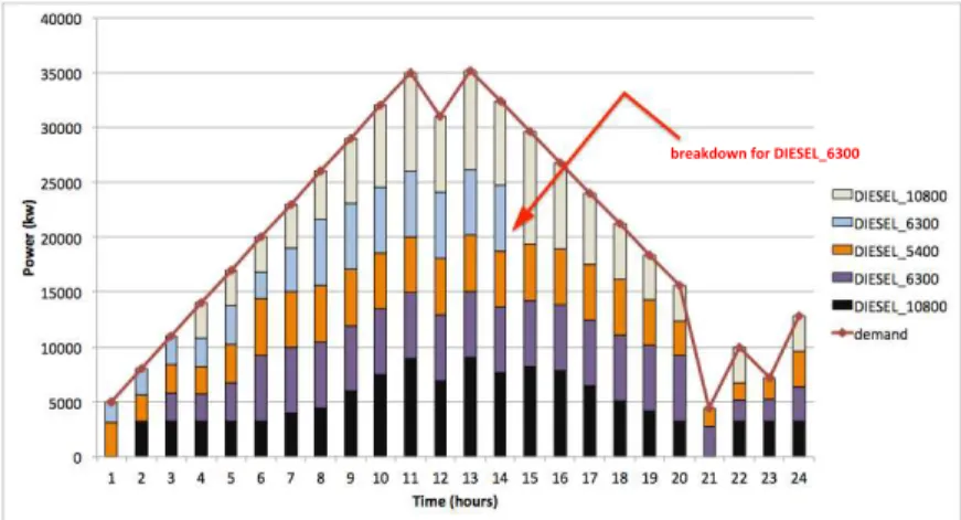
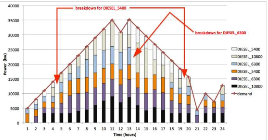
Scenario2. Here, we extend Scenario 1 and simulate unpredictable breakdowns
of the diesel power generators. It is in such a setting that P-DPGO fully demon-strates its advantage over classical (centralized) approaches. It produces (in a
distributed manner) policies that can take into account events that may occur at
the execution phase, e.g., unpredictable breakdowns as illustrated in Figure6and
Figure7. Specifically, Figure 6 shows that P-DPGO produces policies that can
automatically switch to situations where one unit (here unit ‘DIESEL 6300’) is no longer available for the remaining of the planning horizon while still meeting
the demand. Figure7presents another extreme case where many units (here units
‘DIESEL 5400’ and ‘DIESEL 6300’) experienced breakdowns at different period in the planning horizon. Yet, P-DPGO preserves ability to meet the demand based
on the remaining units. Non surprisingly, Figure 8shows that these breakdowns
can significantly affect the total costs of P-DPGO policies. Specifically, when as-suming unpredictable events can occur, the total cost of P-DPGO policies is about
2,5 per cent of than the case where we assume no unpredictable events can occur.
!" #!!!" $!!!!" $#!!!" %!!!!" %#!!!" &!!!!" &#!!!" '!!!!"
$" %" &" '" #" (" )" *" +" $!" $$" $%" $&" $'" $#" $(" $)" $*" $+" %!" %$" %%" %&" %'"
!"#$%&'(#)& *+,$&'-".%/)& ,-./.01$!*!!" ,-./.01(&!!" ,-./.01#'!!" ,-./.01(&!!" ,-./.01$!*!!" 234562" 0%$1(2"#3&4"%&567879:;<==&
Figure 6: Scenario 2 with 5 units and one breakdown occuring
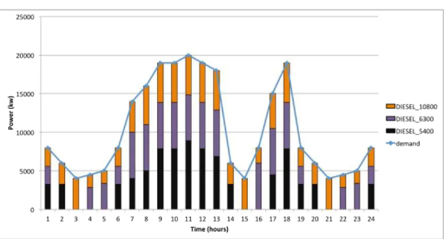
Scenario 3. This scenario compares the performances of P-DPGO-one-stage and
P-DPGO algorithms. P-DPGO-one-stage refers to the use of P-DPGO with a plan-ning horizon T = 1, in other words without taking into account long term effects of present decisions. To compare P-DPGO-one-stage and P-DPGO performances,
we consider three diesel power generator units. Figure9and Figure10report
de-mand and production profiles over 24 hours for P-DPGO and P-DPGO-one-stage algorithms, respectively. For this specific configuration, both approaches meet the
demand over the entire planning horizon. However, Figure11offers the
opportu-nity to compare the qualitative performances of each approach with respect to the total costs they induce. In particular, we note that P-DPGO-one-stage requires a
!" #!!!" $!!!!" $#!!!" %!!!!" %#!!!" &!!!!" &#!!!" '!!!!"
$" %" &" '" #" (" )" *" +" $!" $$" $%" $&" $'" $#" $(" $)" $*" $+" %!" %$" %%" %&" %'"
!"#$%&&'(#)& *+,$&'-".%/)& ,-./.01#'!!" ,-./.01$!*!!" ,-./.01(&!!" ,-./.01#'!!" ,-./.01(&!!" ,-./.01$!*!!" 234562" 0%$1(2"#3&4"%&567879:;<==& 0%$1(2"#3&4"%&567879:>?==&
Figure 7: Scenario 2 with 6 units and 3 breakdowns occuring
!" #!!!" $!!!" %!!!" &!!!" '!!!" (!!!" )!!!" !" '" #!" #'" $!" $'" !" #$ %&' (% )*+,%&-"./#(% *+,-" *+,-"./-0"123456+.7,"
Figure 8: Cumulated cost for Scenario 2 with three breakdowns
total cost that is 7 per of cent higher than that from P-DPGO. Clearly, the advan-tage of the P-DPGO algorithm comes from its ability to anticipate future effects
of present choices, whereas P-DPGO-one-stage cannot. For example, in figures9
and10, we observe that P-DPGO allow to turn off the ‘DIESEL 10800’ (the unit
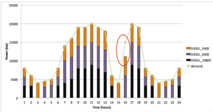
with the highest cost) more often than with P-DPGO-one-stage. In addition there are many cases in which P-DPGO-one-stage fails to meet the demand as it cannot take into account future effects of present decisions. To illustrate this point, we slightly modify the demand previously used: at time t = 16 we increase the
de-!" #!!!" $!!!!" $#!!!" %!!!!" %#!!!"
$" %" &" '" #" (" )" *" +" $!" $$" $%" $&" $'" $#" $(" $)" $*" $+" %!" %$" %%" %&" %'"
!"#$%&'(#)& *+,$&'-".%/)& ,-./.01$!*!!" ,-./.01(&!!" ,-./.01#'!!" 234562"
Figure 9: Scenario 3: DSUC with 3 units solved with P-DPGO
!" #!!!" $!!!!" $#!!!" %!!!!" %#!!!"
$" %" &" '" #" (" )" *" +" $!" $$" $%" $&" $'" $#" $(" $)" $*" $+" %!" %$" %%" %&" %'"
!"#$%&'(#)& *+,$&'-".%/)& ,-./.01$!*!!" ,-./.01(&!!" ,-./.01#'!!" 234562"
Figure 10: Scenario 3: DSUC with 3 units solved with P-DPGO-one-stage
mand from 8000 to 15000 and at time t = 17 from 15000 to 20000 (demand profile
2 on figure3). In this new case, P-DPGO-one-stage fails to satisfy the load
de-mand. Indeed, at time t = 15 , P-DPGO-one-stage turns off the ‘DIESEL 10800’
as illustrated in Figure13. Due to the operation time limit of the unit (Table2),
unit ‘DIESEL 10800’ cannot be restarted and fails to meet the load demand at t = 16. In contrary, the P-DPGO algorithm uses a long term planning, hence it
can handle this new case (Figure12).
Scenario 4.. The complexity of DSUCs increases linearly with the planning
!" #!!" $!!!" $#!!" %!!!" %#!!" &!!!" &#!!" '!!!"
$" %" &" '" #" (" )" *" +" $!" $$" $%" $&" $'" $#" $(" $)" $*" $+" %!" %$" %%" %&" %'"
!" # "$ %& '( )* +, &)-./ ) 01#')-2+"3,/) ,-./."01/2"3453674-894./:;9" ,-./."01/2"345367":<;-=1/2>"
Figure 11: Scenario 3: DSUC cumulated cost difference between DPGO-one-stage and P-DPGO !" #!!!" $!!!!" $#!!!" %!!!!" %#!!!"
$" %" &" '" #" (" )" *" +" $!" $$" $%" $&" $'" $#" $(" $)" $*" $+" %!" %$" %%" %&" %'"
!"#$%&'(#)& *+,$&'-".%/)& ,-./.01$!*!!" ,-./.01(&!!" ,-./.01#'!!" 234562"
Figure 12: Scenario 3: DSUC with 3 units solved with P-DPGO
demonstrating the scalability of the P-DPGO algorithm, we run experiments for increasing the number of units. To this end, over each tested configuration, we keep track of both the number of messages agents exchanged during the plan-ning phase, and the computational time required in order to find the final solution. Overall, both the computational time and the number of messages grow expo-nentially with increasing number of units. For instance, the number exchanged messages we recorded is about 85 thousands for three units and up to 5 millions for six units. Similar results hold for the computation time as the number of units
!" #!!!" $!!!!" $#!!!" %!!!!" %#!!!"
$" %" &" '" #" (" )" *" +" $!" $$" $%" $&" $'" $#" $(" $)" $*" $+" %!" %$" %%" %&" %'"
!"#$%&'(#)& *+,$&'-".%/)& ,-./.01#'!!" ,-./.01(&!!" ,-./.01$!*!!" 234562"
Figure 13: Scenario 3: DSUC with 3 units solved with P-DPGO-one-stage
increases. 0.001 0.01 0.1 1 10 100 1000 10000 1 2 3 4 5 6 7 8 9 10
Time in seconds (logscale)
Number of units
Figure 14: Time computing with different DSUC size
7. Conclusion
This paper explores the economic dispatch and unit commitment (UC) prob-lem which consists in finding the optimal schedules and amounts of power to be generated by a set of distributed units in response to an electricity demand. The motivation of this work is to propose a distributed approach to solve UC
prob-lems taking into account uncertainty from both demand and supply and privacy-preserving constraints.
We introduce an algorithmic framework that extends both stochastic and dis-tributed approaches to UCs in order to ensure electrical utilities do not explicitly communicate private information during the planning phase. We show how to recast distributed stochastic unit commitment problem into linearly constrained quadratic programs. The main contribution of the paper concern an offline and multi-agent distributed planning algorithm (termed P-DPGO) which combines a projected gradient descent and a communication protocol that allow electrical utilities to collectively find an optimal schedule strategy while ensuring private information remain unshared.
The performance of P-DPGO is evaluated over different stochastic scenarios using a real-time experimental platform. The experiments highlight the salient features of P-DPGO: it preserves private information, it takes into account long term decision effects and it handle uncertainty un supply and demand.
In the future, we plan to explore applying this approach to competitive scenar-ios, with self-interested agents. Furthermore, we will investigate P-DPGO theo-retical guarantees that can ensure we end with an optimal policy.
References
Aoki, K., Itoh, M., Satoh, T., Nara, K., Kanezashi, M., aug 1989. Optimal long-term unit commitment in large scale systems including fuel constrained thermal and pumped-storage hydro. IEEE Transactions on Power Systems 4 (3), 1065– 1073.
Bellifemine, F., Caire, G., Greenwood, D., 2007. Developing multi-agent systems with JADE. John Wiley and Sons.
Borghetti, A., Frangioni, A., Lacalandra, F., Lodi, A., Martello, S., Nucci, C., Trebbi, A., 2001. Lagrangian relaxation and tabu search approaches for the unit commitment problem. In: Power Tech Proceedings, 2001 IEEE Porto. Vol. 3. Bouffard, F., Galiana, F., Conejo, A., 2005. Market-clearing with stochastic
security-part i: formulation. Power Systems, IEEE Transactions on 20 (4), 1818–1826.
Boyd, S., Vandenberghe, L., 2004. Convex Optimization. Cambridge University Press.
Cohen, A., Yoshimura, M., feb 1983. A branch-and-bound algorithm for unit com-mitment. IEEE Transactions on Power Apparatus and Systems PAS-102 (2), 444–451.
Dechter, R., 2003. Constraint optimization. In: Constraint Processing. Morgan Kaufmann, San Francisco, pp. 363 – 397.
Dufour, C., Abourida, S., Belanger, J., nov 2005. Hardware-in-the-loop simula-tion of power drives with rt-lab. In: Proceedings of the 6th Internasimula-tional IEEE Conference on Power Electronics and Drives Systems, PEDS 2005. Vol. 2. pp. 1646–1651.
Fisher, M., dec 2004. The lagrangian relaxation method for solving integer pro-gramming problems. Management Science 50, 1861–1871.
Guan, X., Zhai, Q., Papalexopoulos, A., july 2003. Optimization based meth-ods for unit commitment: Lagrangian relaxation versus general mixed integer programming. In: Power Engineering Society General Meeting, 2003, IEEE. Vol. 2.
Kim, B., Baldick, R., may 1997. Coarse-grained distributed optimal power flow. IEEE Transactions on Power Systems 12 (2), 932–939.
Kok, J., Scheepers, M., Kamphuis, I., 2010. Intelligent Infrastructures, in the se-ries Intelligent Systems, Control and Automation: Science and Engineering. Springer, Ch. Intelligence in electricity networks for embedding renewables and distributed generation, pp. 179–209.
Kumar, A., Faltings, B., Adrian, P., 2009. Distributed constraint optimization with structured resource constraints. In: Proceedings of the 8th International Confer-ence on Autonomous Agents and Multiagent Systems, AAMAS 2009. Vol. 2. pp. 923–930.
Lesser, V., Tambe, M., Ortiz, C. L. (Eds.), 2003. Distributed Sensor Networks: A Multiagent Perspective. Kluwer Academic Publishers, Norwell, MA, USA. Mathews, G., Durrant-Whyte, H., Prokopenko, M., mar 2009. Decentralised
deci-sion making in heterogeneous teams using anonymous optimisation. Robotics and Autonomous Systems 57 (3), 310–320.