V
ALUATIONOFANOILFIELDUSINGREALOPTIONSANDTHEINFORMATION PROVIDED BYTERM STRUCTURESOFCOMMODITYPRICESLAUTIER Delphine
CEREG (University Paris IX) & CERNA (ENSMP) Email : [email protected]
Tel: 33 1 40 51 92 25
Address : CEREG
Université Paris IX Dauphine
75 775 Parix Cedex 16 France
V
ALUATIONOFANOILFIELDUSINGREALOPTIONSANDTHEINFORMATION PROVIDED BYTERM STRUCTURESOFCOMMODITYPRICESABSTRACT: This article emphasises that the information provided by term structures of commodity prices has an influence on the real option value and on the investment decision. We exhibit first of all the analysis framework: the evaluation of an oil field. We suppose that a single source of uncertainty -the crude oil price - affects -the investment decision. We also present -the two term structure models used to represent the dynamic behaviour of this price and to evaluate the net cash flows of the field. Then we present the real options valuation method. Lastly, simulations illustrate the sensibility of the real options to the term structure of commodity prices, and we analyse the investment signals given by the optional method. Our principal conclusions are twofold. Firstly, it is essential to take into account the information provided by the term structure of futures prices to understand the behaviour of the real option. Secondly, the investment signal associated with the optional method does not differ, for some specific price curves, from the one given by the net present value.
KEY WORDS: convenience yield stochastic models real option to delay crude oil term structure net present value.
S
ECTION1. I
NTRODUCTIONThe objective of this article is to highlight the impact of term structure of futures prices on real options value. The real option theory is based on an analogy with the financial options1. It aims to identify the optional component included in most investment projects, and to evaluate it, when possible. Its main advantage is that, contrary to the methods traditionally used for the selection of investment projects - like the net present value - it takes into account the flexibility of a project.
The theory leads to the identification of different families of real options and underlines that most investment projects include several options. However, in this article, even if the possession of an oil field implies the holding of several options, we only take into consideration the option to delay the exploitation until some useful information arrives and gives the signal to invest. We also suppose that a single source of uncertainty affects the project value: the crude oil price. As a consequence, the information given by this price has a crucial influence on the investment decision.
This price can be represented by a futures price, which is, at a specific date and conditionally on the information available at that date, an expectation of the future spot price. The term structure of commodity prices connects all the futures prices for different maturities. This curve can take different shapes. When the spot price is higher than the futures prices, there is backwardation. Given this information, a decrease in the future spot prices is expected. When conversely the spot price is inferior to the futures prices, the term structure is in contango, which means that one can wait for an increase in the future spot prices. Naturally, there are also more complicated prices curves, with for example a backwardation on the nearest maturities and a contango for long-term contracts.
With a term structure model, it is possible to compute a futures price for any expiration date, even if it is very far away. Thus, such a model enables the valuation of the net cash flows associated with the investment project and it gives all the information needed for the investment decision. Provided that we take into account this information, it is possible to understand the behaviour of the real option, which becomes consistent with the behaviour of a financial option.
This paper proceeds as follows. Section 2 is devoted to the analysis framework: we give some precision on the oil field characteristics and on the method used to represent the behaviour of the crude oil price. We also explain why we concentrate on the option to delay and we present this option. Section 3 introduces the optional method. The latter relies on two term structure models of commodity prices, which are presented. Section 4 analyses the sensibility of the real option to its main determinants. Section 5 is centred on the investment decision and shows that for certain term structures, the optional method does not differ from the net present value. Section 6 concludes.
1 A presentation of the real options theory can be find in Copeland et Antikarov (2001), Grinblatt et Titman (2001), Lautier
S
ECTION2. T
HEANALYSISFRAMEWORKThe analysis framework presents two characteristics. Firstly, we retain only the option to delay the exploitation. Secondly, we only consider the uncertainty associated with the crude oil price. Before we tackle the valuation itself, we shall justify these two choices.
2.1. A single real option
In this study, we only consider the option to delay the development of an oil field. Yet the real option theory shows that most of the time, an investment project includes more than one real option. The real options the most frequently evoked in the literature are the option to delay, the option to abandon, the time to build option, the option to alter operating scale, the option to switch use, the growth option, and the multiple interactive options. At least four of them are associated with the holding of an oil field. Among them, the option to delay is undoubtedly the simplest. It represents the possibility, for the owner of the field, to wait before investing, until some useful information arises. Naturally, the investor has other potentialities. Once the production has begun, it is for example always conceivable to renounce the project: this is the option to abandon. Likewise, the exploitation necessitates several successive investment steps: exploration, oil development, and production itself. Each step ameliorates the information on the level and the quality of the resource, and can lead to pursuit investment when the information is favourable or conversely to give up: this is the time to build option. Finally, it is possible to reduce or even to temporarily shut down the exploitation: this depicts the option to alter operating scale.
In view of this profusion, one may consider that it is simplistic to focus on a single real option. To explain this choice, we argue that the valuation of real options, which follows the methods developed for the financial assets, presents some difficulties arising from the differences between real and financial assets2. However, the aim of this article is not to deal with these difficulties but to study the relationship between real options and the information given by term structure of price. Therefore, the most elementary set up was retained: the case of a single option.
Among the different options included in the project, we choose the option to delay. Several reasons justify this choice. Firstly, it is quite simple to evaluate. Secondly, amid the different steps of the project, the development phase necessitates the most important expenditures. Therefore, the option to delay is probably the most expensive one. Thirdly, we did not take into account the possibility to shut down temporarily the exploitation because this kind of operation is very harmful for the underground mines and for the oil fields. The interruption of the exploitation causes indeed the flood of the mines. And the reopening cost is not very far from the cost of a new development. Fourthly, the
2The latter are divisible, fungible, and most of the time actively traded on a secondary exchange. This is not the case for the
option to abandon is neglected because, once the exploitation has begun in the petroleum industry, it is generally conducted until the end.
2.2. The real option to delay
The option to delay is the simplest real option and undoubtedly the most frequently evoked in the literature3. It represents the possibility to wait before investing in order to collect some useful information.
To present the real option to delay, let us establish an analogy between the holding of a call on a share and the possession of exploitation rights on a field. The first makes it possible to buy a share and to enjoy the dividends and the capital gain or loss. The second gives the possibility to exploit the field and to benefit from the net present value of the resource. Because an oil field can be difficult to sale, or to shut down temporarily, such an investment is regarded as irreversible. This real option is American, because the investor has the choice to develop whenever he wants, until his rights expire.
The analogy between a financial call and the real option to delay presents nevertheless two limits. First of all, the real option expiration date can be very far away4. Secondly, the exercise of the
financial call gives rise to the immediate transfer of the property rights on the underlying asset. This is not the case when the real option is exercised. Indeed, when the field is exploited, one must wait several weeks or months until the crude oil arrives to the consumption areas. These differences have an influence on the real option valuation.
2.3. A single source of uncertainty
Last particularity of this study: we suppose that the crude oil price is the only source of uncertainty having an impact on the investment value. Such a choice implies that we made several assumptions: the reserves, the extraction costs and the development costs are supposed to be known; we ignore the expropriation risk; technological progress is neglected, and the volume of the reserves and their production costs are independent of the exploitation date.
The choice of this framework can be explained as follows. During a long time, in this industry, the most important question concerning a field’s exploitation was: how can we develop at the lower cost? Today, most of the time, the newly discovered fields are not immediately exploited. One waits for a higher price, especially when the reserves are substantial. Lastly, in our example, the uncertainty is a purely exogenous factor, on which the operator has no power. This choice amounts to saying that the investor has no possibility to influence the crude oil price. Such an assumption is not innocuous for most operators in the crude oil market.
3 This real option was also studied by McDonald and Siegel (1986), and Brennan et Schwartz (1985).
4 The length of the exploitation rights on a petroleum field is extremely variable: it can stretch over 99 years or it can be less
Thus, uncertainty is only due to the crude oil price. Because only the price has an impact on the project’s value and on the investment decision, we pay a special attention to the representation of the price dynamic. Indeed, in order to appreciate the value of the option to delay the exploitation, the value of its underlying asset must be known. Yet the later depends directly on the hypothesis concerning the evolution of the crude oil price. In this situation, the term structure models of commodity prices can be useful tools. We first of all present the two models used. Then we analyse the impact of each model on the project’s net present value.
2.3.1. The two term structure models of commodity prices
We use two well-known models: Brennan and Schwartz developed the first in 1985, and Schwartz proposed the second in 1997. The principal difference between these two models is due to their representation of the prices dynamic behaviour. Brennan and Schwartz choose a geometric Brownian motion for the spot price. However, a few years later, Schwartz renounced to this modelling and referred to a mean reverting behaviour.
Brennan and Schwartz’s model
Brennan and Schwartz’s model is the first and the simplest version of a term structure model of commodity prices. In this model, the movements of the futures prices depend only on the spot price. The dynamic of the latter is the following:
dz t S dt t S t dS( ) ( ) S ( ) where: - S is the spot price,
- µ is the drift,
- is the spot price’s volatility,S
- dz is an increment to a standard Brownian motion associated with S.
This formulation means that the spot price’s variation at t is independent of the previous variations, and the drift µ conducts the prices evolution. The uncertainty affecting the price’s evolution is proportional to the level of S: when inventories are rare, the spot price is high; in this situation, any modification in the demand has an important impact on the spot prices, because the physical stocks are not sufficiently abundant to absorb the prices fluctuations.
The solution of the model, for a futures price having an expiration date T, is5:
F S t T( , , ) Se(r c )
where: - r is the risk free interest rate, assumed constant, - c is the convenience yield, assumed constant, - is the contract’s maturity: = T - t
Briefly defined, the convenience yield represents the comfort associated with the holding of inventories. Its correlation with the spot price is positive.
Schwartz’s model
5 The solution of the models can be obtained using a Feynman-Kac solution. For more details, see for example Lautier
In Brennan and Schwartz’s model, the spot price dynamic ignores that the operators in the physical market adjust their inventories to the evolution of the spot price, and to changes in supply and demand. Moreover, this representation ignores that a futures price does not depend only on the spot price, but also on the convenience yield. The latter is a parameter and it is supposed to be constant. However, in 1989, Gibson and Schwartz showed that such an analysis is limited. They proposed to introduce the convenience yield as a second state variable, the latter having a mean reverting behaviour. Schwartz’s model includes these recommendations and retains the following dynamic:
)
(
)
(
)
(
)
(
)
(
)
(
C
C
S
S
dz
dt
t
C
t
dC
dz
t
S
dt
t
S
t
C
t
dS
with : , S, C > 0 where : - S is the spot price,- C is the convenience yield, - µ is the drift of the spot price,
- is the long run mean of the convenience yield, - is the speed of adjustment of C towards - Sis the spot price’s volatility,
- C is the volatility of the convenience yield,
- dzS is an increment to a standard Brownian motion associated with S, - dzC is an increment to a standard Brownian motion associated with C. The spot price and the convenience yield follow a joint diffusion process:
dt = Et[dzSdzC]
where is the correlation coefficient linking the two Brownian motions.
This representation of the convenience yield behaviour supposes that there is an average level of physical stocks, which satisfies the needs of the industry. Therefore, the operators behave such as the volume of stocks and consequently the convenience yield converge on this level. When the convenience yield is low, stocks are abundant and the operators sustain a high storage cost compared with the benefits associated with the holding of the merchandise. If they behave rationally, they will try to eliminate the surplus stocks. Conversely, when the convenience yield is high they will tend to reconstitute their stocks.
The solution of Schwartz’s model is the following: HC B e S T t C S F( , , , ) with : H
1e
/ , ,
2 32 2 2 2 21
1
4
1
2
1
r
e
e
B
C C S C C S C
This model is more realistic than the previous one. It authorizes price curves that are more varied and closer to the curves observed on commodities markets. However, this model is also more complex. Particularly, it includes seven parameters whereas the previous has only two of them. 2.3.2. The representation of the prices dynamic and its influence on the net present value.
In order to show how the representation of the spot price’s behaviour influences the value of the net future cash flows, we study the sensitivity of the net present value. We make an additional hypothesis for the calculation of the NPV: we suppose that the exploitation leads to the production of one single crude oil barrel at the end of each year during a period of N years.
The NPV is:
N T N T p B aT I C T a PV NPV 1 0 1 ) , ( ) , (where : - PV(a,T) is the net present value of a barrel produced in T, a is the discount rate,
Cp is the cost of production per barrel. It is supposed to be constant during the project’s life. B(a,T) is the present value of one dollar (equal to e-aT if a is constant),
I0 is the initial investment.
We made three assumptions concerning the crude oil price behaviour. The first one relies on the practice commonly adopted in the petroleum industry. It consists in supposing that the price will be constant during the whole life of the project. The two others hypotheses are based on the term structure models previously presented.
Each assumption leads to a different net present value. When the Brennan and Schwartz’s model is retained, it becomes:
N T N T rT P cT C e I S e S T t S NPV 1 1 2 1 0 ) , , ( with :
N T cT e 1 1 and 0 1 2 C e I N T rT p
When Schwartz’s model is used, the net present value is:
N T N T rT P t HC C e I S e T A t S T t C S NPV 1 1 2 1 0 ) ( ) ( ) ( ) , , , ( with:
4 5 . 0 ² [ ) ( exp ) ( 2 2 2 2 H H A C S C C ,
N T t HC e T A 1 ) ( 1 ( ) , and 0 1 2 C e I N T rT p
Unless clearly specified, the data retained for the calculations presented below are the following: the project lifetime N is fixed at 15 years. The production cost CP is established at 7 dollars per barrel. This level is realistic for an exploitation in the North Sea. In order to determine I0, we
considered that a project is profitable when its net present value is annulled for a constant spot price of 12 dollars per barrel and for a discount rate of 15%. Hence, I0 was fixed at 25 dollars. These values can be discussed. The interest of the exercise is not to work with values corresponding to a specific project, but to compare the valuation methods.
In order to compute the futures prices corresponding to each term structure model, one must also precise the parameters and the state variables parameters. These values are directly extracted from empirical tests previously performed on the crude oil market (Lautier and Galli, 2001). Therefore, the convenience yield is set to 0.2. Moreover, for Schwartz’s model, the parameters values are the following: the long run mean of the convenience yield, , is equal to 0.1; the spot price’s volatility S is set to 0.3, and the volatility of the convenience yield C is supposed to be 0.4. The speed of adjustment is established at 2, the correlation coefficient is fixed at 0.9 and the risk premium associated with the convenience yield is set to 0.1. Lastly, the NPV discount rate and the interest rate are supposed to be equal to 5%.
The study of the evolution of the NPV, computed with the three methods, leads to several conclusions. The first are valid whatever the hypothesis concerning the price behaviour. As is shown in Figures 1 and 2, the NPV is an increasing function of the initial crude oil price and of the project lifetime. However, it decreases with the exploitation cost, with the initial investment, and with the discount rate.
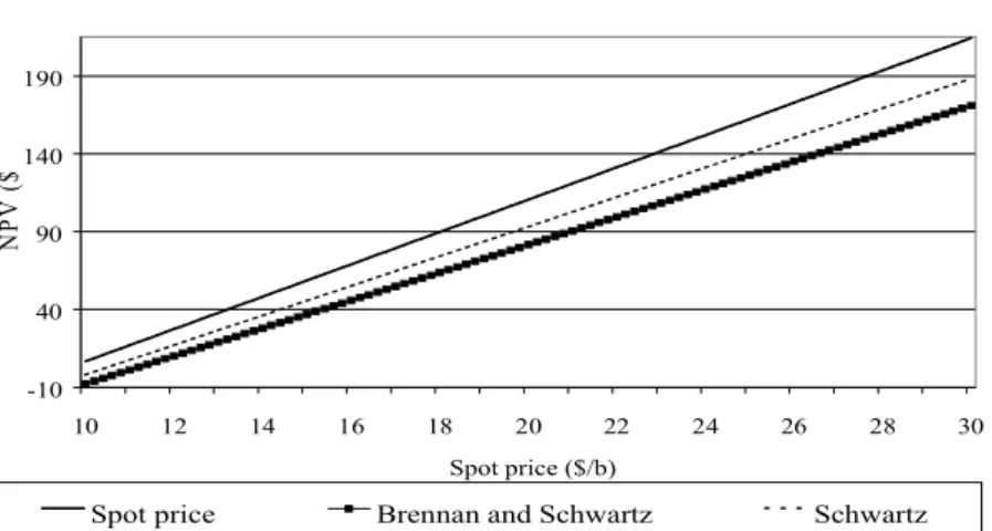
The relationship between the NPV and the initial spot price is linear and positive, whatever the method retained to compute the net cash flows associated with the project, as is shown in Figure 1.
Figure 1. Net present value as a function of the spot price
-10 40 90 140 190 10 12 14 16 18 20 22 24 26 28 30 Spot price ($/b) N P V ( $)
Spot price Brennan and Schwartz Schwartz
The study of the evolution of the project NPV as a function of its lifetime (Figure 2) shows that an increase in the project lifetime has a positive influence on the NPV. However, this influence diminishes as the expiration date rises.
As far as Brennan and Schwartz’s model is concerned, the relationship between the interest rate and the convenience yield fixes the shape of the entire term structure of prices, and it is essential for the NPV. For Schwartz’s model, the main determinants of the price curve, for the nearest expiration dates, are the initial level of the convenience yield, the speed of adjustment , and the long
run mean . When the speed of adjustment is high, all things being equal, the main parameter is the long run mean, because the convenience yield can not go very far from it. Conversely, when the speed of adjustment is low, the prices curve is strongly influenced by the initial distance between the convenience yield and the long run mean (Lautier, 2002).
Figure 2. Net present value as a function of the project lifetime
-20 0 20 40 60 80 100 120 1 5 10 15 20 25 30 35 Lifetime (years) N P V ( $)
Constant price Brennan and Schwartz Schwartz
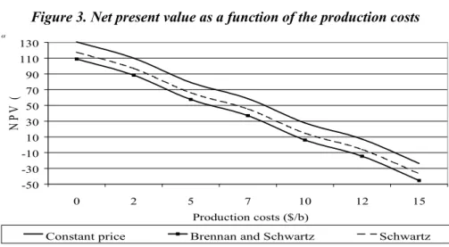
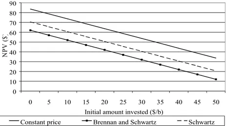
Figures 3, 4 and 5 illustrate that the net present value, whatever the hypothesis retained to represent the spot price evolution, is a decreasing function of the production costs, the initial amount invested, and the discount rate.
Figure 3. Net present value as a function of the production costs
-50 -30 -10 10 30 50 70 90 110 130 0 2 5 7 10 12 15 Production costs ($/b) N P V ( $)
Constant price Brennan and Schwartz Schwartz
0 10 20 30 40 50 60 70 80 90 0 5 10 15 20 25 30 35 40 45 50
Initial amount invested ($/b)
N
PV
(
$)
Constant price Brennan and Schwartz Schwartz
Figure 5. Net present value as a function of the discount rate
0 10 20 30 40 50 60 70 80 90 2% 4% 6% 8% 10% 12% 14% 16% 18% Discount rate N P V ( $)
Constant price Brennan and Schwartz Schwartz
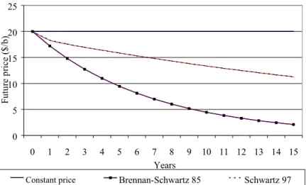
These simulations also show that in all the cases presented above, the NPV associated with Schwartz’s model is always the lowest. Then comes the one associated with Brennan and Schwartz’s model. Lastly, the NPV associated with the constant price hypothesis is systematically the highest. This result depends however on the parameter values, which correspond to a specific situation, illustrated by Figure 6: all the prices curves are in backwardation, especially for Brennan and Schwartz’s model.
0 5 10 15 20 25 0 1 2 3 4 5 6 7 8 9 10 11 12 13 14 15 Years Fu tu re p ri ce ( $/ b)
Constant price Brennan-Schwartz 85 Schwartz 97
Another set of parameters can lead to opposite conclusions. This is the case for the curves represented in Figure 7. In that situation, the term structure associated with Brennan and Schwartz’s model is in contango, and corresponds to the highest NPV: 76.05 dollars. The next highest NPV is the one associated with Schwartz’s model (71.32 dollars). The last is the one linked with the constant price assumption (70.18 dollars).
The valuation methods used to represent the dynamic behaviour of the crude oil price have therefore a strong influence on the project net present value. This will necessarily have an impact on the results of the optional method.
Figure 7. Term structures of prices, with S = 20$/b, r = 11%, and C = 0,07.
16 21 26 31 36 0 1 2 3 4 5 6 7 8 9 10 11 12 13 14 15 Years Fu tu re p ri ce ( $/ b)
Constant price Brennan-Schwartz 85 Schwartz 97
S
ECTION3. T
HEVALUATIONOFTHEREALOPTIONTODELAYThe real options valuation method is inspired by the one developed for the financial options. In this section, we present this method and we show how to apply it in our case.
A financial option is considered as an asset, whose price movements are totally specified by a set of underlying factors. The latter represent the sources of uncertainty influencing the price evolution of the derivative asset. For the simplest financial options, there is one single underlying factor: the price of the underlying asset. Therefore, the first step of an option valuation consists in determining the dynamic behaviour of the underlying asset price, in order to represent how the price will vary between the acquisition and the exercise date. Most of the time, this behaviour is characterised by two elements: a deterministic (the drift) and a random components.
The valuation method uses then arbitrage reasoning and leads to the construction of a hedge portfolio. Briefly speaking, the reasoning is the following: in a complete market where the transactions are continuous, a derivative asset can be duplicated by a combination of others existing assets. If the latter are sufficiently traded to be arbitrage-free evaluated, they can constitute a hedge portfolio whose behaviour replicates the derivative behaviour. Their proportions are fixed such as there are no arbitrage opportunities and the strategy is risk-free. Then, in equilibrium, the return of the portfolio must be the risk free rate. The valuation is made in a risk neutral world: it does not depend on the attitude toward risk of the operators.
3.2. The option to delay the exploitation and the term structure models
Two details must be added before we apply the valuation method to the real option to delay the oil field exploitation. First of all, in our example, the underlying factor is the crude oil price, whose behaviour is represented by a term structure model. Therefore, the choice of the model has an influence on the real option value. Secondly, in the case of the real option to delay, we do not estimate how long it is necessary to wait. We compute the critical exercise price of the option, namely the price corresponding to an option value above or equal to the project NPV.
3.2.1. The real option to delay associated with Brennan and Schwartz’s model
When we use Brennan and Schwartz’s model to represent the dynamic behaviour of the underlying asset, the real option to delay, V(S,t,T), satisfies the following equation:
0 ) ( 2 1 2 2 SS VSS r c SVS rV V The boundary condition of this equation is:
( , , ),0
max ) , , (S t T NPV S t T V This condition means that, at the expiration date T, if the NPV of the field is negative or equal to zero, the real option value is zero. If however the NPV is positive, the option value is equal to the NPV. This option is an American one: the investment can be undertaken at any moment.
Schwartz (1997) proposed an analytical solution to this equation. Supposing that the expiration date tends to the infinity, this solution is:
V S S
S
S
d
( ) *
*
1 2
with:
N T cT e 1 1 , 0 1 2 C e I N T rT p
, 2 2 2 2 2 2 1 2 1 S S S r c r c r d ,S
d
d
*
1 21
where S* is the critical price.Having an analytical solution is a huge advantage: the complexity and the slowness of the numerical methods used for Schwartz’s model, which are presented in the next paragraph, is a good illustration of that point. However, the analytical solution presents an important drawback: it can not be used when the convenience yield is negative or when it is equal to zero. Yet the convenience yield net of the storage costs can be negative when the market is in contango.
3.2.2. The real option associated with Schwartz’s model
In Schwartz’s model, the real option value, V(S,C,t,T), satisfies the differential equation :
0 ) ( 2 1 2 1 2 2 2 2 SS VSS CC VCC S CSVSC SVS r C VC C rV V The boundary condition is the same as the one presented before.This equation is more complex than the previous one, because Schwartz’s model supposes that two uncertainty sources have an impact of the real option: the spot price and the convenience yield. This equation does not have, to our knowledge, an analytical solution. Therefore, we used a finite difference method6: we replaced the partial derivatives by Taylor expansions. Among the various finite difference methods available, we chose the Crank-Nicholson method, for the stability of its solutions.
The discretization concerns the state variables S and C and the maturity = (T-t). The latter is divided into n time intervals of length k. The option value is recursively computed at the date (s-k), and it depends on its value in s, with t s T. When s = T, the option expires. The variation domain for S and C is divided into m intervals of length h. The grid is therefore constituted of the points (ih, jh, nk) in the space (S, C, t) such as7:
S = ih
for
0imC = jh for m/2 jm/2 t = nk for 0nnn
The option value is represented by a scheme in three dimensions: (i,j) (i,j)=U V ) V(ih,jh,nk V(S,C,t) n n .
6 This method is presented in the appendix. It is inspired by Bellalah (1990). Schwartz (1997) also used it.
7 The variation interval of the convenience yield differs from the one that was retained for the spot price: indeed the
Once the discretization has been completed, the Crank-Nicholson scheme centred in space is:
T V 2 W 2 X Y Z
U 1(i,j)
1 V 2 W 2 X Y Z
Un(i,j) C S C S C S n C S C S C S
with : R k i V S 4 2 2
R
h
k
W
C 2 24
hR k i X S C 8
R jh r ik Y 4
hR jh k Z 4
R rk T 2 2 2 2 rk R for 1im1 and (m/2)1 j(m/2)1An Alternative Directions Implicit (ADI) method is then applied on this scheme. This method is inspired by the one proposed by Mitchell and Mc Kee in 1970. It enables the resolution of the differential equation in two steps, despite the presence of a cross derivative. The use of an ADI method consists in introducing an intermediary term in order to separate, at each time step, the previous equations system into two sub-systems. Each of the latter is successively solved at each time step.
This numerical method, chosen for its rapidity, is still especially slow when it is applied in our context, for two reasons. First of all, the variation interval of the spot price is totally different of the one of the convenience yield. Secondly, the option expiration date is far away.
3.2. The difficulties of the real options valuation
The limits of the method used for the valuation of real options are twofold. Firstly, the valuation of financial options relies on hypotheses that are not really respected in the case of real assets. Secondly, the approach leading to the valuation is difficult to undertake.
The valuation of a financial option relies on assumptions concerning the market characteristics and the nature of the transactions. The market is supposed to be perfect, namely without transaction costs or taxes. Short sales are not restricted, and borrowing and lending rates are equal. All the assets are perfectly divisible, and the information concerning the prices and assets characteristics is freely available. The transactions are continuous. Therefore, it is always possible to modify the portfolios composition. The market is free of arbitrage opportunities.
The transposition of such a theoretical framework in the case of real options is not straightforward. It is indeed difficult to maintain that the perfect market hypothesis is still realistic. Firstly, in the world of real assets, markets imperfections can be considered as a necessary condition to the appearance and the exploitation of investment opportunities (Myers, 1977). Secondly, the real assets are sometimes not divisible.
Beyond these hypotheses, the valuation method of financial options must be cautiously used in the case of real options. The real assets are less traded than the financial assets. Thus, from the first step of the valuation, which consists in determining the most important uncertainty source affecting the real option price, some difficulties arise. The external valuation of the underlying asset guaranteed by the market, implicit in the case of financial options, can be impossible in a real assets world, when
the asset is specific, and has no value except for the firm holding it. In the most favourable situation, when there is a market for the real asset, it is probably narrow and imperfect, and the transaction will be characterised by uncompleted or asymmetrical information. Therefore, the second step of the valuation method, which supposes that the assets are traded with no arbitrage opportunities, must be cautiously undertaken. Particularly, the valuation will probably not be realised in a risk neutral world, or several risk neutral probabilities will coexist.
The limits of the valuation are therefore so important that the relevance of the analogy between real options and financial options becomes questionable. Does it mean that this analogy must be restricted to a purely qualitative analysis? The study of the determinants of the real options to delay, in section 4, gives an answer to that question.
S
ECTION4. S
ENSITIVITYOFTHEOPTIONVALUEThe simulations presented in this section are based on the term structure models of commodity prices presented previously. The models are used for the valuation of the net cash flows associated with the field, and for the computation of the real option value. The values of the parameters and the state variables are the same than those used in the first section, except for the project’s lifetime. The latter has been reduced to ten years, because of the slowness of the numerical method.
4.1. Real option, term structure of futures prices and state variables
The number of state variables changes with the term structure model. In Brennan and Schwartz’s model, only the spot price has an influence on the futures price evolution. In Schwartz’s model, the convenience yield is introduced.
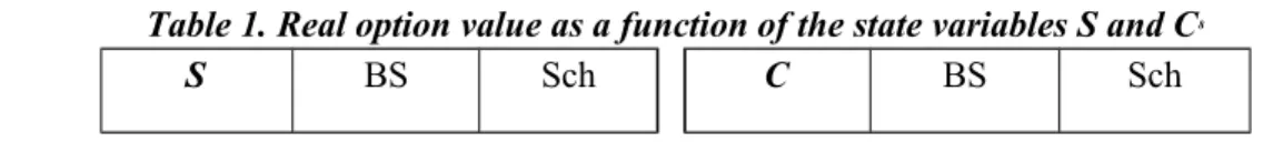
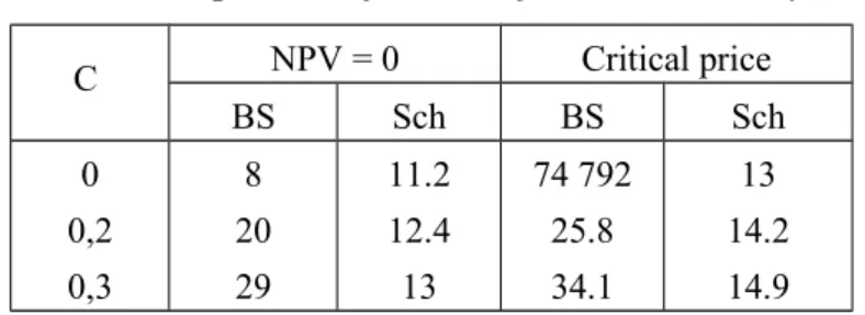
Table 1 reproduces the evolution of the value of the real option to delay the oil field exploitation when the spot price and the convenience yield vary. As far as the spot price is concerned, the conclusion is the same for the two models: the option’s value is an increasing function of this state variable. This result is consistent with the analogy between financial and real options previously made. Indeed in the two models, whatever the expiration date is considered, the futures prices is a positive function of the spot price. The latter affects the whole prices curve. Thus, a rise in the spot price conducts to an improvement of the project’s net present value, even if the prices curve is in backwardation. It just so happens that when the price of the underlying asset rises, we should observe an augmentation of the call value.
Table 1. Real option value as a function of the state variables S and C8
S BS Sch C BS Sch
14 18 22 1.34 4.24 10.63 10.52 35.58 60.74 0 0,2 0,3 179.8 4.24 0.18 47.27 35.58 30.14 S = 18 $/b ; C = 0.2 ;Cp =7$/b ; I0 = 25$ ; S =0.3 ; r = 5% ; = 0.1 ; = 2 ; C = 0.4 ; = 0.9 ; = 0.1 ;
The real option value is on the other hand a decreasing function of the convenience yield because in the two models, backwardation rises with the convenience yield, having thus a negative impact on the project net present value, and influencing therefore the value of the real option to delay.
The value of the real option associated with Schwartz’s model is finally a decreasing function of the speed of adjustment of the convenience yield, as is shown in Table 2.
Table 2. Option value as a function of the speed of adjustment
Sch 1 1.5 2 69.9 41.34 35.58 S = 18 $ ; C = 0.2 ; r = 5% = 0.1 ; S = 0.3 ; C = 0.4 ; = 0.9 ; = 0.1 ; CP = 7$, I0 = 25$
This result can be simply explained: the more the tendency of the convenience yield to return to its mean rises, the more the uncertainty associated with the long-term cash flows of the project diminishes. In this situation, the behaviour of the real option value is consistent with what would have been expected of a financial option: the option value increases when the volatility growths. And the more the speed of adjustment tends toward zero, the more the results obtained with the two-factor model are close to those issued from Brennan and Schwartz’s model.
4.2. Real option, term structure of futures prices and exploitation conditions
A second series of simulations analyses the impact of the exploitation conditions on the real option value. These conditions arise from the crude oil market itself (extraction cost per barrel and initial investment expenses) and more generally to the environment (level of interest rates).
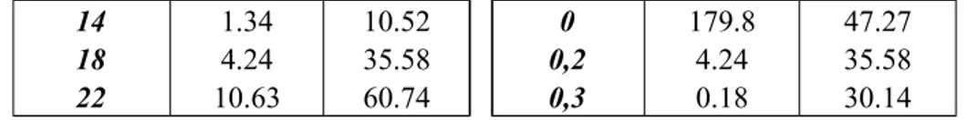
The study of the real option value establishes that it is a decreasing function of the extraction cost per barrel CP and the initial amount invested I0 (Table 3). It is also an increasing function of the interest rate (Table 4). These results are consistent with the behaviour of a financial option: the call value diminishes with the value of the underlying asset and the exercise price. However, it is a positive function of the interest rates.
Studying the way the production cost per barrel influences the option value authorizes firstly similar conclusions for the two models. When these costs rise, the option value diminishes. An increase in the production costs reduces indeed the net futures cash flows associated with the project and therefore the value of the underlying asset. This leads naturally to a decline of the call value. Likewise, when the production cost raises, the investment critical price increases: the price per barrel must ascend to compensate for the negative impact of the production cost on the cash flows. Secondly, the results depend on the model. The value of the real option associated with Brennan and Schwartz’s model is indeed lower than the one associated with Schwartz’s model, because backwardation is more
pronounced for the one-factor model. Consequently, the value of the underlying asset diminishes more rapidly.
Table 3. Real option value as a function of the exploitation conditions
CP ($/b) BS Sch I0 ($) BS Sch 5 7 10 9.22 4.24 1.69 50.94 35.58 13.04 20 25 30 5.36 4.24 3.4 40.58 35.58 30.59 S =18 $ ; I0 =25$ ;C=0.2 ; r = 5% ; = 0.1 ; = 2 ; S = 0.3 ; C = 0.4 ; = 0.9 ; = 0.1 ;When we study the impact of the initial amount invested (the option exercise price) we reach similar conclusions. The real option value decreases with the initial expenses.
Lastly, the study of the sensitivity to the interest rate shows that the more the interest rate is high, the more the real option value rises. The delay of exploitation leads indeed to the postponement of the initial expenses. The latter can be invested in the financial markets until the option is exercised and this investment is more interesting when the interest rate is high.
Table 4. Real option value as a function of the interest rate
r (%) BS Sch 3 5 7 2.85 4.24 5.94 29.73 35.58 40.7 S =18 $ ; Cp =7$/b ; I0 = 25$ ;C=0.2 ; = 0.1 ; = 2 ; S = 0.3 ; C = 0.4 ; = 0.9 ; = 0.1 ;
Comparing the two models leads however to the conclusion that Brennan and Schwartz’s model is more sensitive to the interest rate. When the interest rate rises from 3 to 5%, there is a 49% increase of the call value for the one-factor model whereas the variation is only of 19.7% for the two-factor model. This stronger sensitivity of the one-two-factor model appears also with the two other parameters, namely the exploitation costs and the initial expenses, but it manifests itself more intensively with the interest rate.
The study of the option sensitivity to its main determinants leads to two conclusions. Firstly, the real option to delay behaves like a financial call. Therefore, the analogy between real and financial options is relevant, not only qualitatively, but also quantitatively. Secondly, the real option value is sensible to the choice of a specific term structure model to evaluate the net future cash flows of the project. The net present value and the real option value depend strongly on the hypotheses retained concerning the dynamic of the crude oil price.
This section presents the results of simulations aiming to study the influence of the information provided by term structure of commodity prices on the investment decision. In order to determine when the investment must be undertaken, we retained two methods. The first is the NPV. In that case, the investment must be undertaken when the spot price is sufficiently high to lead to a null NPV. The second method is optional: it defines the price leading to the exercise of the real option. 5.1. The investment threshold and the level of the convenience yield
Table 5 shows how the investment threshold evolves when the convenience yield rises9. The results arouse three remarks.
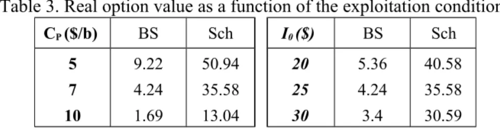
First of all, the figures obtained with the Brennan and Schwartz’s model, when the convenience yield tends toward zero10, are surprising. The critical price to invest, in that case, has no economical significance: 74 792 dollars per barrel! In that situation the net present value method which recommends an immediate investment must be preferred to the optional approach. The latter is of little interest because it is based on a term structure model which is not suited for distant maturity dates. Indeed, with this model, when the convenience yield is lower than the interest rate, the term structure of prices is in contango, and the futures prices can attain, for distant maturity dates, values having no economical sense.
Table 5. Critical price as a function of the convenience yield 11
C NPV = 0 Critical price BS Sch BS Sch 0 0,2 0,3 8 20 29 11.2 12.4 13 74 792 25.8 34.1 13 14.2 14.9 S = 18 $/b ; Cp =7$/b ; I0 = 25$ ; r = 5% ; = 0.1 ; = 2 ; S = 0.3 ; C = 0.4 ; = 0.9 ; = 0.1 ;
Secondly, when the convenience yield is higher than the interest rate (C = 0.2 and C = 0.3), the two investment methods lead to the same decision for Brennan and Schwartz’s model: the project must be abandoned. Indeed the simulations show that when the convenience yield is for example equal to 0.2, the critical price is 20 dollars per barrel for the net present value method, and it is 25.8 dollars for the optional method. Yet the initial spot price chosen for simulations is equal to 18 dollars per barrel, and the term structure of prices is in backwardation. As a consequence, the future spot prices should decrease regularly, and the project must be rejected.
Thirdly, the threshold prices associated with Schwartz’s model are lower than those obtained with the one-factor model and they are also closer to those associated with the NPV method. However, if these results seem more reasonable, the interpretation of the investment decision is not really simple.
9 We did not study the influence of the spot price on the investment threshold, because it is independent of the spot price. 10 In the table 5, for the Brennan and Schwartz model, we conducted the simulation with a convenience yield equal to
0,00001, because the model does not accept null or negative values for the convenience yield.
11 The validity of our computation method has been tested, for the two models. We compared our results with the one
obtained by Schwartz in 1997 on the copper market. When we use the same values for the parameters and for the state variables, we obtain exactly the same results.
It is possible only if we take into consideration the term structure of prices, which is in backwardation, in Table 5, whatever the level is retained for the convenience yield. The critical price is for example equal to 14.2 dollars per barrel for C = 0.2. The initial spot price, which is equal to 18 dollars, is therefore higher. There are a priori two ways to interpret this result: either it means that one must invest immediately, as suggested by the NPV method, either it means that one must wait that the price lowers until it reaches the level of 14.2 dollars. However, the term structure of prices being in backwardation, the future spot price is supposed to decrease regularly. As a consequence, the first interpretation must be retained.
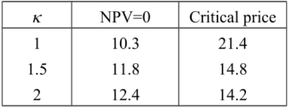
5.2. The investment threshold and the speed of adjustment
If Schwartz’s model leads to more reasonable critical prices than those associated with the one-factor model, it is mainly due to the presence of a speed of adjustment which has an impact on the convenience yield and influences indirectly the spot price, giving the latter a mean reverting tendency. As a result, the price of the underlying asset evolves in a more restricted interval. Table 6 presents the simulations with various speeds of adjustment.
Table 6. Schwartz’s model, critical price as a function of the speed of adjustment
NPV=0 Critical price 1 1.5 2 10.3 11.8 12.4 21.4 14.8 14.2 S = 18 $ ; C = 0.2 ; r = 5% = 0.1 ; S = 0.3 ; C = 0.4 ; = 0.9 ; = 0.1 ; CP = 7$, I0 = 25$
These simulations show that the critical price is a decreasing function of the speed of adjustment associated with the convenience yield. When the magnitude of the speed of adjustment is high, the price returns rapidly to its long run mean. In addition, the results presented in Table 6 underline another advantage of Schwartz’s model. The latter authorizes indeed more varied price curves than the one-factor model. These curves can be for example in backwardation for the nearest expiration date, and then in contango. This is the case, in the example above, when the speed of adjustment is set to 1. In that case, even if the critical price of 21.4 dollars per barrel is higher than the initial spot price of 18 dollars, it is recommended to wait before investing. It is better to wait a decrease in the price, because it will later increase. The suggestion obtained with the optional method is contradictory with the one based on the NPV method, which encourages investing immediately. 5.3. Investment decision and term structure of prices
The study of the investment decisions gives rise to the following remarks.
First of all, the quality of the information provided by Brennan and Schwartz’s model is limited: this model can not be used for all the possible values of the convenience yield. And even if we restrict the variation interval of this variable, the results are sometimes meaningless.
Secondly, one must wonder about the impact of the optional valuation when the term structure of prices is in backwardation. In that case, the opportunity to delay is of little interest, because a decrease of the future spot prices is expected. Yet backwardation can be the most frequent situation in certain markets, like the crude oil market. Therefore, for these markets, the optional method leads to the same alternative that the NPV method: invest now or never. Conversely, for markets characterised by contango, the optional method will lead, either to the immediate investment, either to the wait for a higher price. The project will be abandoned in any case.
S
ECTION6. C
ONCLUSIONThis study shows that the value of a real option and the investment decision strongly depend on the method used for the valuation of the net future cash flows associated with an investment project. Indeed, the simulations indicate that the assumptions on the dynamic behaviour of the state variables in the term structure model have a considerable influence on the project’s value and on the investment decision. The analysis based on the two-factor model can be considered as the most reliable, because the latter provides a convincing representation of the prices term structure for distant maturities, which is not the case of Brennan and Schwartz’s model.
The results give rise to certain prudence towards the use of the optional method for the investment decision. Firstly, the optional method does not seem to be more interesting than the net present value for markets that are most of the time in backwardation. Indeed, in that case, the investor’s choice consists in investing now or never, whatever the criterion retained. Secondly, even with a model a priori pertinent like Schwartz’s model, having no market prices for very distant maturities12, one can not be sure of the liability of the analysis for these expiration dates. Thirdly, the distortions of the term structure of prices can sometimes be frequent and rapid, leading to different investment signals at very close valuation dates.
R
EFERENCESBHAPPU R.R. & GUZMAN J., 1995, « Mineral investment decision making : a study of mining company practices », Engineering and Mining Journal, pp 36-38, July.
BELLALAH M., 1990, « Quatre essais sur l’évaluation des options sur indice et des options sur contrat à terme d’indice », Ph D thesis, University Paris IX.
BELLALAH M., 2001, « Le choix des investissements, les options réelles et l'information : une revue de la littérature » (forthcoming).
BERNANKE B.S., 1983, « Irreversibility, uncertainty, and cyclical investment », The Quarterly Journal of Economics, pp 85-106, February.
BRENNAN M.J. & SCHWARTZ E.S., 1985, « Evaluating natural resources investments », The Journal of Business, vol 58, n°2.
BRENNAN M.J. & TRIGEORGIS L., 1999, Project flexibility, agency, and product market competition : new developments in the theory and application of real options analysis, Oxford University Press. COPELAND T. & ANTIKAROV V., 2001, Real options :a practitioner’s guide, Texere, 320 p.
CORTAZAR G. & SCHWARTZ E.S., 1998, « Monte-carlo evaluation model of an undeveloped oil field », Journal of Energy Finance and Development, vol. 3, n°1, pp 73-84.
CORTAZAR G., SCHWARTZ E.S., & CASASSUS, J., 2001, « Optimal exploration investments under price and geological-technical uncertainty: a real options model »; R & D Management, April, vol. 31, n°2. DIXIT A. & PINDYCK R., 1994, Investment under uncertainty, Princeton University Press.
FRIMPONG S. & J.M. WHITING J.M., 1997, « Derivative mine valuation: strategic investment decisions in competitive markets », Resources Policy, vol 23, n°4, pp 163-171.
GIBSON R. & SCHWARTZ E.S., 1989, « Valuation of long term oil-linked assets », Working Paper, Anderson Graduate School of Management, University of California, Los Angeles.
GRINBLATT M. & TITMAN S., 2001, Financial markets and corporate strategy, 2nd edition, Mc Graw
Hill, 880 p.
LAUTIER D., 2000, « La structure par terme des prix des matières premières : analyse théorique et applications au marché pétrolier » PhD Thesis, Paris IX University.
LAUTIER D. & GALLI A., 2001, « Un modèle de structure par terme des prix du pétrole brut avec comportement asymétrique du rendement d’opportunité » Finéco, vol 11, p 73-95.
LAUTIER A., 2002, « Trois modèles de structure par terme des prix du pétrole brut : une comparaison », Banque et Marchés, mars-avril, n°57.
LAUTIER D., 2003, « Les options réelles, une idée séduisante, un instrument facile à créer mais difficile à valoriser », Economies et Sociétés, mai.
MAJD S. & PINDYCK R.S., 1987, « Time to build, option value, and investment decisions », Journal of Financial Economics, vol 18, pp 7-27.
MCDONALD R. & SIEGEL D., 1986, « The value of waiting to invest », Quarterly Journal of Economics, vol. 101, pp 707-727.
MYERS S.C., 1977, « Determinants of corporate borrowing », Journal of Financial Economics, vol 5, pp 147-175.
PINDYCK R., 1980, « Uncertainty and exhaustible resource markets », Journal of Political Economy, vol. 88, n°6, pp 1203-1225.
PINDYCK R., 1991, « Irreversibility, uncertainty, and investment », Journal of Economic Literature, vol 29, pp 1110-1148, September.
SCHWARTZ E.S., 1997, « The stochastic behavior of commodity prices : implications for valuation and hedging », The Journal of Finance, vol LII, n°3, July.
SCHWARTZ E.S. & SMITH J.E., 2000, « Short-Term Variations and Long-Term Dynamics in Commodity Prices », Management Science, July, vol. 46, n°7, pp 893-912.
TRIGEORGIS T., 1999, Real options, MIT press.
APPENDIX: NUMERICAL RESOLUTION METHOD USED FOR THE VALUATION OF THE REAL OPTIONS ASSOCIATED WITH SCHWARTZ’S MODEL
This appendix presents the method used for the resolution of the valuation equation of the real option associated with Schwartz’s model. This method authorizes the resolution of a partial derivatives equation in two steps, despite the existence of a cross partial derivative. The partial derivatives equation is first of all discretized (1). Then we apply to it an alternate direction method (2).
The value of the option to invest satisfies the following differential equation :
0 ) ( 2 1 2 1 2S2V 2C2V SV S rC V C V V rV C S SC C S CC C SS S with:
/
and : V(S,C,T,T)max
NPV(S,C,T,T),0
The solution of this equation is achieved with a finite difference method: its partial derivatives are replaced by approximations obtained with Taylor expansions. Among the finite difference methods, we retained the Crank-Nicholson method for its stability.
1. DISCRETISATION METHOD
The grid is constituted of the points (ih, jh, nk) in the space (S, C, t), such as: S = ih for
0
i m
C = jh for m/2 j m/2 t = nk for
0
n nn
The option value is represented by a scheme in three dimensions:
j) (i, U = j) (i, V nk) jh, V(ih, t) C, V(S, n n .
1.1. APPROXIMATION OF THE PARTIAL DERIVATIVES
We obtain the approximations applying Taylor expansions around the points i, j, k.
At each period s = T - nk, the first and second order derivatives with respect to S and C, and the derivative with respect to the time are:
Un(i,j)/S
Un(i1, j)Un(i1, j)
/2h
Un(i,j)/C
Un(i,j1)Un(i, j1)
/2h
2Un(i,j)/S2
Un(i1,j)2Un(i, j)Un(i1, j)
/h2
2Un(i, j)/C²
Un(i,j1)2Un(i, j)Un(i,j1)
/h2
2Un(i,j)/SC
Un(i1,j1)Un(i1, j1)Un(i1,j1)Un(i1, j1)
/4h2
Un(i, j)/t
Un(i,j)Un1/2(i, j)
/
k / 2
We define the following operators on the variables:
( 1, ) 2 ( , ) ( 1, )
) , ( 2Un i j Un i j Un i j Un i j S
( , 1) 2 ( , ) ( , 1)
) , ( 2Un i j Un i j Un i j Un i j C
( 1, ) ( 1, )
) , (i j U i j U i j Un n n S
( , 1) ( , 1)
) , (i j U i j U i j Un n n C
( , 1) ( , 1)
= ( 1, 1) ( 1, 1) ( 1, 1) ( 1, 1)
) , (i j U i j U i j U i j U i j U i j U i j U n n n n n n S n C S 1.2. APPROXIMATION OF THE PARTIAL DERIVATIVES EQUATION
Replacing the partial derivatives by their approximation in the partial derivatives equation, we obtain, for each sT
n(1/2)
k, at the points S = ih and C = jh, the following expression:
2
(, ) (, )
) , ( 2 2 4 2 2 2 / 1 2 2 2 2 2 2 j i U j i U k j i U r h jh jh r i h i h i n n n C S C S C S C C S S
1 (, ) (, ) 2 4 4 8 ² 4 4 1 2 / 1 2 2 2 2 2 j i U j i U rk h jh k jh r ik h k i h k k i n n z C S C S C S C C S S zUn1 2/ ( , )i j Un1( , )i j In addition, we have: : Un1/2(i,j)(1/2)
Un1(i,j)Un(i,j)
(z2)Un1(i, j)zUn(i, j)Replacing z with its value, we obtain the system: