Using Choquet integral in Machine learning: What can MCDA bring?

Welcome

Marc Pirlot (UMONS) and Vincent Mousseau (ECP) are welcoming you to the first DA2PL

Work-shop. The aims of this workshop “from multiple criteria decision Aid to Preference Learning” is to

bring together researchers involved in Preference Modeling and Preference Learning and identify

re-search challenges at the crossroad of both rere-search fields.

It is a great pleasure to provide, during two days, a positive context for scientific exchanges and

collaboration : four invited speakers will make a presentation, twelve papers will be presented, and we

will have a poster session and a roundtable. We wish to all participants a fruitful workshop, and an

exiting and enjoyable time in Mons.

Marc Pirlot and Vincent Mousseau

Aim of the workshop

The need for search engines able to select and rank order the pages most relevant to a user’s query

has emphasized the issue of learning the user’s preferences and interests in an adequate way. That is

to say, on the basis of little information on the person who queries the Web, and, in almost no time.

Recommender systems also rely on efficient preference learning.

On the other hand, preference modeling has been an auxiliary discipline related to Multicriteria

de-cision aiding for a long time. Methods for eliciting preference models, including learning by examples,

are a crucial issue in this field.

It is quite natural to think and to observe in practice that preference modeling and learning are

two fields that have things to say to one another. It is the main goal of the present workshop to bring

together researchers involved in those disciplines, in order to identify research issues in which

cross-fertilization is already at work or can be expected. Communications related to successful usage of

explicit preference models in preference learning are especially welcome as well as communications

devoted to innovative preference learning methods in MCDA. The programme of the workshop will

consist of three or four invited lectures and about 15 selected research communications.

Support

This workshop is organized in the framework of the GDRI (Groupement de Recherche

Interna-tional) “Algorithmic Decision Theory”, which is recognized and supported by CNRS (France), FNRS

(Belgium), FNR (Luxemburg).

The support of Fonds de la Recherche Scientifique (FNRS, Belgium), Faculté Polytechnique UMONS,

Ecole Centrale Paris and Belgian Society for Operational Research (SOGESCI-BVWB) is gratefully

acknowledged.

Organization

The DA2PL workshop is jointly organized by Marc Pirlot, University of Mons (UMONS), Faculté

Polytechnique, Belgium, and Vincent Mousseau, Ecole Centrale Paris (ECP), France

The workshop is one in a series of events organized for commemorating the 175th anniversary of

the foundation of the Faculté Polytechnique de Mons

The Faculté was founded in 1837 by A. Devillez and Th. Guibal, two engineers from Ecole

Cen-trale de Paris ! !

It has been the first engineering school in Belgium (under the name “Ecole des Mines du Hainaut”)

Program committee

– Raymond Bisdorff (University of Luxembourg, Luxembourg),

– Craig Boutillier (University of Toronto, Canada),

– Denis Bouyssou (Paris Dauphine University, France),

– Ronen Brafman (Ben Gurion University, Israel),

– Bernard De Baets (Ghent University, Belgium),

– Yves De Smet (Université libre de Bruxelles, Belgium),

– Luis Dias (University of Coimbra, Portugal),

– Philippe Fortemps (University of Mons, Belgium),

– Patrick Meyer (Telecom Bretagne, France),

– Vincent Mousseau (Ecole Centrale, Paris),

– Patrice Perny (Pierre and Marie Curie University, France),

– Marc Pirlot (University of Mons, Belgium),

– Ahti Salo (Aalto University, Finland),

– Alexis Tsoukias (Paris Dauphine University, France),

– Aida Valls (Universitat Rovira I Virgili, Catalonia, Spain),

– Paolo Viappiani (Aalborg University, Denmark)

Organizing committee

– Valérie Brison, MATHRO, Faculté Polytechnique, Université de Mons

– Olivier Cailloux, Laboratoire de Génie Industriel, Ecole Centrale Paris

– Yves De Smet, CODE-SMG, Ecole Polytechnique, Université libre de Bruxelles

– Philippe Fortemps, MATHRO, Faculté Polytechnique, Université de Mons

– Massimo Gurrieri, MATHRO, Faculté Polytechnique, Université de Mons

– Vincent Mousseau, Laboratoire de Génie Industriel, Ecole Centrale Paris, France

– Wassila Ouerdane, Laboratoire de Génie Industriel, Ecole Centrale Paris

– Marc Pirlot, MATHRO, Faculté Polytechnique, Université de Mons

– Xavier Siebert, MATHRO, Faculté Polytechnique, Université de Mons

– Arnaud Vandaele, MATHRO, Faculté Polytechnique, Université de Mons

– Laurence Wouters, MATHRO, Faculté Polytechnique, Université de Mons

P

ROGRAM

Thursday November 15th, 2012

9h00 Registration

9h15 Welcoming Address

9h30 Session 1

– Invited speaker : "Preference Learning : an Introduction", page 1

Eyke Hüllermeier,

Department of Mathematics and Computer Science, Philipps-Universität Marburg, Germany

The topic of "preferences" has recently attracted considerable attention in artificial intelligence

in general and machine learning in particular, where the topic of preference learning has

emer-ged as a new, interdisciplinary research field with close connections to related areas such as

operations research, social choice and decision theory. Roughly speaking, preference learning

is about methods for learning preference models from explicit or implicit preference

informa-tion, typically used for predicting the preferences of an individual or a group of individuals.

Approaches relevant to this area range from learning special types of preference models, such as

lexicographic orders, over “learning to rank” for information retrieval to collaborative filtering

techniques for recommender systems. The primary goal of this tutorial is to survey the field of

preference learning in its current stage of development. The presentation will focus on a

syste-matic overview of different types of preference learning problems, methods and algorithms to

tackle these problems, and metrics for evaluating the performance of preference models induced

from data.

10h30 Coffee break

11h00 Session 2

– “A New Rule-based Label Ranking Method”, pages 3-13

M. Gurrieri

, X. Siebert

, Ph. Fortemps

, S. Greco

and R. Slowinski

MATHRO, Faculté Polytechnique, UMONS,

University of Catania, Italy,

Poznan University of Technology, Poland

This work focuses on a particular application of preference ranking, wherein the problem is to

learn a mapping from instances to rankings over a finite set of labels, i.e. label ranking. Our

ranking (linear order) among labels. The approach presented in this paper mainly comprises

four phases : preprocessing, rules generation, classification and ranking generation.

– “Preference-based clustering of large datasets”, pages 14-20

A. Olteanu

and R. Bisdorff

1

Université du Luxembourg

Clustering has been widely studied in Data Mining literature, where, through different measures

related to similarity among objects, potential structures that exist in the data are uncovered. In

the field of Multiple Criteria Decision Analysis (MCDA), this topic has received less attention,

although the objects in this case, called alternatives, relate to each other through measures of

preference, which give the possibility of structuring them in more diverse ways. In this paper

we present an approach for clustering sets of alternatives using preferential information from a

decision-maker. As clustering is dependent on the relations between the alternatives, clustering

large datasets quickly becomes impractical, an issue we try to address by extending our approach

accordingly.

– “Learning the parameters of a multiple criteria sorting method from large sets of assignment

examples”, pages 21-31

O. Sobrie

, V. Mousseau

and M. Pirlot

LGI, Ecole Centrale Paris,

MATHRO, Faculté Polytechnique, UMONS

ELECTRE TRI is a sorting method used in multiple criteria decision analysis. It assigns each

alternative, described by a performance vector, to a category selected in a set of pre-defined

ordered categories. Consecutive categories are separated by a profile. In a simplified version

proposed and studied by Bouyssou and Marchant and called MR-Sort, a majority rule is used

for assigning the alternatives to categories. Each alternative a is assigned to the lowest category

for which a is at least as good as the lower profile delimiting this category for a majority of

weighted criteria. In this paper, a new algorithm is proposed for learning the parameters of this

model on the basis of assignment examples. In contrast with previous work ([7]), the present

algorithm is designed to deal with large learning sets. Experimental results are presented, which

assess the algorithm performances with respect to issues like model retrieval, computational

efficiency and tolerance for error.

– “A piecewise linear approximation of PROMETHEE II’s net flow scores”, pages 32-39

S. Eppe

and Y. De Smet

1

CoDE, Université Libre de Bruxelles

Promethee II is a prominent outranking method that builds a complete ranking on a set of actions

by means of pairwise action comparisons. However, the number of comparisons increases

qua-dratically with the number of actions, leading to computation times that may become prohibitive

for large decision problems. Practitioners generally seem to alleviate this issue by down-sizing

the problem, a solution that may not always be acceptable though. Therefore, as an alternative,

we propose a piecewise linear model that approximates Promethee II’s net ow scores without

requiring costly pairwise comparisons : our model reduces the computational complexity (with

respect to the number of actions) from quadratic to linear, at the cost of some misranked actions.

Experimental results on artificial problem instances show a decreasing proportion of those

mis-13h00 Lunch

14h30 Session 3

– Invited speaker : “Principled Techniques for Utility-based Preference Elicitation in

Conversa-tional Systems”, page 40

Paolo Viappiani,

CNRS-LIP6, Université Pierre et Marie Curie, Paris

Preference elicitation is an important component of many applications, such as decision support

systems and recommender systems. It is however a challenging task for a number of reasons.

First, elicitation of user preferences is usually expensive (w.r.t. time, cognitive effort, etc.).

Se-cond, many decision problems have large outcome or decision spaces. Third, users are inherently

“noisy” and inconsistent.

Adaptive utility elicitation tackles these challenge by representing the system knowledge about

the user in form of “beliefs” about the possible utility functions, that are updated following user

responses ; elicitation queries can be chosen adaptively given the current belief. In this way, one

can often make good (or even optimal) recommendations with sparse knowledge of the user’s

utility function.

We analyze the connection between the problem of generating optimal recommendation sets and

the problem of generating optimal choice queries, considering both Bayesian and regret-based

elicitation. Our results show that, somewhat surprisingly, under very general circumstances, the

optimal recommendation set coincides with the optimal query.

15h30 Coffee break

16h00 Session 4

– “Using Choquet integral in Machine Learning : what can MCDA bring ?”, pages 41-47

D. Bouyssou

, M. Couceiro

, C. Labreuche

, J.-L. Marichal

and B. Mayag

1

CNRS-Lamsade, Université Paris Dauphine,

Thales,

Université du Luxembourg.

In this paper we discuss the Choquet integral model in the realm of Preference Learning, and

point out advantages of learning simultaneously partial utility functions and capacities rather

than sequentially, i.e., first utility functions and then capacities or vice-versa. Moreover, we

present possible interpretations of the Choquet integral model in Preference Learning based on

Shapley values and interaction indices.

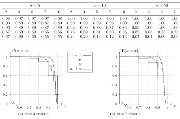
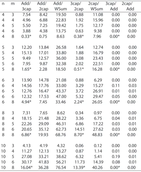
– “On the expressiveness of the additive value function and the Choquet integral models”, pages

48-56

P. Meyer

and M. Pirlot

Institut Télécom, Télécom Bretagne,

MATHRO, Faculté Polytechnique, UMONS

Recent - and less recent - work has been devoted to learning additive value functions or a

Cho-quet capacity to represent the preference of a decision maker on a set of alternatives described

by their performance on the relevant attributes. In this work we compare the ability of related

capacity, an additive value function in general or a piecewise-linear additive value function with

2 or 3 pieces. We also generate non preferentially independent data in order to test to which

extent 2- or 3-additive Choquet integrals allow to represent the given orders. The results explore

how representability depends on varying the numbers of alternatives and criteria.

– “Using set functions for multiple classifiers combination”, pages 57-62

F. Rico

, A. Rolland

,

1

Laboratoire ERIC - Université Lumière Lyon

In machine learning, the multiple classifiers aggregation problems consist in using multiple

clas-sifiers to enhance the quality of a single classifier. Simple clasclas-sifiers as mean or majority rules

are already used, but the aggregation methods used in voting theory or multi-criteria decision

making should increase the quality of the obtained results. Meanwhile, these methods should

lead to better interpretable results for a human decision-maker. We present here the results of a

first experiment based on the use of Choquet integral, decisive sets and rough sets based methods

on four different datasets.

– “Preference Learning using the Choquet Integral”, page 63

E. Hüllermeier

1

Department of Mathematics and Computer Science, Philipps-Universität Marburg, Germany

This talk advocates the (discrete) Choquet integral as a mathematical tool for preference

lear-ning. Being widely used as a flexible aggregation operator in fields like multiple criteria decision

making, the Choquet integral suggests itself as a natural target for learning preference models.

From a machine learning perspective, it can be seen as a generalized linear model that combines

monotonicity and flexibility in a mathematically sound and elegant manner. Besides, it exhibits

a number of additional features, including suitable means for supporting model interpretation.

The learning problem itself essentially comes down to specifying the fuzzy measure in the

inte-gral representation on the basis of the preference data given. The talk will specifically address

theoretical as well as methodological and algorithmic issues related to this problem. Moreover,

applications to concrete preference learning problems such as instance and object ranking will

be presented.

Friday November 16th, 2012

9h Session 5

– Invited speaker : “Ranking Problems, Task Losses and their Surrogates”, page 65

Krzysztof Dembczynski,

Laboratory of Intelligent Decision Support Systems, Poznan University of Technology

From the learning perspective, the goal of the ranking problem is to train a model that is able

to order a set of objects according to the preferences of a subject. Depending on the

prefe-rence structure and training information, one can distinguish several types of ranking problems,

like bipartite ranking, label ranking, or a general problem of conditional rankings, to mention

a few. To measure the performance in the ranking problems one uses many different evaluation

metrics, with the most popular being Pairwise Disagreement (also referred to as rank loss),

Dis-counted Cumulative Gain, Average Precision, and Expected Reciprocal Rank. These measures

a near-optimal solution with respect to a given task loss. For simple ranking problems and some

task losses the answer is positive, but it seems that in general the answer is rather negative.

Du-ring the talk we will discuss several results obtained so far, with the emphasis on the bipartite

and multilabel ranking problem and the pairwise disagreement loss, in which case very simple

surrogate losses lead to the optimal solution.

10h00 Coffee break + Poster session

– "Preference Learning to Rank : An Experimental Case Study", M. Abbas, USTHB, Alger,

Al-gerie

– "From preferences elicitation to values, opinions and verisimilitudes elicitation", I. Crevits, M.

Labour, Université de Valenciennes- pages 66-73

– "Group Decision Making for selection of an Information System in a Business Context", T.

Pereira, D.B.M.M Fontes, Porto, Portugal - pages 74-82

– "Ontology-based management of uncertain preferences in user profiles", J. Borras, A. Valls, A.

Moreno, D. Isern, Universitat Rovira i Virgili, Tarragona - pages 83-89

– "Optimizing on the efficient set. New results", D. Chaabane, USTHB, Alger, Algerie

11h00 Session 6

– Roundtable : "From Multiple Criteria Decision Analysis to Preference Learning"

Participants : E. Hüllermeier, P. Viapianni, K. Dembczynski

12h00 Lunch

13h30 Session 7

– Invited speaker : “Learning GAI networks”, page 90

Yann Chevaleyre,

LIPN, Université Paris 13

Generalized Additive Independence (GAI) models have been widely used to represent utility

functions. In this talk, we will address the problem of learning GAI networks from pairwise

preferences. First, we will consider the case where the structure of the GAI network is known of

bounded from above. We will see how this problem can be reduced to a kernel learning problem.

Then, we will investigate the structure learning problem. After presenting the computational of

algorithms can be used to solve this problem.

14h30 Coffee break

15h00 Session 8

– “On measuring and testing the ordinal correlation between valued outranking relations”, pages

91-100

R. Bisdorff

,

University of Luxembourg

– “Elicitation of decision parameters for thermal comfort on the trains”, pages 101-107

L. Mammeri

, D. Bouyssou

, C. Galais

, M. Ozturk

, S. Segretain

and C. Talotte

CNRS-Lamsade, Université Paris-Dauphine,

SNCF

We present in this paper a real world application for the elicitation of decision parameters used in

the evaluation of thermal comfort in high speed trains. The model representing the thermal

com-fort is a hierarchical one and we propose to use different aggregation methods for different levels

of the model. The methods used are rule-based aggregation, Electre Tri and 2-additive Choquet.

We show in this paper the reasons of the choice of such methods and detail the approach used

for the elicitation of the parameters of these methods.

– “Dynamic managing and learning of user preferences in a content-based recommender system”,

pages 108-114

L. Marín

, A. Moreno

, D. Isern

and A. Valls

Universitat Rovira i Virgili, Tarragona

The main objective of the work described in this paper is to design techniques of profile learning

to enable a Recommender System to automatic and dynamically adapt preferences stored about

the users in order to increase the accuracy of the recommendations. The alternatives (or set of

possible solutions to the recommendation problem) are defined by multiple criteria that can be

either numerical or categorical. A study of the performance of the whole designed techniques so

far is also included.

– “An algorithm for active learning of lexicographic preferences”, pages 115-122

F. Delecroix

, M. Morge

, J.-Chr. Routier

1

Université Lille 1

At the crossroad of preference learning and multicriteria decision aiding, recent research on

preference elicitation provide useful methods for recommendation systems. In this paper, we

consider (partial) lexicographic preferences. In this way, we can consider dilemmas and we

show that these situations have a minor impact in practical cases. Based on this observation, we

propose an algorithm for active learning of preferences. This algorithm solve the dilemmas by

suggesting concrete alternatives which must be ranked by the user.

Session 1

Invited speaker : Eyke Hüllermeier

Department of Mathematics and Computer Science, Philipps-Universität Marburg, Germany

"Preference Learning : an Introduction",

The topic of "preferences" has recently attracted considerable attention in artificial intelligence

in general and machine learning in particular, where the topic of preference learning has

emer-ged as a new, interdisciplinary research field with close connections to related areas such as

operations research, social choice and decision theory. Roughly speaking, preference learning

is about methods for learning preference models from explicit or implicit preference

informa-tion, typically used for predicting the preferences of an individual or a group of individuals.

Approaches relevant to this area range from learning special types of preference models, such as

lexicographic orders, over “learning to rank” for information retrieval to collaborative filtering

techniques for recommender systems. The primary goal of this tutorial is to survey the field of

preference learning in its current stage of development. The presentation will focus on a

syste-matic overview of different types of preference learning problems, methods and algorithms to

tackle these problems, and metrics for evaluating the performance of preference models induced

from data.

Session 2

– “A New Rule-based Label Ranking Method”,

M. Gurrieri

, X. Siebert

, Ph. Fortemps

, S. Greco

and R. Slowinski

MATHRO, Faculté Polytechnique, UMONS,

University of Catania, Italy,

Poznan University of Technology, Poland

– “Preference-based clustering of large datasets”,

A. Olteanu

and R. Bisdorff

Université du Luxembourg

– “Learning the parameters of a multiple criteria sorting method from large sets of assignment

examples”,

O. Sobrie

, V. Mousseau

and M. Pirlot

LGI, Ecole Centrale Paris,

MATHRO, Faculté Polytechnique, UMONS

– “A piecewise linear approximation of PROMETHEE II’s net flow scores”,

S. Eppe

and Y. De Smet

1

Reduction from Label Ranking to Binary Classification

Massimo Gurrieria,1_{, Xavier Siebert}a_{, Philippe Fortemps}a_{, Salvatore Greco}b_{; Roman Słowiński}c

a

UMons, Rue du Houdain 9, 7000 Mons, Belgium

b_{Faculty of Economics, University of Catania, Corso Italia 55, 95129 Catania, Italy} c

Institute of Computing Science, Poznan University of Technology, 3A Piotrowo Street, 60-965 Poznan, Poland

Abstract. This work focuses on a particular application of preference learning, wherein the problem is to learn a mapping from instances to rankings over a finite set of labels, i.e. label ranking. Our approach is based on a learning reduction technique to reduce label ranking to binary classification. The proposed reduction framework can be used with different binary classification algorithms in order to solve the label ranking problem. In particular, in this paper, we present two variants of this reduction framework, one where Multi-Layer Perceptron is used as binary classifier and another one where the Dominance-based Rough Set Approach is used. In the latter, on the one hand it is possible to deal with possible monotonicity constraints and on the other hand it is possible to provide such a mapping (i.e. a label ranker) in the form of logical rules: if [antecedent] then [consequent], where [antecedent] contains a set of conditions, usually connected by a logical conjunction operator (AND), while [consequent] consists in a ranking (linear order) among labels.

Keywords: Label Ranking, Preference Learning, Decision Rules, Dominance-based Rough Set Approach.

1

Introduction

Preference learning [6] is a relatively new topic that is gaining increasing attention in data mining and re-lated fields [8, 9, 10]. The most challenging aspect of this topic is the possibility of predicting weak or partial orderings of labels, rather than single val-ues which is typical of classification problems. Pref-erence learning problems are typically distinguished in three topics: object ranking, instance ranking and label ranking. Object ranking consists in finding a ranking function F whose input is a set X of in-stances characterized by attributes and whose out-put is a ranking of this set of instances, in the form of a weak order [6]. Such a ranking is typically ob-tained by giving a score to each x ∈ X and by or-dering instances with respect to these scores. The training process takes as input either partial rank-ings or pairwise preferences between instances of X. Such a kind of problem is also commonly studied in

the field of Multi-Criteria Decision Aid (e.g. the so-called Thierry’s choice problem) [19]. In the context of instance ranking [6], the goal is to find a ranking function F whose input is a set X of instances char-acterized by attributes and whose output is a rank-ing of this set (again a weak order on X). However, in contrast with object ranking, each instance x is associated with a class among a set of classes C= {C1; C2; ...; Ck} and this set is furthermore ordered

(nominal, quantitative or qualitative scales), there-fore: {C1  C2  ...  Ck}. The output of such

a kind of problem consists in rankings wherein in-stances labeled with higher classes are preferred to (or precede) instances labeled with lower classes. This problem is similar to the problem of sorting in the field of Multi-Criteria Decision Aid (e.g. the contact lenses problem) [19]. The learning scenario discussed in this paper concerns a set of training instances (or examples) which are associated with rankings over a finite set of labels, i.e. label ranking [4, 5, 6, 7].

This paper is organized as follows. In Section 2, we introduce the label ranking topic and existing ap-proaches as well. In particular, we discuss existing learning reduction techniques. In Section 3, we illus-trate our reduction framework to reduce label ranking to binary classification and the general classification and ranking generation phases according to our pro-posed label ranking method. In Section 4, we illus-trate two applications of our reduction framework: an application based on the Variable Consistency Dominance-based Rough Set Approach (VC-DRSA) that provides predictions on rankings in the form of decision rules; and an application based on the Multi-Layer Perceptron Algorithm (MLP). In Section 5, we present experimental results that we conducted with three different configurations of our framework. Fi-nally, we present some conclusions in Section 6.

2

Label Ranking

In label ranking, the main goal is to predict for any instance x, from an instance space X, a preference relation x: X → L where L= {λ1; λ2; ...; λk} is a set

of labels or alternatives, such that λi x λj means

that instance x prefers label λi to label λj. More

specifically, we are interested in the case where x

is a total strict order over L, that is, a ranking of the entire set L. Such ranking x can be therefore

identified with a permutation πxof {1, 2, ..., k} in the

permutation space Ω of the index set of L, such that πx(i) < πx(j) means that label λi is preferred to

la-bel λj (πx(i) represents the position of label λiin the

ranking). A complete ranking (i.e. a linear order) for the set L is therefore given by:

λ_π−1

x (1)xλπ−1x (2)x... xλπx−1(k) (2.1)

where π−1x (j), j = 1, 2, ...k, represents the index of

the label that occupies the position j in the ranking. In order to evaluate the accuracy of a model (or label ranker), once the predicted ranking π0 for an instance x has been established, it has to be compared to the actual true ranking π associated to the instance x, by means of an accuracy measure defined on Ω, the permutation space over L. As explained in [4], it is possible to associate an instance x to a probability distribution P(.|x) over the set Ω so that P(τ |x) is

(as in the setting of classification) is typically mea-sured by means of its expected loss on rankings:

E(D(τx, τx0)) = E(D(τ, τ0)|x) (2.2)

where D(., .) is a distance function (between permu-tations in our setting) and τx and τx0 are the true

outcome and the prediction made by the model M respectively. Given such a distance metric (i.e. loss function) to be minimized, the best prediction is:

τ∗= arg min

τ0_∈Ω

X

τ ∈Ω

P(τ |x)D(τ0, τ ). (2.3)

Spearman’s footrule and Kendall’s tau are two well known distances between rankings. In a celebrated result [24], it is showed that Spearman’s footrule and Kendall’s tau are always within a factor of two from each other. Given two permutations τ, τ0 ∈ Ω, the Spearman’s footrule distance is given by:

F (τ, τ0) =

k

X

i=1

|τi− τi0| (2.4)

and measures the total element-wise displacements between two permutations. The Kendall’s tau dis-tance is instead given by:

K(τ, τ0) = #{(i, j) : i < j|τi> τj∧ τi0< τ 0

j} (2.5)

and measures the total number of pairwise inversions between two permutations. By performing a linear scaling of K(τ, τ0) to the interval [−1, +1], it is pos-sible to define the Kendall’s tau coefficient:

τk =

nc− nd

k(k − 1) 2

(2.6)

where nc and nd are the numbers of concordant and

discordant pairs of labels, respectively. The sum of squared rank distances is also typically used as a dis-tance metric: S(τ, τ0) = k X i=1 (τi− τi0) 2 (2.7)

and by performing a normalization in the interval [−1, +1], it is possible to define the Spearman rank correlation which is a similarity measure between two permutations (rankings):

k

P_(τ

2.1 Label Ranking Approaches

There are two main groups of approaches to label ranking. On the one hand, we have decomposition (or learning reduction) methods, such as Constraint Classification [3] and Ranking by Pairwise Compar-isons [4], that transform the original label ranking problem into a new binary classification problem. On the other hand, we have direct methods that mainly adapt existing classification algorithms, such as De-cision Trees and Instance-based learning [5] (both being lazy methods), Boosting algorithms [11] and Support Vector Machines (SVM) [12], to treat the rankings as target objects without any transforma-tion over the data set. There also exists an adap-tation [21] of the association rule mining algorithm APRIORI for label ranking based on similarity mea-sures between rankings and where the label ranking prediction is given in the form of Label Ranking As-sociation Rules: A → π, where A ⊆ X and π ∈ Ω. The main idea of this method is that the support of a ranking π increases with the observation of similar rankings πi. In this manner it is possible to assign

a weight to each ranking πi in the training set that

represents its contribution to the probability that π may be observed.

2.2 Learning Reduction Techniques

As already mentioned, decomposition methods trans-form the original label ranking problem into one or several binary classification problems, a process that is called learning reduction which is a generalization of approaches to multi-label classification [6, 12]. In the approach Constraint Classification [3], a utility linear function fi(x) = wi• x is associated to each

la-bel λi, ∀i ∈ {1, 2, ..., k} and to an instance x ∈ X and

where wi = (wi

1, ..., wli) is an l-dimensional vector

consisting of label coefficients associated with label λi. The goal is then to find a linear sorting function:

h(x) = argsorti=1,2,...,kfi(x) (2.9)

which returns a permutation of the index set {1, 2, ..., k} of labels. A preference of the form λix

λj is accordingly converted into a positive constraint

fi(x) − fj(x) > 0 or, equivalently, into a negative one

fj(x) − fi(x) < 0. In this approach, label ranking

can be reduced to binary classification by means of Kesler’s construction [8]. Constraints can be related to the sign of the inner product: < z, W >, wherein:

1 k 1 1 k k

is an (k × l)-dimensional vector representing the con-catenation of all label coefficients and z is a (k × l)-dimensional vector whose components are defined as follows. If for an instance x, λi x λj holds,

the components of vector z with index ranging from ((i − 1) × l) + 1 to (i × l) are filled with the compo-nents of instance x; compocompo-nents with index ranging from ((j −1)×l)+1 to (j ×l) are filled with the oppo-site of components of instance x; and the remaining entries are filled with 0’s. A further component with 1 is added in order to have a positive classification instance. A negative instance is obtained by consid-ering reversed signs. In such a way, each instance x will generate an expanded set P(x) given by the union of positive and negative instances. Finally, the entire set of preference instances X generates an expanded training set:

P(X) = ∪x∈X(P (x)) (2.11)

that is linearly separable by learning a separating hy-perplane with any binary classifier. A very impor-tant aspect of this approach is that it takes into ac-count the correlation between labels, since the learn-ing dataset contains the overall information about labels. However, this model is very complex and the preprocessing part is quite cumbersome. Kesler’s con-struction multiplies the dimensionality of the data by k and the number of samples by k − 1, where k is the cardinality of the label set. It is clear that direct use for training a classifier is in practice not attrac-tive. In Ranking by Pairwise Comparison (RPC) [4], instead, the main idea is to explode the original label ranking problem to several independent binary clas-sification problems and to learn a binary classifier for each pair of labels. More particularly, each preference information of the form λi x λj is considered as a

training instance for a learner Mi,j which outputs 1

if λi xλj holds, 0 otherwise. If L= {λ1; λ2; ...; λk},

the number of learners is at most k(k − 1)/2. The label ranking associated to a new instance is then obtained by means of a voting strategy, wherein each label is, for example, evaluated by summing scores of all learners and then ordered with respect to this evaluation. However the main drawback of this ap-proach is that it trains independent binary classifiers which cannot take into account relations (i.e.

corre-3

Reduction Framework

3.1 Preprocessing: from Label Ranking to Binary Classification

In this section, a general reduction framework is pro-posed to reduce label ranking to binary classification. Consequently, the proposed reduction framework can be used with different binary classifiers (two variants will be presented in Section 4). In the preprocessing phase, the original label ranking dataset is converted into a new dataset where the original ranking πx is

split into pairwise preference relations. Though the proposed reduction technique is very similar to the one presented in [4], in the latter each pair of labels is treated separately so that k(k − 1)/2 independent binary classifiers are trained during the training pro-cess. By contrast, in our reduction framework, a sgle classifier is trained and the overall preference in-formation is treated at once in a single dataset, simi-larly to the reduction schemes used in [25] or in [26]. The original dataset is a set of instances T = {(x, πx)}, where x and πx represent, respectively,

the feature vector and the corresponding target la-bel ranking associated with the instance x. The feature vector x is in fact an l-dimensional vec-tor (q1, q2, ..., ql) of attributes (typically

numeri-cal values), so that: (x, πx) = (q1, q2, ..., ql, πx).

Each original instance (x, πx) = (q1, q2, ..., ql, πx) is

transformed into a set of new (simpler) instances {x1,2, x1,3, ..., xi,j, ...} where:

xi,j= (q1, q2, ..., ql, p, d) (3.1)

with i, j ∈ {1, 2, ..., k}, i < j, p ∈ {(λ1, λ2), ..., (λk−1, λk)} and d ∈ {−1, +1}.

This is obtained by splitting the original set of labels into k(k − 1)/2 pairs of labels and by consid-ering an additional nominal attribute p, called re-lation attribute, whose possible values are all pairs of labels. A decisional attribute d ∈ {−1; +1} is added to take into account the preference relation between two given labels (λi,λj), represented by the

value of relation attribute p, according to the rank-ing πx. This decision attribute d says in which

man-ner the pair (λi, λj) has to be considered during the

training process. In other words, if for the instance (x, πx), we want to treat the pair (λi, λj), then we

set p = (λi, λj). Moreover, if λi is preferred to λj

then d = +1, otherwise if λj is preferred to λi then

d = −1. For example, the instance:

generates the following set of simpler instances (i.e., a new instance for each possible pair of labels):

x1,2= (−1.5, 2.4, 1.6, (λ1, λ2), −1) x1,3= (−1.5, 2.4, 1.6, (λ1, λ3), +1) x2,3= (−1.5, 2.4, 1.6, (λ2, λ3), +1).

The total number of training instances obtained at the end of the reduction (3.1) is nk(k−1)₂ , where n is the number of original training instances and k is the number of labels, while the total number of attributes is l+1 where l is the number of original attributes. By using this reduction framework (3.1), it is therefore possible to treat pair-wise preference information at once in a single dataset where correlations between labels are taken into account simultaneously.

3.2 Classification Process

The classification of an unknown instance x0 (i.e. ei-ther a testing instance or a new instance to be sified) can be performed by using some binary clas-sifier capable of estimating conditional probabilities (e.g. multilayer perceptron algorithm):

P(λix0 λ_j) = P(d = 1|x0a_i,j), (3.2)

P(λj x0 λ_i) = P(d = −1|x0a_i,j), (3.3)

where x0a_i,jis the feature vector of x0that is augmented with the relation attribute p = (λi, λj), therefore:

x0ai,j = (q1, q2, ..., ql, p). (3.4)

By using these conditional probabilities, it is possible to define scores:

Γ_(i,j)+ _{= P(λ}ix0 λ_j) (3.5)

Γ_(i,j)− _{= P(λ}jx0 λ_i). (3.6)

Scores (3.5) and (3.6) represent the probability that for the instance x0 label λiis ranked higher (preferred

to) than λjand the probability that label λjis ranked

higher (preferred to) than λi, respectively.

3.3 Ranking Generation Process

The final step of our approach concerns the genera-tion of a final ranking (i.e. a linear order) among the entire set of labels for the new instance x0, based on the preference relation x0 learned during the

classi-fication process. On the one hand, for each pair of la-bels (λi, λj), i, j ∈ {1, 2, ..., k}, i < j, a decision d(x0)

asymmetric, irreflexive but, in general, not transitive (i.e. cycles are likely to happen). In order to over-come cycles, a Net Flow Score procedure [22] is used to aggregate pairwise preferences. This procedure al-lows to obtain a linear order among the entire set of labels since each label λi is evaluated by considering

the following score:

S(i) =X

j6=i

(Γ_(i,j)+ − Γ_(i,j)− ), (3.7)

where Γ_(i,j)+ and Γ_(i,j)− are given by (3.5) and (3.6). The final ranking τ is therefore obtained by ordering labels according to decreasing values of scores (3.7) (the higher the score, the higher the preference in the ranking): S(i) > S(i) ⇔ τi< τj.

4

Applications of Reduction

Framework

In this section, we discuss two variants of our reduc-tion framework: an applicareduc-tion based on the Variable Consistency Dominance-based Rough Set Approach (VC-DRSA) that provides predictions on rankings in the form of rules; and a variant based on the Multi-Layer Perceptron Algorithm (MLP).

4.1 VC-DRSA for Label Ranking

This variant is based on the rule induction paradigm, i.e. a variant that can provide predictions on rank-ings in the form of decision rules: Φ → Ψ . The rule learner used in this variant is VC-DRSA [13, 14, 15] which is an extension of the Dominance-based Rough Set Approach (DRSA) [2, 23]. The motivation behind this variant is twofold: on the one hand it is due to the fact that most of available methods, though are very efficient algorithms, they lack transparency and mostly perform like "black boxes", i.e. just like ora-cles which never clearly show relationships between input and output. From this point of view, it seems natural to provide a label ranker in the form of logi-cal rules. It is well known, in fact, that rules clearly show relationships between the feature vector (the antecedent Φ) and the associated output (the con-sequent Ψ ), since both are visible in the rule syntax. As a consequence, rules are very easy to interpret and can provide very rich and complete information, es-pecially in the field of decision aid [16, 19, 20].

How-hand, the choice of VC-DRSA as a rule learner is also motivated by the potential requirement that an explicit order in the input space (i.e. value-order of attributes) could be used to monotonically establish an order among labels in the output space (i.e. label ranking with monotonicity constraints). We describe in the following the reduction process proposed in this variant which is sligtly different from the reduc-tion (3.1).

Each original instance (x, πx) = (q1, q2, ..., ql, πx)

is transformed into a set of new (simpler) instances {x1,2, x1,3, ..., xi,j, ...} where: xi,j= (q1≥, q ≤ 1, q ≥ 2, q ≤ 2, ..., q ≥ l , q ≤ l , p, d) (4.1) with i, j ∈ {1, 2, ..., k}, i < j, p ∈ {(λ1, λ2), ..., (λk−1, λk)} and d ∈ {GT, LT }.

The main difference consists in transforming each attribute qh into a gain and a cost criterion

q_h≥, q_h≤, h ∈ {1, 2, ..., l}, to be maximized and mini-mized, respectively. This can be justified by the fact that the monotonic relationship between a certain at-tribute and the preference relation between labels is generally unknown. However, in case such a relation is known, one can set a given attribute to be only a gain (cost) criterion. A decisional gain criterion d ∈ {GT ; LT } (i.e., respectively, greater than and less than, where GT  LT ) is finally added to take into account the preference relation between two labels (λi,λj), according to the ranking πx. This decision

criterion says in which manner the relation attribute p = (λi, λj) has to be considered for a given instance

x. In other words, if for the instance (x, πx), λi is

preferred to λj, then d = GT , otherwise d = LT . For

example, the instance:

x = (−1.5, 2.4, 1.6, λ2 λ1 λ3)

generates the following set of simpler instances (i.e., a new instance for each possible pair of labels):

x1,2= (−1.5≥, −1.5≤, 2.4≥, 2.4≤, 1.6≥, 1.6≤, (λ1, λ2), LT ) x1,3= (−1.5≥, −1.5≤, 2.4≥, 2.4≤, 1.6≥, 1.6≤, (λ1, λ3), GT ) x2,3= (−1.5≥, −1.5≤, 2.4≥, 2.4≤, 1.6≥, 1.6≤, (λ2, λ3), GT )

Thus, the original label ranking problem is trans-formed into a simpler binary classification problem wherein each training instance is represented by cri-teria instead of attributes, an additional nominal at-tribute (relation atat-tribute) p and a decisional criterion d ∈ (GT, LT ). The final dataset, as shown in Table 1, contains n × [k(k − 1)/2] training instances while the number of conditional criteria is 2l + 1, where l is the number of original conditional attributes, n is the

q≥₁ q≤₁ .. .. .. q≥_l q≤_l Relation Decision x1,2 q1 q1 .. .. .. ql ql (λ1, λ2) d x1,3 q1 q1 .. .. .. ql ql (λ1, λ3) d ... .. .. .. .. .. .. .. .. ... xk−1,k q1 q1 .. .. .. ql ql (λk−1, λk) d ... .. .. .. ... ... .. .. .. ...

Table 1. Learning Reduction Scheme

4.1.1 Classification Rules As already men-tioned, classification rules are sentences of the form:

Φ → Ψ

where Φ is called the "antecedent" and Ψ is called the "consequent". Φ is typically composed of condi-tions on the values of some attributes, while Ψ is gen-erally the class to which an instance satisfying the antecedent should be assigned. More complex "an-tecedent" and "consequent" forms exist as well. For example, in DRSA the antecedent is a conjunction of elementary conditions concerning one or more crite-ria (either gain or cost critecrite-ria) while the consequent relates to either the upper union of totally ordered classes Cl_t≥ or the downard union of totally ordered classes Cl_t≤. When generating rules, two important measures (among others) are usually taken into ac-count to evaluate the quality of a rule. Such mea-sures are confidence and strength. Let H be the set of training instances verifying the antecedent of a rule r: Φ → Ψ and K the set of training instances ver-ifying the consequent of the rule. We say that rule r holds in the set X with confidence c = |H∩K|_|H| if c is the percentage of instances in H that verify the consequent Ψ . On the other hand, rule r has strength s = |H∩K|_|X| if s is the percentage of instances in X that verify both the antecedent and consequent. Finally, the number |H ∩ K| represents the support of rule r. In the field of Rough Set Rule Induction several algo-rithms have been developed in order to generate rules based on the Rough Set Approach (RSA) [1], such as: AQ, LEM2, MLEM2, DomLEM, VC-DomLEM [13, 16, 17]. Such algorithms are typically based on the scheme of a sequential covering [18] and heuristically generate a minimal set of rules covering instances.

4.1.2 The Training Process: Inferring Rules The second phase of our method consists in the

infer-is obtained by using VC-DomLEM whose complex-itity is polynomial [2]. Let l be the number of at-tributes and n the number of instances in the original data set, the complexity of the algorithm is given by nl(n + 1)(l + 1)/4 and therefore, the time complexity of the algorithm is in O(n2_l2_{). This algorithm}

heuris-tically searches for rules that satisfy a given threshold value of consistency. The applied heuristic strategy is called sequential covering or separate and conquer. It constructs a rule that covers a subset of train-ing instances, removes the covered instances from the training set and iteratively learns another rule that covers some of the remaining instances, until no un-covered instances remain. VC-DomLEM induces an approximately minimal set of minimal decision rules covering all training instances. Since each training in-stance is considered with each possible pair of labels, the training process ends up with a set of minimal and non-redundant decision rules R covering each possi-ble pair of labels. This set R is comprised of subsets R(1,2), R(1,3), ..., R(k−1,k)(one for each pair of labels),

where the generic subset R(i,j), i, j ∈ {1, 2, ..., k}, i <

j, contains the set of rules R(i,j,GT ) for which the

decision d associated with the pair (λi, λj) is GT

and the set of rules R(i,j,LT ) for which d = LT .

It is obviuos that R(i,j) = R(i,j,GT )∪ R(i,j,LT ) and

R(i,j,GT )∩ R(i,j,LT )= ∅.

4.1.3 Computational Complexity We discuss here the computational complexity of the rule in-ference process associated to the proposed method. Firstly, we find the number of training instances that are obtained by using the learning reduction tech-nique (4.1) since the total computational complexity depends on this number as well as on the complexity of the rule learner used for processing these instances and generating rules.

Theorem 1 The time complexity of the inferring rule algorithm (after the learning reduction (4.1))

number of original training instances, k is the num-ber of labels and l is the original numnum-ber of attributes.

Proof. By applying the reduction (4.1), each origi-nal training instance is split into a set of simpler in-stances {x1,2, x1,3, ..., xi,j, ...} which contains exactly

k(k−1)

2 new instances (one for each possible pair). As

a consequence, the total number of training instances obtained at the end of the reduction (3.1) is nk(k−1)₂ , where n is the number of original training instances and k is the number of labels. Moreover, the total number of attributes is 2l + 1 where l is the number of original attributes. Since the time complexity of VC-DomLEM is given by O(nl(n+1)(l+1)₄ ) [2], by re-placing n and l with nk(k−1)₂ and 2l + 1, respectively, the total computational complexity of the inferring rules process is O((n k(k−1) 2 )(2s+1)(n k(k−1) 2 +1)(2l+2) 4 ). u t

4.1.4 The Classification Process The classifi-cation process for an unknown instance x0 (i.e. either a testing instance or a new instance to be classified) is performed by means of the set R and aims at pro-viding a decision (either GT or LT ) for each pair of labels (λi, λj), i, j ∈ {1, 2, ..., k}, i < j. The

clas-sification is performed by considering the following scheme for every pair (i, j) ∈ {1, 2, ..., k}, i < j. Let be R(i,j)the set of rules concerning the pair (λi, λj) and

R(i,j,GT ), R(i,j,LT ) ⊆ R(i,j) subsets having d = GT

and d = LT as decision for the given pair of labels, respectively. For any rule r ∈ R(i,j), we define the

weight: ωr= Sr Si,j (4.2) where Si,j = P r∈Ri,j

Sr and Sr is the support of rule

r. By using weight (4.2), we define these two scores:

W_(i,j)+ = X r∈R(i,j,GT ) ωr (4.3) W_(i,j)− = X r∈R(i,j,LT ) ωr. (4.4)

These two scores represent the total sum of weights of rules for which d = GT and d = LT hold, respec-tively, for the pair (λi, λj). Let define, for the testing

instance x0:

By testing the antecedent of rule r with x0a_i,j, it is possible to define: Ti,j= X r∈Ri,j ωr· δx 0 r (4.6) with δx0 r =    1 if x0a_i,j supports r, 0 otherwise

. The value Ti,j is

the sum of weights of rules supported by x0 for the corresponding pair of labels. Finally, we define:

α+_(i,j)= X r∈R(i,j,GT ) ωr· δx 0 r (4.7) α−_(i,j)= X r∈R(i,j,LT ) ωr· δx 0 r (4.8)

which are, respectively, the total sum of weights of rules, supported by x0, for which d = GT and d = LT hold for the pair (λi, λj). Finally, by normalizing

weights (4.7),(4.8) in [0,1], we define these two scores:

Γ_(i,j)+ = α+_(i,j) Ti,j (4.9) Γ_(i,j)− = α−_(i,j) Ti,j (4.10)

For a given unknown instance x0 (testing instance) and ∀(λi, λj), the classification process provides

scores Γ_(i,j)+ , Γ_(i,j)− . Scores (4.9), (4.10) verify these properties:

Γ_(i,j)+ = Γ_(j,i)− (4.11)

Γ_(i,j)+ , Γ_(i,j)− ∈ [0, 1] (4.12)

Γ_(i,j)+ + Γ_(i,j)− = 1 (4.13)

So that scores (4.9) and (4.10) can be considered as the probability that for the instance x0 label λi is

ranked higher (preferred to) than λj and the

prob-ability that label λj is ranked higher (preferred to)

than λi, respectively. That is:

4.1.5 Classification Scheme I: Majority Class The classification process for a new instance x0 con-sists in finding a decision GT or LT for each possible pair of labels (λi, λj), i, j ∈ {1, 2, ..., k}, i < j, by

test-ing the subset of rules Ri,j. If x0 matches at least one

rule from Ri,j, the final decision for the pair (λi, λj) is

chosen by comparing scores (4.9) and (4.10). The de-cision d(x) is chosen according to max(Γ_(i,j)+ , Γ_(i,j)− ). In case, for a certain pair of labels (λi, λj), x0 does

not match any rule from Ri,j, the model R is silent

w.r.t. this pair and therefore the prediction cannot be provided. Two different strategies are presented in this paper in order to deal with this problem.

In the first strategy, we consider a voting proce-dure consisting in finding the majority class, either GT or LT , for the pair (λi, λj). The majority class

is determined by using scores (4.3) and (4.4) and a default decision for x0 is associated with the higher score. The classification of instance x0for each pair of labels (λi, λj), i, j ∈ {1, 2, ..., k}, i < j, can be

sum-marized by the following scheme: If Γ_(i,j)+ = Γ_(i,j)− = 0 : d(x0) =    GT if W_(i,j)+ ≥ W_(i,j)− ; LT otherwise Else: d(x0) =    GT if Γ_(i,j)+ ≥ Γ_(i,j)− ; LT otherwise

4.1.6 Classification Scheme II: One Nearest Neighbor The second strategy is based on the One Nearest Neighbor scheme (1NN). If for a new in-stance x0 the prediction (decision) d(x0) for a certain pair of labels cannot be provided by the model R, the nearest testing instance x∗ is selected from the training set (the Euclidean distance is used as the distance metric) and d(x0) = d(x∗). Moreover, x0 is associated with same the scores as x∗. The classifi-cation of instance x0 for each pair of labels (λi, λj),

i, j ∈ {1, 2, ..., k}, i < j, can be summarized by the following scheme:

If Γ_(i,j)+ = Γ_(i,j)− = 0 :

d(x0) = d(x∗),

(where x∗ is the nearest neighbor of x0 in the training set) Else: d(x0) =    GT if Γ_(i,j)+ ≥ Γ_(i,j)− ; LT otherwise

4.1.7 Ranking Generation Process The rank-ing generation process is the same as the one dis-cussed in 3.3. As disdis-cussed above, the set of rules R provides, for each pair of labels (λi, λj), i, j ∈

{1, 2, ..., k}, i < j, a decision d(x0_{) and scores (4.9)}

and (4.10), which can be approximated with condi-tional probabilities (4.14), (4.15). The final ranking τ is therefore obtained by ordering labels accord-ing to decreasaccord-ing values of scores (3.7) (the higher the score, the higher the preference in the ranking): S(i) > S(i) ⇔ τi< τj.

4.2 Multi-layer Perceptron for Label Ranking

As discussed above, our reduction framework can be used with any binary classifier as long as it can pro-vide conditional probabilities (3.5), (3.6). In particu-lar, in our experiments, we run a configuration of our reduction framework with Multi-layer Perceptron al-gorithm (MLP) [8, 9] which provides good estimates of conditional probabilities [27, 28, 29]. Since the per-ceptron training is based on the minimization of the (least square) error, its output can be viewed as es-timation of probability, which is approximated by the perceptron as a result of training. Weka machine learning package was used for the implementation of this variant.

5

Experiments and Discussion

This section is devoted to experimental studies that we conducted in order to evaluate the performance of our method in terms of its predictive accuracy. The data sets used in this paper were taken from KEBI Data Repository 2_{. Some information about}

the data sets is provided in Table 2. The evalua-tion measures used in this study are the Kendall’s

DATA SETS #Instances #Labels #Attributes Glass 214 6 9 Iris 150 3 4 Vehicle 846 4 18 Vowel 528 11 10 Wine 178 3 13

Table 2. Summary of the datasets

Kendall’s Tau RBLR RBLR+ MLPLR ARLR RPC CC LL IBLR LRT

Glass .882(3) .906(1) .863(4) .850(5) .882(3) .846(6) .817(8) .841(7) .883(2) Iris .956(4) .961(2) .971(1) .960(3) .885(6) .836(7) .818(8) .960(3) .947(5) Vehicle .812(7) .863(2) .870(1) .750(8) .854(5) .855(4) .601(9) .859(3) .827(6) Vowel .776(5) .897(1) .858(2) .720(7) .647(8) .623(9) .770(6) .851(3) .794(4) Wine .883(8) .901(7) .931(4) .910(6) .921(5) .933(3) .942(2) .947(1) .882(9) Average Rank .861(5) .905(1) .898(2) .838(6) .837(7) .818(8) .789(9) .891(3) .866(4) Table 3. Comparison of RBLR, RBLR+, MLPLR with state-of-the-art methods (Kendall’s Tau)

tau (2.6) and the Spearman Rank Correlation coeffi-cient (2.8). The performance of the method was es-timated by using a cross validation study (10-fold, 5 repeats). In this section, the performance of our rule-based label ranking method is compared to the per-formances of constraints classification (CC) [3], pair-wise comparison(RPC) [4], log-linear (LL) [11], asso-ciation rules for label ranking (ARLR) [21], instance based learning (IBLR) [5] and decision tree for label ranking (LRT) [5]. It should be pointed out that we did not run the experiment on the other methods. Our results have been simply compared with pub-lished results of the other methods. However, even if results cannot be directly compared, they can pro-vide some indications of the quality of our method in comparison to the state-of-the-art. The experimen-tal results, in terms of (2.6) and (2.8), are discussed hereinafter. In this experiment, we considered three different configurations of our approach. In the ba-sic version (RBLR), we generated certain rules by using VC-DomLEM with a consistency level of 0.98 and we used the majority class strategy for classifica-tion. This version, though not very efficient in terms of prediction accuracy, is the simplest one. Another configuration of the present method is the One Near-est Neighbor (RBLR+) version, where instead of us-ing the majority class strategy for classification, we used the 1NN class strategy. A third configuration (MLPLR) was implemented by condidering the Mul-tilayer perceptron (MLP) as binary classifier where scores (4.9) and (4.10) are associated with the dis-tribution probabilities of classes +1 and −1. Results

that the present method is very competitive to other state-of-the-art methods in terms of prediction ac-curacy. In particular, RBLR+ shows better perfor-mances with respect to other methods. Apart from performance results, our method has several advan-tages w.r.t. other methods: the modularity of the ar-chitecture, since any binary classifier can be used (as long as probability distributions can be provided) and the simplicity of our reduction framework.

6

Conclusions and Future Work

The contributions of this paper can be summa-rized as follows. We developed a general reduction framework to reduce label ranking to binary classi-fication that can be solved by some binary classifier (e.g. rule based learners, multilayer perceptron). In particular, the dataset associated with the label rank-ing problem is reduced to a srank-ingle binary classification dataset so that the overall preference relation on la-bels is treated at once instead of exploding it into several independent binary classifiers. In a specific variant of our approach, we generate a label ranker in the form of a set of logical rules. In this variant, it is also possible to take into account potential mono-tonicity constraints between the input and the out-put (i.e. preferences on labels). Compared to other methods, this variant of our approach is more

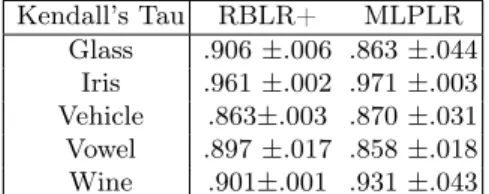
appro-Kendall’s Tau RBLR+ MLPLR Glass .906 ±.006 .863 ±.044 Iris .961 ±.002 .971 ±.003 Vehicle .863±.003 .870 ±.031 Vowel .897 ±.017 .858 ±.018 Wine .901±.001 .931 ±.043

Table 4. Performance of RBLR+, MLPLR in terms of Kendall’s tau (mean and standard deviation)

Spearman’s Rank RBLR+ MLPLR Glass .928 ±.005 .890 ±.046 Iris .971 ±.001 .977±.025 Vehicle .891 ±.003 .896±.025 Vowel .945 ±.012 .924±.013 Wine .919±.011 .948 ±.032

Table 5. Performance of RBLR+, MLPLR in terms of Spearman’s rank (mean and standard deviation)

using this kind of model, the user could be invited to analyze rules that are activated for a given query, i.e. some instance profile or a specific preference rela-tion between pairs of labels. The activated rules show which scenarios of cause-effect relationships match the considered query. For example, suppose that this following rule is obtained: IF[(q2 ≥ 2.4) ∧ (q3 ≤

1.9)]THEN(λ2 λ3). This rule not only gives a

pre-diction on the preference relation between labels λ2

and λ3, but it can also serve to argument the

recom-mendation (in this case the reason why λ2  λ3).

Moreover, this rule could also be used to select a specific feature vector (e.g. a specific user’s profile): which kind of input does verify this preference rela-tion? In other words, by knowing that λ2 λ3holds

whenever [(q2≥ 2.4) ∧ (q3≤ 1.9)], one could activate

a query to search a specific group (i.e. a specific tar-get audience) having [(q2 ≥ 2.4) ∧ (q3 ≤ 1.9)]. Such

a kind of strategy could be useful, for example, in marketing and advertising for reaching target mar-kets. Finally, the approach presented in this paper is very competitive compared to other existing meth-ods in terms of prediction accuracy. There are several directions for future work in order to improve the approach discussed w.r.t. computational complexity and efficiency. On the other hand, other possibilities could be investigated with regard to the generation of final rankings.

References

2. Greco, S., Matarazzo, B., Słowiński, R. and Stefanowski, J.: An algorithm for induction of de-cision rules consistent with dominance principle, in W. Ziarko, Y. Yao (eds.): Rough Sets and Current Trends in Computing, LNAI 2005, Springer, Berlin, pp. 304-313, (2001).

3. Har-Peled, S., Roth, D. and Zimak, D., Con-straint classification for multiclass classificatin and ranking in Advances in Neural Information Process-ing Systems, pp. 785-792, (2002).

4. Hüllermeier, E., Fürnkranz, J., Cheng, W. and Brinker, K.: Label Ranking by learning pairwise pref-erence. Artif. Intell. 172 (16-17), 1897-1916, (2008).

5. Cheng, W., Hühn, J., Hüllermeier, E.: Decision Tree and Instance-Based Learning for Labele Rank-ing. Proc. ICML-09, International Conference on Ma-chine Learning. Montreal, Canada, (2009).

6. Fürnkranz, J., and Hüllermeier, E., (eds.): Pref-erence Learning, Springer-Verlag, 2010.

7. Gärtner, T., Vembu, S.: Label Ranking Al-gorithms: A Survey. In Johannes Fürnkranz, Eyke Hüllermeier, editor(s), Preference Learning, Springer-Verlag, (2010).

8. Duda, R. O., Hart, P. E., and Stork D. G.: Pat-tern Recognition. John Wiley Sons, (2000).

9. Witten, I. H., Frank, E.: Data Mining: Practical Machine Learning Tools and Techniques. Published by Morgan Kaufmann, (2011).

10. Tan, PN., Steinbach, M. and Kumar, V., Intro-duction to Data Mining. Published by Addison Wes-ley Longman, (2006).

12. Elisseeff, A., Weston, J.: A kernel method for multi-labelled classification. In Advances in Neural Information Processing Systems 14, (2001).

13. Błaszczyński, J., Słowiński, R. and Szeląg, M.: Sequential Covering Rule Induction Algorithm for Variable Consistency Rough Set Approaches. In-formation Sciences, 181, 987-1002, (2011).

14. Błaszczyński, J., Greco, S., Słowiński, R. and Szeląg, M.: Monotonic variable consistency rough set approaches. International Journal of Approximate Reasoning, 50, 979999, (2009).

15. Błaszczyński, J., Greco, S. and Słowiński, R.: Multi-criteria classification - a new scheme for ap-plication of dominance-based decision rules. Euro-pean Journal of Operational Research, 181, 10301044, (2007).

16. Doumpos, M., Zopounidis, C.: Multicriteria Decision Aid Classification Methods. Applied Opti-mization, Volume 73, 15-38, (2004).

17. Jerzy, W., Grzymala-Busse: Rough Sets and Intelligent Systems Paradigms Lecture Notes in Com-puter Science, Volume 4585/2007, 12-21, (2007).

18. Han, J., Kamber, M.: Data Mining: Concepts and Techniques, Morgan Kaufmann, San Francisco, CA, (2006).

19. Vincke, Ph.: "L’aide Multicritère à la décision" Editions de l’ULB - Ellipses (1988).

20. Jacquet-Lagreze, E., Siskos, Y.: Preference disaggregation: 20 years of MCDA experience. EJOR 130, 233-245, (2001).

21. Sá, C. et al. Mining Association Rules for Label Ranking. Proceeding PAKDD’11 Proceedings of the 15th Pacific-Asia conference on Advances in

knowledge discovery and data mining - Volume Part II, (2011).

22. Bouyssou, D. Ranking methods based on val-ued preference relations: a characterization of the net flow method, European Journal of Operational Re-search, 60, 61-68, 1992.

23. Greco, S., Matarazzo, B., Słowiński, R.: Rough sets theory for multicriteria decision analysis, Euro-pean Journal of Operational Research, vol 129 (2001), pp. 1-47.

24. Diaconis, P., Graham, R. L.: Spearmans footrule as a measure of disarray, Journal of the Royal Statistical Society, Series B (Methodological), 39 (1977). 262-268.

25. Schapire, R.E.; Singer, Y.: Improved boosting algorithms using confidence-rated predictions. Pro-ceedings of the Eleventh Annual Conference on Com-putational Learning Theory (Madison, WI, 1998), 8091 (electronic), ACM, New York, 1998.

26. Lin, H., Li, L. (2012): Reduction from cost-sensitive ordinal ranking to weighted binary classifi-cation. Neural Computation, 24, 13291367.

27. Hung, M.S., Hu, M.Y., Shanker, M.S., Patuwo B.E.: Estimating Posterior Probabilities In Classifica-tion Problems With Neural Networks. InternaClassifica-tional Journal of Computational Intelligence and Organiza-tions, 1(1), 49-60, 199.

28. Cybenko, G.: Approximation by superposi-tions of a sigmoidal function. Mathematics of Con-trol, Signals and Systems, 2:303314, 1989.

29. Funahashi, K.I.: On the approximate realiza-tion of continuous mappings by neural networks. Neu-ral Networks, 2:183192, 1989.