Added value of far-infrared radiometry
for remote sensing of ice clouds
Quentin Libois1 and Jean-Pierre Blanchet1
1Department of Earth and Atmospheric Sciences, Université du Québec à Montréal, Montréal, Québec, Canada
Abstract
Several cloud retrieval algorithms based on satellite observations in the infrared have been developed in the last decades. However, these observations only cover the midinfrared (MIR,𝜆 < 15 μm) part of the spectrum, and none are available in the far-infrared (FIR,𝜆≥15 μm). Using the optimal estimation method, we show that adding a few FIR channels to existing spaceborne radiometers would significantly improve their ability to retrieve ice cloud radiative properties. For clouds encountered in the polar regions and the upper troposphere, where the atmosphere is sufficiently transparent in the FIR, using FIR channels would reduce by more than 50% the uncertainties on retrieved values of optical thickness, effective particle diameter, and cloud top altitude. Notably, this would extend the range of applicability of current retrieval methods to the polar regions and to clouds with large optical thickness, where MIR algorithms perform poorly. The high performance of solar reflection-based algorithms would thus be reached in nighttime conditions. Since the sensitivity of ice cloud thermal emission to effective particle diameter is approximately 5 times larger in the FIR than in the MIR, using FIR observations is a promising venue for studying ice cloud microphysics and precipitation processes. This is highly relevant for cirrus clouds and convective towers. This is also essential to study precipitation in the driest regions of the atmosphere, where strong feedbacks are at play between clouds and water vapor. The deployment in the near future of a FIR spaceborne radiometer is technologically feasible and should be strongly supported.Plain Language Summary
The size of ice cloud particles can be estimated from space by measuring the infrared emission of ice clouds. However, this method no longer works when clouds are too thick or when particles are too large, although such clouds are encountered in many regions of the Earth and are critical for the Earth’s climate. Using new sensors that measure cloud emission at longer wavelengths, in the so-called far-infrared region, would extend the potential of satellite observations to thick clouds, to clouds made of larger particles, and to clouds found in the polar regions which are very poorly known. These new sensors have become available in the last years, but none is deployed in space so far. We show that a satellite equipped with a few channels in the far-infrared would greatly increase our capacity to observe ice clouds. This is promising for our understanding of cloud microphysics and precipitation in general, and for studying the water cycle in the polar regions in particular. For these reasons, it is highly recommended to deploy a far-infrared radiometer in space.1. Introduction
Passive satellite observations have been extensively used to retrieve ice cloud radiative properties from space [e.g., Inoue, 1985; King et al., 1992; Platnick et al., 2003]. Generally, the quantities of interest are cloud optical thickness𝜏, effective particle diameter deff, and cloud boundaries altitudes. Contrary to active sensors such as CALIPSO [Winker et al., 2003] and CloudSat [Stephens et al., 2002] that only measure cross sections of cloud properties, passive sensors often allow imaging, which is very valuable to investigate the horizontal structure of clouds. A wide range of cloud retrieval methods have been developed, which generally take advantage of the strong variations of the ice refractive index throughout the solar spectrum and the infrared (IR) range. Methods based on solar reflection by clouds [e.g., Nakajima and King, 1990; King et al., 2004] are efficient for optically thick clouds but limited to daytime conditions. Methods based on cloud IR signature are efficient for optically thinner clouds but are limited for optical thickness greater than about five [e.g., Iwabuchi et al., 2014]. The IR methods have the advantage of being applicable indifferently for daytime and nightime, which ensures consistency of the retrieval independently of solar illumination conditions. The original IR methods
RESEARCH ARTICLE
10.1002/2016JD026423 Key Points:
• Ice cloud remote sensing would be greatly improved by adding far-infrared channels to existing midinfrared spaceborne radiometers • Far-infrared radiometry is well suited
to study ice clouds in the polar regions and upper troposphere • Using far-infrared radiometry extends
current infrared capabilities to large optical thickness and large cloud particles Supporting Information: • Supporting Information S1 • Table S1 • Table S2 • Table S3 Correspondence to: Q. Libois, [email protected] Citation:
Libois, Q., and J.-P. Blanchet (2017), Added value of far-infrared radiometry for remote sensing of ice clouds, J.
Geophys. Res. Atmos., 122, 6541–6564,
doi:10.1002/2016JD026423.
Received 23 DEC 2016 Accepted 3 JUN 2017
Accepted article online 9 JUN 2017 Published online 29 JUN 2017
©2017. American Geophysical Union. All Rights Reserved.
were based on the split window technique [Inoue, 1985], which consists of measuring the atmosphere bright-ness temperature in two channels having distinct sensitivities to cloud properties. Those channels were generally chosen around 11 and 12 μm, ice being much less absorbing at 11 μm than at 12 μm. Later on, the addition of supplementary channels allowed to better constrain cloud properties [e.g., Baum et al., 1994; Wei
et al., 2004; Yue and Liou, 2009; Wang et al., 2011, 2013]. These methods are mostly based on look-up-table
approaches, and retrievals are obtained by minimizing the root-mean-square deviation between the observa-tions and tabulated values. More recently, a number of algorithms based on the optimal estimation method [Rodgers, 2000] were proposed [Cooper et al., 2006; Iwabuchi et al., 2014; Wang et al., 2016a]. Such methods use all available channels to find the most likely state of a cloud. They also provide a rigorous estimation of the uncertainties associated to the retrievals.
The present study is based on the optimal estimation method and focuses on IR techniques, because those can be used at night. This is critical in the study of clouds during the polar night, a central topic of our research. Current IR retrieval methods are not appropriate in the study of optically thick clouds (𝜏 > 10) and clouds made of large particles (deff≳ 80 μm) [Merrelli, 2012; Wang et al., 2016b]. Such methods are also not suitable for the polar regions [Liu et al., 2010], due to the low thermal contrast between the surface and clouds and because the low thermal emission of these cold areas generally results in a low signal-to-noise ratio. Those limitations are essentially due to the inherent single-scattering properties of ice particles in the midinfrared (MIR,𝜆 < 15 μm), in which spaceborne radiometers such as Moderate Resolution Imaging Spectroradiometer (MODIS) [King
et al., 1992], Atmospheric Infrared Sounder (AIRS) [Aumann et al., 2003], or Advanced Very High Resolution
Radiometer (AVHRR) [Wang and Key, 2005] take their measurements. Yang et al. [2003] have shown that using well-chosen far-infrared (FIR,𝜆 ≥ 15 μm) hyperspectral channels could allow to retrieve effective particle diameter up to 100 μm, even in the case of optically thick clouds. This was confirmed by Merrelli and Turner [2013] who showed that the added value of FIR hyperspectral measurements is maximum for thick clouds and for large particles. FIR observations thus have the potential of observations performed in the solar spectrum, without their limitations.
Despite the acknowledged potential of FIR radiometry for retrieving ice cloud properties [e.g., Baran, 2007;
Merrelli, 2012; Palchetti et al., 2016a], no satellite observations of the Earth’s atmosphere were performed in
this spectral range since the Meteor satellite program in the late 1970s [Spankuch and Döhler, 1985]. The devel-opment of FIR spectrometers has been hindered for several reasons: (1) radiometric responsivity of existing sensors is much less in the FIR than in the MIR; (2) observations from the ground are in most locations useless since the atmosphere is essentially opaque in the FIR; (3) hyperspectral instruments in the MIR, such as AIRS or Infrared Atmospheric Sounding Interferometer (IASI) [Blumstein et al., 2004], already contain much informa-tion about the atmosphere. There has been in the last decade a renewed interest for satellite missions in the FIR, though, mainly fostered by the availability of new technologies based on uncooled thermal sensors such as thermopiles [McCleese et al., 2007], pyroelectrics [Palchetti et al., 2006], and microbolometers [Ngo Phong
et al., 2015]. Such sensors, when coated with gold black, have sufficient sensitivities and are easier to deploy
in space than cooled systems. The CLARREO project [Wielicki et al., 2013], for instance, aims at measuring the spectrally resolved emission spectrum of Earth up to 100 μm. However, the current radiometric resolution in the FIR (10 K) is too low to observe clouds at short time scales. Instead, the instrument aims at providing very accurate large-scale averages of the Earth’s radiative budget. The REFIR project [Palchetti et al., 2006], which has been recently renamed FORUM [Palchetti et al., 2016b], also intends to measure the FIR emission of the Earth, but is not specifically focused on ice cloud observation. These two projects, that are based on Fourier transform interferometry (FTIR), are ambitious and face budget issues, making their future still uncertain. Given that only a few channels (approximately five) contain the bulk of the information in most cloud retrieval algorithms [e.g., L’Ecuyer et al., 2006; Wang et al., 2016a], such high spectral resolution is not necessary for the specific application of cloud retrieval. As a consequence, an alternative resides in using narrow band radiometers rather than hyperspectral instruments. Such instruments can be more affordable, more robust, and less complex than FTIR systems that require high-precision optics. Radiometers essentially trade spectral resolution for radiometric resolution. This is the route chosen for the TICFIRE project (Thin Ice Clouds in the Far-InfraRed Experiment) [Blanchet et al., 2011; Libois et al., 2016a], which consists of a filter wheel IR imager with channels spanning the whole IR range from 8 to 50 μm. This mission, currently under review at the
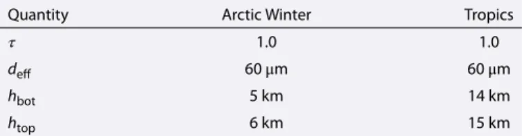
Table 1. Cloud Characteristics for the Two Reference Cases
Quantity Arctic Winter Tropics
𝜏 1.0 1.0
deff 60μm 60μm
hbot 5 km 14 km
htop 6 km 15 km
Canadian Space Agency, will be dedi-cated to the observation of ice clouds in the polar regions and can be viewed as a FIR extension of MODIS.
The present study investigates the potential of FIR radiometry for ice cloud radiative properties retrieval. For this, the information content of FIR radiances for a variety of cloudy scenes is estimated in the framework of the optimal estimation method. This work follows the method implemented by Wang et al. [2016a] and Iwabuchi et al. [2016] for MODIS observations but extends these studies to the case of FIR channels. Of particular importance is the estimation of effective particle diameter and the distinction between precipitating and nonprecipitating clouds. A special focus is thus put on uncertainties related to effective particle diameter retrievals and on the capacity to accurately estimate particle size for large particles. In the driest regions of the troposphere, that is, the polar regions and the near-tropopause, precipitation can result in the dehydration of the atmosphere [Curry et al., 1995; Jensen et al., 1996]. This can significantly alter the radiative budget, which is essentially driven by the natural greenhouse effect of water vapor [Blanchet and
Girard, 1995]. Hence, cloud effective particle diameter is a critical quantity that affects the radiative budget of
the Earth [e.g., Stephens et al., 2002]. Improving existing cloud retrieval algorithms could complement active technologies which provide valuable insight into clouds microphysics, formation, and evolution [e.g., Austin
et al., 2009; Grenier et al., 2009; Kayetha and Collins, 2016]. After providing a physical insight on the potential of
FIR radiometry for studying ice clouds, section 2 provides details on the optimal estimation framework and on the synthetic satellite instrument used in this paper. In section 3, the information content of FIR observations is computed for two representative cases, namely a polar ice cloud and a tropical ice cloud. The added value of FIR is discussed in section 4, where leads for future work and recommendations for designing a spaceborne FIR radiometer are also given.
2. Motivation and Methods
In this section, the theoretical framework used to quantify the information content of FIR radiances for cloud properties retrieval is detailed. It is based on the optimal estimation method [Rodgers, 2000] and follows the approach of Wang et al. [2016a] and Iwabuchi et al. [2016]. Two types of ice clouds are studied in detail: a polar ice cloud and a tropical ice cloud. Since no spaceborne FIR radiometer exists so far, a synthetic instrument is used, whose characteristics are mainly based on those of the Far-InfraRed Radiometer (FIRR) [Libois et al., 2016a], which is a breadboard for the TICFIRE mission.
2.1. Atmospheric Profiles
The two types of clouds considered in this study are supposed to encompass most climatically relevant ice clouds encountered on Earth: a high-altitude ice cloud in a tropical atmosphere, which can be either a cirrus cloud or the anvil of a convective cloud, and a ubiquitous tropospheric ice cloud during Arctic winter. Both clouds are single layer and assumed homogeneous. The tropical cloud is located just beneath the trop-ical tropopause, between 14 and 15 km, while the polar cloud extends from 5 to 6 km altitudes consistent with the CALIPSO observations reported by Haladay and Stephens [2009] in the tropics and Grenier et al. [2009] in the Arctic. The atmosphere within the clouds is saturated. In the reference cases, those clouds have an optical thickness of 1.0 and a effective particle diameter of 60 μm, corresponding to a modified-gamma distribution with effective variance 0.1 [Petty and Huang, 2011] of severely roughened column aggregates [Yang et al., 2013]. The same distribution is assumed in the Collection 6 MODIS cloud product [Holz et al., 2016]. The characteristics of these reference cases are summarized in Table 1. The vertical profiles of temperature and water vapor mixing ratio for both atmospheres were computed from an average of 18 radiosondes taken from the IGRA database (ftp://ftp.ncdc.noaa.gov/pub/data/igra/). For the tropical profile, six radiosondes measured between 1 January 2015 and 1 November 2016 were randomly taken from each of the following stations: Abidjan, Corozal Oeste, and Piarco International Airport. The Arctic winter profile was computed from radio soundings measured in January or February of 2015 or 2016 at Alert, Eureka, and Resolute Bay. This profile is meant to be representative of typical winter conditions in the Canadian Archipelago. Both profiles are shown in Figure 1.
Figure 1. Atmospheric profiles for the Arctic winter and tropical
reference cases. The positions of the ice clouds are indicated by the horizontal shaded area.
2.2. Instrument Characteristics
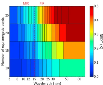
Contrary to the works of Wang et al. [2016a] and Iwabuchi et al. [2016] that were dedi-cated to MODIS, here we do not investigate the characteristics of a particular instru-ment but rather explore the potential of a synthetic spaceborne FIR radiometer. The instrument is characterized by its number of channels and by its noise equivalent radiance (NER). For the sake of simplicity, the bands are contiguous and cover the range 6–100 μm, because at shorter wave-lengths the contribution of solar radiation cannot be neglected in daytime conditions. The spectral responses are rectangular and the bandwidths such that all bands receive the same amount of radiance at the top of atmosphere (TOA) for the Arctic winter reference case. This equienergetic partition of the channels implies that FIR bands are much wider than MIR bands (Figure 2). The reference configuration of the instrument is 10 bands, and the NER is assumed the same for each channel, equal to 0.01 W m−2sr−1. This is consistent with a thermal sensor coated with gold black which has spectrally flat absorbance through the whole IR range [e.g., Ngo Phong
et al., 2015], and with the absence of significant spectral differences in the transmittance along the optical
path. Such characteristics are expected for a grating-based or filter wheel-based radiometer. The radiomet-ric resolution is defined in terms of NER rather than in terms of noise equivalent delta temperature (NEDT) to work at the sensor level. NEDT is helpful in comparing to actual temperature measurements, but it can be misleading as it depends on the temperature of the considered scene. Also, with this choice, increasing the number of bands clearly results in a decrease of the signal-to-noise ratio, which is easily understood because
Figure 2. NEDT in each spectral channel as a function of total number of
equienergetic bands, for a blackbody at 250 K. The NER is assumed spectrally constant and equals 0.01 W m−2sr−1.
the sensor NER remains constant, inde-pendently of the channels configura-tion. In the case of gratings, for instance, an increase of the spectral resolution is generally obtained at the expanse of radiometric resolution. For the sake of comparison with other studies, though, Figure 2 shows the NEDT correspond-ing to an NER of 0.01 W m−2 sr−1 for different instrument configurations. The 20 band configuration is such that MIR NEDT is less than 0.2 K, which is similar to MODIS NEDT at 250 K. This suggests that the microbolometer-based radiometer could perform as well as MODIS sensor, except that its spectral coverage would be extended throughout the FIR. In addition to this synthetic instrument, the method is applied to MODIS and to the TICFIRE instrument in section 4.1.
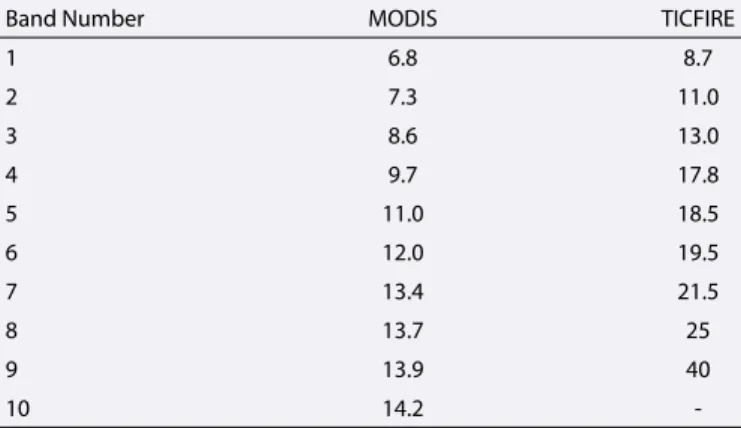
Table 2. Spectral Bands of MODIS and TICFIRE Used in This Studya
Band Number MODIS TICFIRE
1 6.8 8.7 2 7.3 11.0 3 8.6 13.0 4 9.7 17.8 5 11.0 18.5 6 12.0 19.5 7 13.4 21.5 8 13.7 25 9 13.9 40 10 14.2
-aThe values indicate the central wavelengths inμm.
To this end, the 10 MODIS IR channels analyzed by Iwabuchi et al. [2016] are used, and the NER for each channel is computed from Xiong et al. [2009]. The nine TICFIRE channels are defined as those of the FIRR prototype [Libois
et al., 2016a, Figure 2a] and cover
the range 8—50 μm, and the NER is assumed to be 0.01 W m−2 sr−1 in each channel. The spectral character-istics of all these channels are detailed in Table 2. The FIRR is very similar to the Mars Climate Sounder [McCleese
et al., 2007] in terms of spectral
cover-age, and preliminary airborne and in situ measurements have highlighted the performances of this device, mak-ing it a realistic spaceborne instrument within the next years [Libois et al., 2016b]. The noise levels used for MODIS and TICFIRE remain constant throughout the paper.
2.3. Physical Motivation
Most IR cloud retrieval algorithms take advantage of spectral variations of ice and water refractive index. Figure 3a shows the imaginary parts of ice and water refractive indices. It highlights the much stronger absorp-tion at 12 μm compared to 8 μm, which explains why in many algorithms a channel around 8 μm is used along with a channel around 12 μm. In the FIR, ice shows a unique behavior compared to liquid water. Ice absorption indeed exhibits a significant minimum around 23 μm. At this minimum, the imaginary index miis 2.7 × 10⁻², which is less than the value at 8.7 μm (3.7 × 10⁻²). Since the ice absorption coefficient is defined as
ki= 4𝜋mi∕𝜆, the latter is nearly 3 times lower at 23 μm than at 8.7 μm. It is also 30% less than at 3.7 μm, a crit-ical channel to study optcrit-ically thick clouds that is however affected by solar radiation in daytime conditions [Nakajima and King, 1990; Platnick et al., 2003]. The ice refractive index spectral features determine the spectral dependence of the extinction coefficient and single-scattering albedo of ice crystals (Figures 3b and 3c). The reduced size parameter (x =𝜋deff∕𝜆) for wavelengths beyond 30 μm is responsible for a large sensitivity of the extinction efficiency and single-scattering albedo to effective diameter compared to the MIR. This makes FIR more appropriate than MIR for studying large cloud particles. In addition, the single-scattering albedo is relatively high around 23 μm and remains well above 0.5 for large particles. As a consequence, a significant amount of multiple scattering occurs in this range so that optically thick ice clouds are partly reflective and have an emissivity below 1. This drastically increases the sensitivity of emitted radiance to the effective parti-cle diameter [Yang et al., 2003], contrary to the perfect blackbody behavior observed in the MIR that hinders any information about cloud particle size. Such spectroscopic characteristic is favorable for studying cloud microphysics at the top of optically thick convective towers, for instance, where standard IR algorithms show poor performance. To some extent, the FIR contains similar information to MODIS channel centered at 3.8 μm used by Wang et al. [2016a], with the advantage of being unaffected by solar radiation. Note also that ice cloud optical thickness can be significantly different at 10.6, 12, 23, or 35 μm (Figure 3b). For instance, a cloud with effective particle diameter of 30 μm becomes opaque (i.e., optical thickness equals 5) at visible optical depth of 6.25 at 10.6 μm, 4 at 23 μm, and 7.63 at 35 μm. Mention of large optical thickness in the following should be considered relative to the wavelength of interest.
As shown above, the single-scattering properties of ice clouds are more sensitive to effective particle diam-eter in the FIR than in the MIR. The spectral signature of ice clouds at TOA does not depend only on their single-scattering properties, though. It also depends on the transparency of the atmosphere and on the total amount of radiation reaching the instrument. From the ground, the atmosphere is often opaque in the FIR range due to strong absorption by water vapor, so that FIR observations are generally disadvantaged com-pared to MIR observations. Largely for that reason, most studies dedicated to FIR radiation were taken in dry, cold, or elevated locations [e.g., Turner and Mlawer, 2010; Shi et al., 2016]. On the contrary, from a satel-lite perspective, clouds can be observed in the FIR if the atmosphere above them is sufficiently transparent.
Figure 3. (a) Imaginary part of ice and water refractive indices in the range 3.5–50μm. Spectral variations of the (b) extinction coefficient and (c) single-scattering albedo for a distribution of severely roughened column aggregates from the database of Yang et al. [2013].
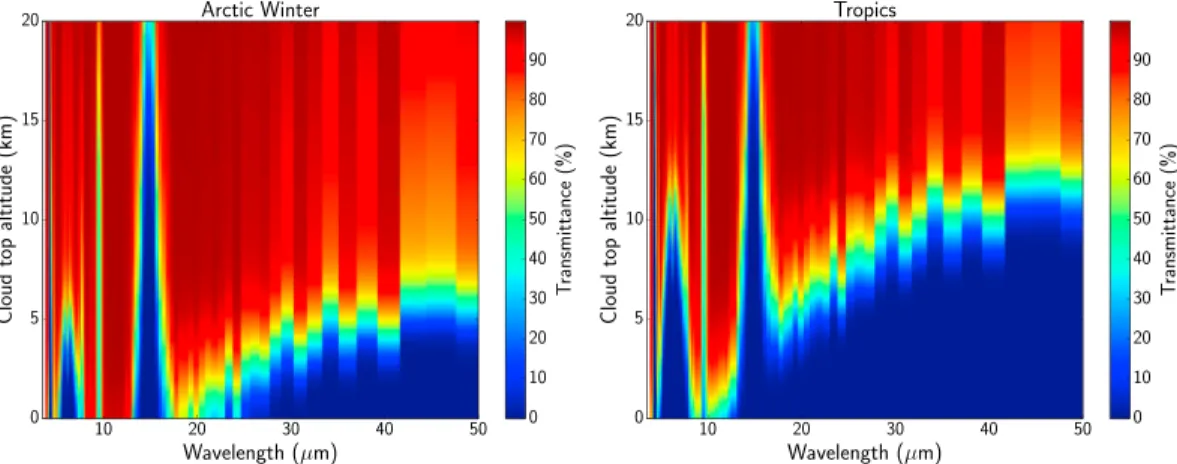
Figure 4 shows the transmittance of the atmosphere above the reference clouds as a function of cloud top alti-tude. It shows that an ice cloud can be well observed from space up to 50 μm as soon as its top is above 5 km (10 km) for Arctic winter (tropical) conditions. These conditions are highly relevant because thin ice clouds encountered in the polar regions and tropical cirrus and convective towers often satisfy those conditions. It also shows that FIR offers an effective profiling capability throughout most of the atmosphere, by masking lower atmospheric layers and shielding the surface with increasing wavelengths in the range 17–40 μm.
2.4. Optimal Estimation Framework 2.4.1. Theoretical Framework
Generally speaking, the information content of a radiance measurement depends on its sensitivity to changes in cloud properties, on the uncertainties regarding the atmospheric state, the cloud particle size distribution and shape, and on the instrumental error. The optimal estimation method [Rodgers, 2000] accounts properly for all these contributions and has been used to assess the information content of various IR instruments such as MODIS [L’Ecuyer et al., 2006] and IASI [Rabier et al., 2002]. Since the present paper focuses on cloud radiative properties, the state vector to be retrieved only includes cloud properties. Following Wang et al. [2016a], only single-layer homogeneous clouds are considered, and the state parameter consists of the cloud top altitude
h, the optical thickness𝜏, and the effective particle diameter deff. The cloud is assumed to be 1 km thick. All other atmospheric properties contribute to the measurement error, implying that the atmospheric state must be provided by another satellite (e.g., AIRS) or reanalysis product (e.g., ERA-Interim) [Dee et al., 2011]. Note that for hyperspectral observations, all atmospheric properties can be included in the state parameter [e.g., Merrelli and Turner, 2013].
Figure 4. Simulated spectral atmospheric transmittance between the top of a cloud and the TOA as a function of cloud
top altitude, for Arctic winter and tropical conditions. The simulations were performed at 15 cm−1spectral resolution.
The optimal estimation framework can be written as follows:
y = F(xt, Tst, 𝝐ts, Tt, RHt, Ht)+𝝐obs, (1) where y is the observation vector, F the forward model that returns the TOA radiances as a function of all atmo-spheric information, and𝜖obsthe observation error. The superscript t indicates the true state, which means that the forward model is assumed perfect. This is consistent with the results of Wang et al. [2016a] who showed that model errors are much smaller than other contributions. Besides the state vector x, the simulated TOA radiance depends on surface temperature Ts, surface spectral emissivity𝝐s, temperature and relative humidity profiles T and RH, and ice habit H including actual habit and particle size distribution. Since the true param-eters are unknown, the simulated radiance computed from a best estimate of the atmospheric state deviates from the true radiance, so that equation (1) can be rewritten as
y = F(xt, T
s, 𝜖s, T, RH, H )
+𝜖Ts+𝜖𝝐s+𝜖T+𝜖RH+𝜖H+𝜖obs, (2)
y = F(xt, p) + 𝝐y, (3)
where the measurement error𝝐yis the sum of errors𝜖i = 𝜕F 𝜕pi
(
pi− pti )
,𝜖H, and𝜖obs, and p the parameter vector including all ancillary parameters pi. The optimal estimation method aims at determining the posterior distribution of xtgiven an a priori on x and a set of observations. The quantity to be retrieved is thus P(xt|y). According to Bayes’ theorem,
P(xt|y) =P(y|xt)P(xt)
P(y) . (4)
For the sake of simplicity, it is assumed that all probability density functions are Gaussian. Although this is a strong assumption, it is very widely used, especially in data assimilation, due to the resulting easiness of implementation. In this case,
ln(P(y|xt))=[y − F(xt, p)]⊤S−1 y [ y − F(xt, p)]+ c 1, (5) ln(P(xt))=[xt− xa]⊤S−1 a [ xt− xa]+ c 2, (6)
where Syis the error covariance matrix corresponding to the errors𝝐y, xathe a priori state parameter, and Sa its associated error covariance, and the subscript T indicates transposition. Sais such that the a priori uncer-tainties on h is 4 km, and𝜏 and deffare known within a factor of 10 and 5, respectively; c1and c2are constants. From equation (4), ln(P(xt|y))=[y − F(xt, p)]⊤S−1 y [ y − F(xt, p)]+[xt− xa]⊤S−1 a [ xt− xa]+ c 3. (7)
It can be shown [Rodgers, 2000] that the posterior distribution P(xt|y) is then defined as a multivariate Gaussian distribution with mean xpand error covariance matrix S
psuch that ln(P(xt|y))=[xt− xp]⊤S−1 p [ xt− xp]+ c 0, (8) Sp= ( S−1 a + K⊤xS−1y Kx )−1 . (9)
The matrix Kxcontains the derivatives of the TOA radiance with regard to the state parameters, also called the Jacobians: Kx= [ 𝜕F 𝜕h, 𝜕 F 𝜕𝜏, 𝜕 F 𝜕deff ] . (10)
The state xoptthat maximizes P(xt|y) is the maximum likelihood estimation. For retrieval applications it can be estimated using the Gauss-Newton algorithm [Rodgers, 2000]. This iterative method is such that the state xn+1at step n+1 is determined from the state xnat step n by
xn+1= xa+ ( S−1 a + K T nS −1 y,nKn )−1 KT nS −1 y,n [ y − F(xn) + Kn(xn− xa)], (11) where the Jacobians and error covariance matrices are computed at each step n.
2.4.2. Measurement Error Contributions
In this study, three independent sources of errors are considered: (1) observation error, (2) uncertainties on the surface and atmospheric states, and (3) uncertainties on crystal habit and particle size distribution. All the error sources are assumed independent, and the global error covariance matrix Syis simply the sum of all the individual contributions. Uncertainties in trace gases concentrations, though potentially critical for channels overlapping CO2or O3absorption bands, are not considered here. All radiative transfer calculations are per-formed with MODTRAN v.5.4 [Berk et al., 2005] using the correlated-k method. Multiple scattering is accounted for using DISORT [Stamnes et al., 1988] with 16 streams. The water vapor continuum is computed from the MT-CKD 2.5 parameterization [Clough et al., 2005]. The spectral surface emissivities are taken from Feldman
et al. [2014]. For the Arctic winter case, it is assumed that the surface is snow covered, while for the tropical
case, it is ocean water.
For the observation error, the instrument NER is assumed similar in each band, equal to 0.01 W m−2 sr−1. This is consistent with the laboratory characterization of the FIRR [Libois et al., 2016a] when averaging the signal over a 2-D array of uncooled microbolometers. Although such NER is not yet achieved for a FIR imaging system, it is expected that improved optical and electronic design should allow to meet this target within a few years. The absence of any window on the optical path in space will also be beneficial to the response of the instrument, contrary to ground operation in which the FIRR detector works under vacuum in a sealed package. Observation errors in distinct channels are assumed uncorrelated, so that the error covariance matrix Sobsis diagonal.
Uncertainties on surface emissivity, surface skin temperature, and temperature and humidity profiles, alto-gether referred to as ancillary parameters, also affect the quality of the retrieval. Here we assumed that the surface emissivity uncertainties in each band are uncorrelated and equal to 0.01. Such errors correspond to the imperfect knowledge of surface emissivity in the FIR, not to a mischaracterization of the surface which would result in larger and correlated errors [Feldman et al., 2014]. This implies that such values hold only when the type of surface is well known. Surface temperature uncertainty is taken as 0.5 K. The errors on the temperature and humidity profiles are 1 K and 15% at each level. These errors are vertically correlated in an exponential way such that correlation vanishes at 1 km distance. Such values, also used by Wang et al. [2016a], are consistent with the accuracy of state-of-the art reanalysis products or IR sounders atmospheric products. The prior and measurement uncertainties used in the study are summarized in Table 3. The case of larger uncertainties for the atmospheric and surface parameters, which might be more realistic for the Arctic, is discussed in section 4. The derivatives of TOA radiance with respect to the ancillary parameters are computed with MODTRAN using finite differences [e.g., Garand et al., 2001] to convert the above mentioned errors into measurement errors (equation (2)). These measurement errors depend on cloud characteristics and are thus computed for each individual scene.
Studies dedicated to the MIR generally neglect the impact of particle size distribution, because it was shown to induce smaller uncertainties than crystal habit [e.g., Cooper et al., 2006]. Although this is true for the MIR,
Table 3. Uncertainties for the Prior State Parameters, for the Ancillary Parameters, and for the
Radiance Measurements Used Throughout the Studya
Quantity ln𝜏 ln deff h Ts 𝜖s T RH Radiance Uncertainty (nominal) ln 10 ln 5 4 km 0.5 K 0.01 1 K 15% 0.01 W m−2
Uncertainty (high) - - - 2 K 0.03 2 K 25%
-aThe high values are used in section 4.2.
it is not the case in the FIR where particle size distribution can have an impact similar to crystal habit [Baran, 2007]. As a consequence, it is included in the present error analysis because both habit and size distribution uncertainties can result in changes of TOA radiance close to 5% in FIR bands. To account for those uncertain-ties, several simulations were performed for various habits and size distributions. Practically, the nine habits of the database of Yang et al. [2013] are used, with the three investigated roughness parameters. Size distribu-tions are assumed to follow a modified-gamma distribution [e.g., Petty and Huang, 2011; Merrelli and Turner, 2013] with effective variances 0.1 or 0.2. For each cloud scene, 54 simulations are thus performed, and the error covariance matrix Shabis computed from these simulations.
2.4.3. Information Content
The information content of a set of observations is estimated through Shannon information content (SIC), which quantifies the entropy reduction of the state parameter resulting from the observations. Here SIC is defined as
SIC =1 2ln |||SaS
−1
p ||| . (12)
This quantity can be used to compare the information content of observations taken either with different instruments or with a particular set of channels. For instance, it has been used to select the most infor-mative channels of IASI [Rabier et al., 2002], which are currently assimilated in numerical weather forecast models or to identify the most informative channels of MODIS [Cooper et al., 2006; Wang et al., 2016a]. In addition to SIC, the retrieval uncertainty for each state parameter is defined as the square root of the diagonal elements of Sp.
3. Results
3.1. Jacobians of TOA Radiance
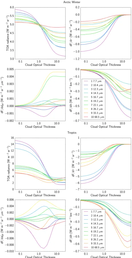
The Jacobians of TOA radiance in terms of the state parameters were computed for both Arctic and tropical atmospheres. They are shown in Figure 5 as a function of cloud optical thickness. Since the bandwidths were selected to equipartition the amount of energy available in each band for the reference Arctic winter case, the energy partition slightly varies with optical thickness. As a consequence, for large optical depth, the amount of energy available in FIR bands exceeds that available in MIR bands, because the cloud scene becomes colder and Planck emission spectrum is shifted toward the FIR. For the same reason, the energy available in FIR bands is similar for the Arctic and tropical reference cases, because FIR channels probe the higher troposphere, which temperature is similar in the Arctic and tropics. On the contrary, MIR observations are greatly advan-taged at low optical depth in the tropics because they are sensitive to the high emission of the warm surface. Fortunately, FIR observations do not suffer the disadvantage of MIR observations in cold regions. More generally, the thermal contrast between the surface and the cloud is much larger in the MIR, making MIR observations more sensitive to small changes of optical thickness in warm regions.
The most striking point in Figure 5 is the high sensitivity of FIR TOA radiance to changes in defffor the Arctic case. Indeed, while MIR sensitivity is relatively low and completely vanishes at optical thickness above 10, the sensitivity around 23 μm is much larger and increases with optical thickness. This intrinsic advantage of the FIR results from the larger sensitivity of cloud single-scattering properties to effective diameter highlighted in Figure 3. The small differences of single-scattering albedo are amplified through multiple scattering, so that the advantage increases with optical thickness. When clouds become perfectly opaque to surface radiation, their signature only comes from cloud emission. As in the MIR, thick clouds are nearly blackbody emitters; their signature is independent of deff. In the FIR, on the contrary, because clouds have emissivity less than one, their signature still carries information about particle size. This is very similar to clouds characteristics at 3.7 μm [Wang et al., 2016a] or in the visible [Nakajima and King, 1990]. For the tropical case, FIR channels are
Figure 5. Jacobians of TOA radiance with respect to cloud state parameters for the Arctic winter and tropical
atmospheres. Both clouds consist of severely roughened column aggregates with effective diameter 60μm following a modified gamma distribution with effective variance 0.1. The Arctic winter cloud is located between 5 and 6 km, and the tropical cloud is between 14 and 15 km.
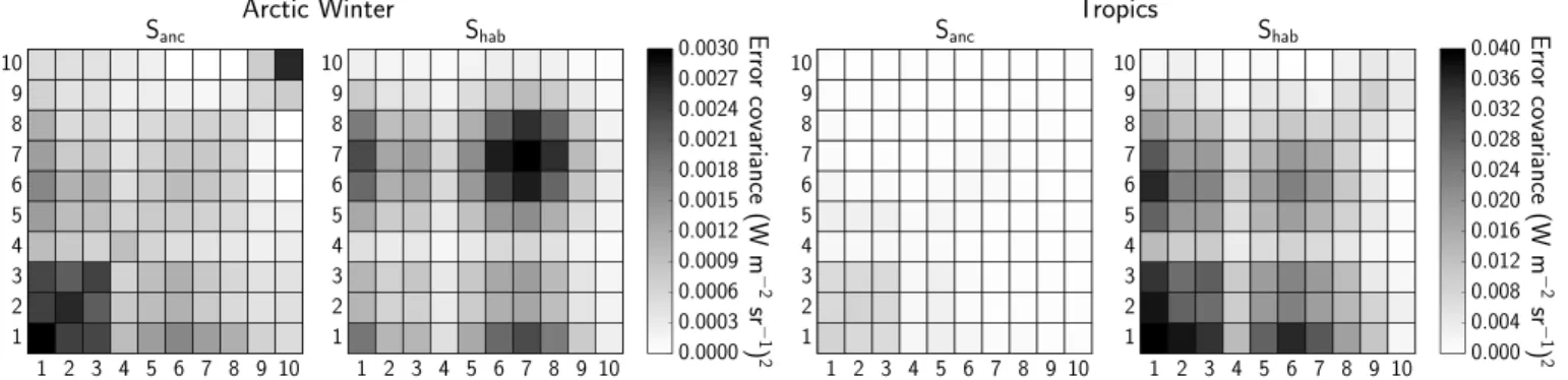
Figure 6. Error covariance matrices of the ancillary parameters (Sanc) and crystal habit (Shab) for both reference cases. The numbers correspond to the spectral bands as follows: 1: 7.7μm; 2: 10.4μm; 3: 12.3μm; 4: 14.3μm; 5: 16.7μm; 6: 19.2μm; 7: 22.1μm; 8: 26.2μm; 9: 33.3μm; 10: 68.5μm.
mainly advantaged at large optical thickness. At small optical thickness, the smaller sensitivity of MIR channels to deffis compensated by the larger thermal contrast between the surface and the extremely cold cloud. This shows that FIR observations can be extremely useful to observe cloud microphysics at the top of optically thick convective towers, for instance [Jensen et al., 1996]. Using FIR channels overall offers a way to overcome the natural limit of MIR algorithms at large optical thickness [Iwabuchi et al., 2016].
3.2. Error Covariance Matrices
The error contributions of ancillary parameters and crystal habit for the two reference cases are shown in Figure 6. Observation errors are not shown because they are much smaller. For the Arctic case, uncertainties on surface temperature and emissivity have a strong impact because the atmosphere is very transparent. They impact more MIR channels, which are more sensitive to the surface than FIR channels. FIR channels are mostly affected by water vapor uncertainties above the cloud. Crystal habit induces the largest errors in the weakly absorbing channels of the FIR, because multiple scattering amplifies small differences in single-scattering properties. This large uncertainty is nevertheless compensated by the advantageous sensitivity to deff dis-played in Figure 5. Crystal habit impact is less in the MIR, because single-scattering properties are less dependent to crystal habit. For the tropical cloud, errors on ancillary data do not impact much the global error because surface emission barely reaches the top of the atmosphere in such wet conditions, and because errors on temperature and humidity profiles below the cloud are largely attenuated by the cloud. Regarding crystal habit, its absolute impact is larger in the MIR because the amount of radiation in these bands is almost 3 times more than in the FIR (Figure 5). However, the relative uncertainty in simulated radiances due to crystal habit uncertainties remains much larger in the FIR than in the MIR.
These uncertainties are propagated to the retrieved state of the atmosphere through the optimal estima-tion method. To estimate the contribuestima-tion of each error source to the total uncertainty of the retrieved state parameters, the posterior uncertainty is first computed, accounting for all the sources and then a single source contribution is removed. The contribution of the removed source is defined as the difference. Those contri-butions are shown in Figure 7 for both reference cases. It shows that, in general, observation errors are minor, except for the determination of deffin the Arctic. More generally, observation uncertainties are more critical in the Arctic because of the lower signal-to-noise ratio. In the Arctic, h and𝜏 retrievals mainly depend on ancil-lary parameter uncertainties, while in the tropical case, ice habit is critical as well because most of the signal comes from the cloud, not from the atmosphere below.
3.3. Information Content Analysis
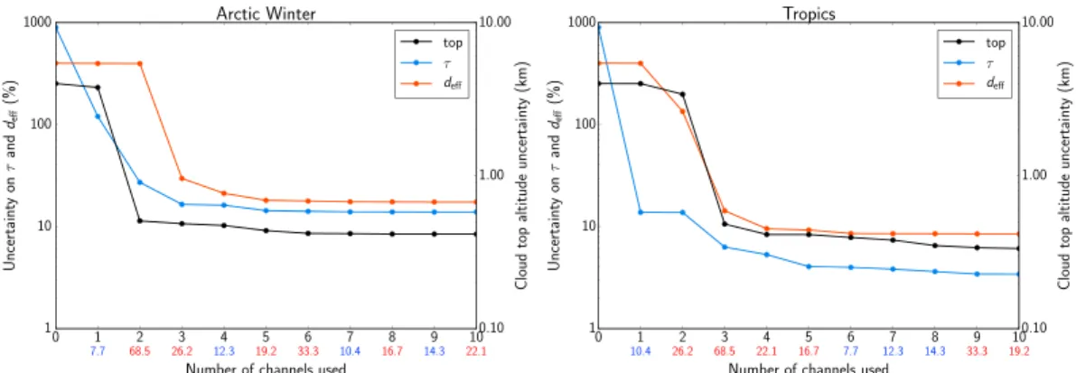
The information content of a set of observations is assessed through SIC (section 2.4.3). For a given atmo-spheric configuration, this quantity is used to select channels containing most information in a decreasing order. The first channel selected is that which contains, alone, most information. The second channel is that of the remaining channels, which when added to the first selected, adds up most of the remaining information, and so on. Each time a new channel is added, the total information content increases and the uncertainties on the state parameters decrease. Figure 8 shows the progressive decrease of the uncertainties as the num-ber of channels used increases, for the two reference cases. In both cases, the first selected channel essentially constrains the optical thickness. Thereafter only are cloud top altitude and effective particle diameter are con-strained. Interestingly, although the first channel selected is in the MIR, the next two are in the FIR. In the tropical case, channels 2 to 5 are in the FIR. It should also be noted that most information is captured with
Figure 7. Contributions of the error sources to the total posterior uncertainties, when MIR and FIR channels are used.
Each source contribution is obtained by computing the difference between the total posterior uncertainties and the uncertainties when this source is removed.
only five channels, the reduction in uncertainty beyond five channels being marginal. This is consistent with the findings of Wang et al. [2016a]. Regarding the degree of uncertainty, cloud top altitude can be estimated within about ±400 m. Optical thickness and effective diameter can be retrieved within approximately 15% to 20% error for the Arctic case, and within less than 10% error in the tropical case.
Figure 8. Decrease of state parameters uncertainties as the number of observations increases. The numbers below the
graphs indicate the central wavelengths of the selected channels. Blue refers to MIR channels while red indicates FIR channels.
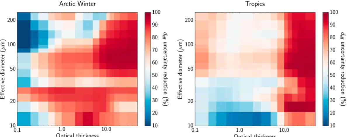
Figure 9. Uncertainties onh,𝜏, anddeffafter all channels of the 10-band synthetic radiometer have been used, for a wide range of cloud optical thickness and effective particle diameter.
These uncertainties illustrate two particular cases. To explore how they change as a function of cloud char-acteristics, the same method was applied to various combinations of cloud thickness and effective particle diameter. The resulting uncertainties are shown in Figure 9. In general, errors for the Arctic case are larger than those for the tropics. The noise level of the instrument being fixed, the signal-to-noise ratio is indeed lower in the Arctic because the emitted radiation from the colder scene is lower. The effective particle diameter retrieval performs best for optical thickness above 1 and for effective diameter up to approximately 150 μm. This is likely to extend the potential of MIR radiometry that generally performs poorly for optical thickness larger than 5 and effective diameter exceeding 100 μm. The retrievals of optical thickness are best for interme-diate optical thickness (1.0 < 𝜏 < 10) but are also very efficient in the tropics for optically thin and optically thick clouds. Cloud top altitude is very well constrained, except for very thin clouds. Errors on deffare often below 15%, making it possible to distinguish without ambiguity small particles from large particles.
Figure 10. Identification of the five most informative channels (in decreasing order of importance), when (left) cloud optical thickness or (right) effective particle
diameter are varied from the reference cases.
Figure 10 shows the five most informative channels for both reference cases, when optical thickness and effec-tive diameter are varied from the reference state. The channels 26.2 and 68.5 μm often appear in the first positions, which can be explained by the large amount of information they contain about cloud top and effec-tive diameter. In most situations it remains necessary to use at least one MIR channel because it constrains well the optical thickness in the atmospheric window. Note also that some channels have less importance and are seldom selected. This suggests that removing channels 14.3, 19.2, and 33.3 μm would not degrade the performance of the radiometer. Such considerations should be borne in mind when designing a new instrument.
4. Discussion
4.1. Added Value of FIR Observations
It was shown that FIR observations are most useful when the thermal contrast between the cloud and the surface is low, when the cloud is opaque in the MIR, and when the atmosphere above the cloud is sufficiently transparent to let cloud emission escape to TOA. The former conditions are encountered when cloud optical thickness is large or when the surface is cold. This makes FIR observations very valuable to probe polar ice clouds and optically thick high-altitude ice clouds in general. Although the potential of FIR radiometry has been shown in terms of absolute retrieval performances (Figure 9), it is worth quantifying the added value relative to MIR-only observations. To this end, the method detailed in section 3.3 was applied to a synthetic radiometer made of only the first four MIR bands of the 10-band synthetic radiometer. The relative decrease in deffuncertainty resulting from the addition of the six FIR channels is presented in Figure 11. As expected, in both Arctic and tropical cases, the largest improvement is for optical thickness beyond 10, because those are the conditions where FIR observations are most sensitive to deff, contrasting with the inherent limitations of MIR observations in such cases. In those cases, the uncertainty is reduced by more than 80%. The improve-ment is very significant for intermediate optical thickness (𝜏 = 0.5 − 5) as well, often exceeding 50%. This is particularly true for the Arctic case which is inherently disadvantaged with MIR alone due to the low radiance emitted by the cold surface. At small optical thickness, the uncertainty is barely reduced for the Arctic case. On the contrary, it is largely reduced in the tropical case because the thermal contrast between the surface and the cloud is larger, and the cloud emission in the FIR is unaltered by water vapor absorption above. This highlights the strong potential of FIR observations for studying optically very thin cirrus clouds, especially for large ice crystals (deff> 50μm). To some extent, using FIR observations adds a new retrieval capability for thick clouds and large particles in cases without reflected solar radiation.
Adding FIR channels not only reduces the uncertainties of the retrieved cloud properties but also reduces the correlations between the retrieved state variables. Table 4 shows these correlations𝜌 for both reference cases, when only MIR channels are used and when all channels are used. Adding FIR channels reduces all the correlated errors and is most useful to discriminate between h and deff.
Figure 11. Relative decrease indeffuncertainty resulting from the addition of six FIR channels to four MIR channels, for Arctic winter and tropical conditions.
So far, the obtained results are theoretical because the instrument which they refer to does not exist yet. To give it a more realistic flavor, the same method was applied to the real instruments described in section 2.2. For this, the added value of the future TICFIRE satellite was quantified with regard to MODIS (see section 2.2). Figure 12 is similar to Figure 11 except that the reference corresponds to the 10 bands of MODIS, and the full instrument corresponds to MODIS channels complemented by the nine channels of TICFIRE. The patterns for the effective particle diameter are very similar to those of Figure 11. The values are slightly lower, though, because the 10 channels of MODIS contain more information than the four MIR channels of the synthetic radiometer. The largest difference is the more limited improvement for cloud particles beyond 100 μm in the tropical case. The reductions in uncertainty for optical thickness and cloud top altitude are also shown for the Arctic case. FIR observations help constrain all cloud parameters for a large variety of cloud characteristics. They also reduce the correlated errors of the retrieved parameters (Table 4). The reductions in uncertainty for cloud top altitude and optical thickness in the tropical case are not shown since they are not as significant as in the Arctic case. These results overall highlight that adding TICFIRE observations to existing MODIS obser-vations would greatly increase the performance of cloud properties retrieval algorithms in the polar regions and also for thin cirrus and convective ice clouds in the tropics [Hong et al., 2007].
The added value of FIR observations is further illustrated in Figure 13 (similar to Figure 8), showing how using TICFIRE observations reduce the uncertainties on cloud properties for a thin and a thick Arctic cloud. It sug-gests that adding two or three FIR channels to MODIS would drastically improve cloud retrieval performance. Practically, this could be done at reasonable cost by adding such a FIR radiometer on the A-Train or Earth-CARE orbit [Illingworth et al., 2015]. Alternatively, it suggests that a compact radiometer such as TICFIRE, which covers the MIR and the FIR, could entirely replace MODIS for ice cloud monitoring.
4.2. Range of Validity of the Algorithm
All previous results are bound to the assumed uncertainties of the ancillary parameters. Those were chosen to be consistent with the work of Wang et al. [2016a] but may be optimistic, especially for the polar regions where a priori atmospheric profiles are generally poorly constrained. To estimate the sensitivity of the results to the
Table 4. Correlations Between the Retrieved State Parameters for the Two
Reference Cases, When MIR-Only or MIR and FIR Channels Are Useda
Arctic Winter Tropics MIR MIR + FIR MIR MIR + FIR
𝜌ln𝜏,ln deff −0.88 (−0.65) −0.13 (−0.02) −0.56 (−0.43) −0.41 (−0.56) 𝜌ln𝜏,h −0.97 (−0.97) −0.67 (−0.49) −0.87 (−0.60) −0.31 (−0.15) 𝜌ln deff,h 0.87 (0.67) −0.016 (0.06) 0.54 (0.30) −0.20 (−0.06)
aThe quantities in parenthesis indicate the correlated errors when
Figure 12. (top row) Relative decrease indeffuncertainty resulting from the addition of the nine TICFIRE channels to 10 MODIS channels, for Arctic winter and tropical conditions. (bottom row) Relative decrease in𝜏andhuncertainties resulting from the addition of the nine TICFIRE channels to 10 MODIS channels for the Arctic winter atmosphere.
ancillary parameter uncertainties, each individual uncertainty was varied individually, all other things being constant. The impact of such variations on the posterior uncertainties for both reference cases are shown in Figure 14. For the Arctic case, h retrieval is mostly sensitive to the temperature profile and𝜏 retrieval also depends on the surface temperature. The posterior error of deffis very sensitive to errors on surface emissivity, because FIR channels that mostly constrain deffalso see the surface. This highlights that surface properties should be well determined to operate the algorithm. It is critical in the Arctic when open leads are present in the scene but ignored by the algorithm, since water and snow have very distinct emissivities in the FIR [Feldman et al., 2014]. The impact of such surface heterogeneities, though crucial, is not further investigated here. In the tropics, all error sources have a similar impact on the retrievals, but the sensitivity is much less than in the Arctic, mostly because the cloud is high and the surface contribution to the TOA radiance is limited due to atmospheric absorption below the cloud. These results show that the algorithm remains efficient even when the ancillary parameters are poorly constrained. In addition to this sensitivity study, Figure 15 shows the uncertainty reduction due to the addition of TICFIRE channels to MODIS channels for large uncertainties on the surface temperature, surface emissivities, and thermodynamical profiles, in agreement with the values chosen by Wang et al. [2016a] (Table 3). The added value of FIR channels is generally reduced compared to the case with better constrained ancillary parameters, but the uncertainty reduction on deffslightly increases in the tropics.
The added value of FIR observations for the retrieval of ice cloud properties has been demonstrated for ideal cloud geometries, but it is worth discussing the impact of cloud heterogeneities on retrieval performances. A FIR radiometer is likely to have a spatial footprint much larger than current MIR radiometers. Although the resolution of the TICFIRE instrument is not known so far (it will depend on the field of view, the number of pix-els of the detector, the number of filters, the acquisition rate, etc.), it should be around 10 km. In comparison,
Figure 13. Reduction of cloud properties uncertainties as the number of combined MODIS and TICFIRE observations
increases. The plain lines correspond to the case when the 10 MODIS channels are taken first, and then the nine TICFIRE channels are added. The dashed lines correspond to the case when TICFIRE channels are used first. The numbers below the graphs indicate the central wavelengths of MODIS and TICFIRE channels. The first (respectively second) row corresponds to the plain (respectively dashed) lines. Blue refers to MIR channels while red indicates FIR channels. Note that the TICFIRE instrument has three MIR channels and six FIR channels.
MODIS footprint is around 1 km. As a consequence, the comparison of MIR and FIR information content should properly account for these differences in spatial resolution. Since this is beyond the scope of the present paper, the current results are most valid for large-scale homogeneous cloud systems. Such systems, as observed in the Arctic polar night [Grenier et al., 2009], are the main target of TICFIRE at synoptic scales.
The impact of cloud heterogeneity was nevertheless estimated in a simple way, by treating cloud fraction as an ancillary parameter. Figure 16 shows the error covariance matrices associated to an actual cloud fraction of 0.95 instead of 1. They are compared to the other error contributions. In the Arctic, assuming that a pixel is entirely filled with clouds when it contains 5% of clear sky results in errors similar to the uncertainties asso-ciated to the temperature profile. In the tropics, small errors on cloud fraction are very critical in the MIR due to the strong thermal contrast between the surface and the cloud. Generally, it means that for cloud fraction less than 0.9, assuming the pixel is overcast might be the largest source of error of the retrieval. Practically, an operational algorithm should rely on independent sources for cloud cover.
Figure 14. Variations of the posterior state parameters uncertainties as a function of the ancillary parameter errors for
the two reference cases. When the uncertainty of one parameter is varied, all others are maintained at their nominal values (see Table 3).
All these uncertainties were obtained in the case of a homogeneous single-layer cloud. Multilayer cloud systems or subpixel horizontal heterogeneities, which are not accounted for by our 1-D radiative transfer com-putations, are likely to degrade the quality of the retrieval [Fauchez et al., 2015; Wang et al., 2016b]. Accounting for 3-D effects, in general, in remote sensing is a challenging issue but essential to improve current algorithms [e.g., Schäfer et al., 2016]. The potential of FIR radiometry for studying multilayer systems should be explored. The spectral variations of water vapor absorption in the FIR are such that some channels may see only the highest clouds while others would sense the whole column. Likewise, FIR could be valuable to study the vertical structure of clouds, which is essential to better understand ice cloud microphysics.
4.3. Sensitivity to Instrument Radiometric Resolution
The previous results were obtained assuming a NER of 0.01 W m−2 sr−1for the FIR synthetic radiometer. Although the contribution of the measurement error is minor in the total error budget (Figure 6), it is worth investigating its impact on the retrieval performance and could provide quantitative targets to the industry
Figure 15. Same as Figure 12, except that the uncertainties on the ancillary parameters are larger (see Table 3).
Figure 16. Error covariance matrices associated to the ancillary parameters (Ssurf,ST, andSRH) and to the uncertainty on cloud fraction (Scf) for both reference cases.Ssurfis the sum of the surface emissivity and surface temperature errors. The numbers correspond to the spectral bands as follows: 1: 7.7μm; 2: 10.4μm; 3: 12.3μm; 4: 14.3μm; 5: 16.7μm; 6: 19.2μm; 7: 22.1μm; 8: 26.2μm; 9: 33.3μm; 10: 68.5μm.
Figure 17. Variations of cloud retrieval uncertainties as a function of
instrument radiometric resolution, for the two reference cases. The plain lines correspond to the Arctic winter case, and the dashed lines to the tropical case.
in view of meeting scientific require-ments requested by the geophysical community. Figure 17 shows the variations of the uncertainties for both reference cases as a function of instrument radiometric resolution. It demonstrates that the retrieval uncer-tainties in the Arctic case significantly increase when the radiometric resolu-tion exceeds 0.02 W m−2sr−1. On the contrary, upgrading the resolution to 0.001 W m−2sr−1does not significantly reduce the retrieval uncertainties. The tropical case is less sensitive to sen-sor noise because the signal-to-noise ratio is favorable in a warmer atmo-sphere. This suggests that the selected resolution of 0.01 W m−2sr−1provides a good trade-off between realistically achievable technology and retrieval performance. A radiometric resolution worst than 0.03 W m−2sr−1would be damageable for the quality of the retrieval, and efforts are highly recommended to exceed this target.
4.4. Sensitivity to the Number of Channels
The results presented so far were mostly based on the 10-band configuration of the synthetic FIR radiometer. Although it suggests that approximately five bands contain the bulk of the information, it is worth exploring the dependence of the performance on the total number of bands of the radiometer. Using thinner bands, for instance, may help select the regions of the spectrum where sensitivity is maximal and where uncertain-ties due to ancillary parameters are minimal. Too narrow bands may however suffer a low signal-to-noise ratio Figure 18a shows how SIC varies with an increasing number of contiguous bands. The increase is signifi-cant up to approximately seven channels, but limited for additional channels. The small oscillations observed beyond five channels suggest that an optimal configuration could be degraded by increasing the number of bands due to a spectral shift of those optimal bands. Practically, it suggests that an instrument with around seven channels would be sufficient. The gain in information content resulting from increasing the number of channels would certainly come at the expanse of acquisition rate, effective spatial resolution, technical com-plexity, and cost, which has to be considered beforehand. Such statement is worthy in view of designing a FIR radiometer dedicated to ice cloud observation.
These results also imply that instruments with a large number of bands could be optimized by merging adja-cent bands in order to increase the signal-to-noise ratio. Such considerations could be applied in the case of hyperspectral measurements. Instead of using a limited number of channels for data assimilation [e.g., Rabier
et al., 2002], merging channels could, for instance, result in improved performances without increasing
com-puting time since the effective number of assimilated observations would remain constant. More generally, this points out that instruments dedicated to clouds observation do not require very high spectral resolution. Most recent FIR satellite projects focused on such high spectral resolution, though, because they also aim at providing information about atmospheric profiles and trace gases [e.g., Merrelli and Turner, 2012].
Although four to five channels are generally sufficient to provide most of the information, these very chan-nels depend on the scene [Cooper et al., 2006]. Here the most useful chanchan-nels in the 10-band configuration are chosen as follows. For each (𝜏, deff) configuration illustrated in Figure 9, a channel is assigned its rank of selection. Then the sum of all these values is computed for each channel and those with the minimal values are the most informative. For the Arctic winter cases, the four most valuable channels are (in decreasing order of importance) 12.3, 7.7, 68.5, and 26.2 μm. For the tropical cases, those are the 26.2, 68.5, 33.3, and 10.4 μm. For the combination of both atmospheres, the most informative channels are the 68.5, 26.2, 12.3, and 7.7 μm. This highlights the necessity of using FIR channels.
From the previous analysis, the number of useful bands was estimated to be less than 10. Since these actual bands were defined only on the basis of equienergetic partition (section 2.2), we now investigate what would
Figure 18. (a) Shannon information content of the observations as a
function of the total number of bands, for the two reference cases. The plain lines correspond to equienergetic bands, while the dotted lines correspond to optimized bands. (b) Spectral characteristics of the equienergetic and optimized bands for the Arctic (blue) and tropical (red) reference cases, for the 5-, 6-, 7-, and 8-band configurations.
be the ideal set of channels for a given number of bands. For this, the channels edges are varied from the reference equienergetic configuration. A mini-mization tool (SciPy [Jones et al., 2001]
fmin function) is used to find the
config-uration that maximizes the information content for each number of bands. This configuration is obtained after 300 iter-ations of the minimization algorithm. The dashed lines in Figure 18a show the information content as a function of band numbers for these optimized chan-nels. Although there is no guarantee that the obtained optimized bands corre-spond to a global optimum, it highlights that a significant amount of information can be gained by choosing appropriately the positions and bandwidths of each band, once the number of channels has been imposed. For instance, using six optimized channels for the tropical case is equivalent to using 11 equienergetic channels. These optimized channels are shown in Figure 18b for the reference cases. It demonstrates that choosing overlapping channels can improve per-formances, as excluding parts of the spectrum can do by removing segments of the spectrum responsible for increas-ing uncertainties. These conclusions hold for systems where the amount of available energy in one band is inde-pendent of the other bands, as is the case for filter-wheel systems acquiring sequentially in time the different bands. In a system where all spectral channels are acquired simultaneously, though, overlapping would imply that energy is split in multiple bands, which would reduce the signal-to-noise ratio and potentially degrade the overall information content.
4.5. Retrieval Performance
The present study only focused on the information content of the radiance measurements, without explicitly performing cloud properties retrievals. As in the studies of Cooper et al. [2006] and Merrelli and Turner [2013], the uncertainties obtained for cloud parameters are thus theoretical and bound to the assumptions under-lying the optimal estimation method, in particular, that all considered errors are unbiased and Gaussian. Practically, departure from this ideal behavior can result in bias that the present theory does not account for [Wang et al., 2016b]. Only the computation of retrievals can assess the actual performance of the method. Although this is beyond the scope of this paper, a retrieval has been applied for the Arctic winter atmosphere, with a representative cloud situated between 5.0 and 6.0 km, of optical thickness 2.7 and effective diameter 76 μm. For this profile, 20 synthetic FIR radiometer measurements were computed from the true expected measurements, by adding a white Gaussian noise corresponding to a radiometric error of 0.01 W m−2sr−1. For each measurement, the Gauss-Newton algorithm detailed in section 2.4.1 was applied, starting from an a pri-ori xathat is relatively far from the true state (h = 8 km,𝜏 = 1.0, and d