Adaptive Realized Kernels

Texte intégral

(1)2011s-29. Shrinkage Realized Kernels Marine Carrasco, Rachidi Kotchoni. Série Scientifique Scientific Series. Montréal Février 2011. © 2011 Marine Carrasco, Rachidi Kotchoni. Tous droits réservés. All rights reserved. Reproduction partielle permise avec citation du document source, incluant la notice ©. Short sections may be quoted without explicit permission, if full credit, including © notice, is given to the source..

(2) CIRANO Le CIRANO est un organisme sans but lucratif constitué en vertu de la Loi des compagnies du Québec. Le financement de son infrastructure et de ses activités de recherche provient des cotisations de ses organisations-membres, d’une subvention d’infrastructure du Ministère du Développement économique et régional et de la Recherche, de même que des subventions et mandats obtenus par ses équipes de recherche. CIRANO is a private non-profit organization incorporated under the Québec Companies Act. Its infrastructure and research activities are funded through fees paid by member organizations, an infrastructure grant from the Ministère du Développement économique et régional et de la Recherche, and grants and research mandates obtained by its research teams. Les partenaires du CIRANO Partenaire majeur Ministère du Développement économique, de l’Innovation et de l’Exportation Partenaires corporatifs Banque de développement du Canada Banque du Canada Banque Laurentienne du Canada Banque Nationale du Canada Banque Royale du Canada Banque Scotia Bell Canada BMO Groupe financier Caisse de dépôt et placement du Québec Fédération des caisses Desjardins du Québec Financière Sun Life, Québec Gaz Métro Hydro-Québec Industrie Canada Investissements PSP Ministère des Finances du Québec Power Corporation du Canada Raymond Chabot Grant Thornton Rio Tinto State Street Global Advisors Transat A.T. Ville de Montréal Partenaires universitaires École Polytechnique de Montréal HEC Montréal McGill University Université Concordia Université de Montréal Université de Sherbrooke Université du Québec Université du Québec à Montréal Université Laval Le CIRANO collabore avec de nombreux centres et chaires de recherche universitaires dont on peut consulter la liste sur son site web. Les cahiers de la série scientifique (CS) visent à rendre accessibles des résultats de recherche effectuée au CIRANO afin de susciter échanges et commentaires. Ces cahiers sont écrits dans le style des publications scientifiques. Les idées et les opinions émises sont sous l’unique responsabilité des auteurs et ne représentent pas nécessairement les positions du CIRANO ou de ses partenaires. This paper presents research carried out at CIRANO and aims at encouraging discussion and comment. The observations and viewpoints expressed are the sole responsibility of the authors. They do not necessarily represent positions of CIRANO or its partners.. ISSN 1198-8177. Partenaire financier.

(3) Shrinkage Realized Kernels Marine Carrasco *, Rachidi Kotchoni †. Résumé / Abstract Nous construisons un estimateur de volatilité intégrée qui se présente sous la forme d’une combinaison linéaire optimale d’autres estimateurs, dans le cadre d’un modèle semi-paramétrique de type moyenne mobile postulé pour le bruit de microstructure. L’ordre de ce processus moyen mobile est une fonction croissante de la fréquence des observations, ce qui implique que l’autocorrélation d’ordre 1 du bruit de microstructure tend vers l’unité lorsque la fréquence tend vers l’infini. Des estimateurs sont proposés pour les paramètres identifiables du modèle et leurs bonnes propriétés sont confirmées par simulation. Les résultats d’une application empirique basée sur des actifs du DJI suggèrent qu’en général, l’ordre du processus moyen mobile postulé pour le bruit de microstructure augmente moins vite que la racine carrée de la fréquence des observations. Mots clés : Volatilité intégrée, méthode des moments, bruit de microstructure, estimateur à noyaux réalisés, combinaison linéaire optimale d’estimateurs.. A shrinkage estimator of the integrated volatility is derived within a semiparametric moving average microstructure noise model specified at the highest frequency. The order the moving average is allowed to increase with the sampling frequency, which implies that the first order autocorrelation of the noise converges to one as the sampling frequency goes to infinity. Estimators are derived for the identifiable parameters of the model and their good properties are confirmed in simulation. The results of an empirical application with stocks listed in the DJI suggest that the order of the moving average model postulated for the noise typically increases slower than the square root of the sampling frequency. Keywords: Integrated Volatility, method of moment, microstructure noise, realized kernel, shrinkage.. *. Université de Montreal - CIRANO - CIREQ. E-mail: [email protected] CRÉA, Université Laval. Correspondance: Pavillon Paul-Comtois, 2425, rue de l’Agriculture, Local#4424-F, Québec (QC) G1V 0A6. Phone: 418 656 2131 poste 3940. Fax: 418 656 7821. E-mail: [email protected]. †.

(4) 1. Introduction. To estimate the monthly variance of a …nancial asset, Merton (1980) proposes to use “the sum of the squares of the daily logarithmic returns on the market for that month with appropriate adjustments for weekends and holidays and for the ‘no-trading’ e¤ ect which occurs with a portfolio of stocks”. Unfortunately, the daily data available to Merton does not span a long enough period for the purpose of his study. He circumvents this di¢ culty by using a moving average of monthly squared logarithmic return. In the same vein, French, Schwert and Stambaugh (1987) estimate the monthly variances by the sum of squared returns plus twice the sum of product of adjacent returns to correct for the …rst order autocorrelation bias. Andersen and Bollerslev (1998) are the …rst support their empirical use of the realized volatility (RV) as an estimator of integrated volatility (IV) by a rigorous consistency argument taken from Karatzas and Shreve (1988). Since then, many authors including Jacod (1994), Jacod and Protter (1998) and Barndor¤-Nielsen and Shephard (2002) have well established the consistency of the RV for the IV when prices are observed without error or jumps. However, it is commonly admitted that recorded stock prices are contaminated with “market microstructure noise”(henceforth “noise”). As pointed out by Andersen and Bollerslev (1998), “... because of discontinuities in the price process and a plethora of market microstructure e¤ ects, we do not obtain a continuous reading from a di¤ usion process...”. Barndor¤-Nielsen and Shephard (2002) show that in the presence of jumps that cause the price to be exhibit discontinuities, the RV is consistent for the total quadratic variation of the price process. But the presence of noise in measured prices causes the RV computed with very high frequency data to be a biased estimator of the object of interest. The sources of noise are discussed for example in Stoll (1989, 2000) or Hasbrouck (1993,1996). In the words of Hasbrouck (1993), the pricing errors are mainly due to “... discreteness, inventory control, the non-information based component of the bid-ask spread, the transient component of the price response to a block trade, etc.”. Many approaches have been proposed in the literature to deal with this curse. One of them consists in choosing in an ad-hoc manner a moderate sampling frequency at which the impact of the noise is su¢ ciently mitigated1 . Zhou (1996) and Hansen and Lunde (2006) propose a bias correction approach while Bollen and Inder (2002) and Andreou and Ghysels (2002) advocate …ltering techniques. Under the assumption that the volatility of the high frequency returns are constant within the day, Ait-Sahalia, Mykland and Zhang (2005) derive a maximum likelihood estimator of the IV that is robust to both IID noise and distributional mispeci…cation. Zhang, Mykland, and Ait-Sahalia (2005) propose another consistent estimator in the presence of IID noise which they called the two scale realized volatility. This estimator has been adapted in Ait-Sahalia, Mykland and Zhang (2006) to deal with dependent noise. Since then, other consistent estimators have become available among which the realized kernels of Barndor¤-Nielsen, Hansen, Lunde and Shephard (2008a) and the pre-averaging estimator of Podolskij and Vetter (2006)2 . An alternative line of research pursued by Corradi, Distaso and Swanson (2008) advocates the nonparametric estimation of the predictive density and con…dence intervals for the IV rather than focusing on point estimates. In a simulation study, Gatheral and Oomen (2007) …nd that consistent estimators often perform poorly at the sampling frequencies commonly encountered in practice. Our simulations of Section 6 show that this …nding strongly depends on the size of the variance of the microstructure noise relative to the discretization error. In fact, the inconsistent estimator tends to perform better than the consistent one only when the variance of the microstructure noise is small. We also note that even when the variance of the inconsistent estimator is higher, it can still be optimally combined with the consistent estimator to obtain a new one that performs better than both. The weight of the linear combination is selected in order to minimize the variance and the resulting estimator is 2.

(5) termed “shrinkage estimator”. However, an unbiased estimator of the IV must be designed in accordance with the dependence properties of the noise. This leads us to propose a model for the microstructure noise that depart from the usual IID assumption. More precisely, we specify at the highest frequency a parsimonious relation between the microstructure noise on the one side, and the e¢ cient return and the latent volatility process on the other side. We assume a general and ‡exible type of noise that includes an independent endogenous part "t and an L-dependent exogenous part "t , with the autocovariance structure of "t depending on the highest frequency m at which the data are recorded. It is assumed that the maximum lag at which the autocorrelation of "t dies out is increasing in m when measured in number of observations, while this lag goes to zero when measured in calendar time. The latter assumption has the implication that the …rst order autocorrelation of "t goes to one as m goes to in…nity, contrary to what would imply an AR(1) with constant autoregressive root. We provide an intuitive economic interpretation of this implication of our model. We derive the properties of common realized measures under the new model. We …nd that the realized kernels of Barndor¤-Nielsen and al. (2008a) is still delivering its best performance at the highest frequency, but its variance converges to a quantity of similar order of magnitude as the variance of the microstructure noise. While this quantity can be arbitrary small and negligible, it does not converge to zero. This suggests that a variance reduction technique can be useful if the noise displays the particular type of dependence assumed in our model. We propose to linearly combine the standard realized kernels of Barndor¤-Nielsen and al. (2008a) with an alternative unbiased kernel estimator. The resulting estimator is termed “shrinkage realized kernels”, as it shares some feature with the Stein (1956) estimator and other model averaging techniques. Finally, a method-of-moment approach is proposed to estimate the correlogram of the exogenous noise. We illustrate by simulation the good performance of the various estimators proposed in the paper. An empirical application based on …fteen stocks listed in the Dow Jones Industrials shows evidences of correlation in the noise process and between the noise and the latent returns. If our model for the p noise is true, the empirical results suggest that the memory parameter L grows slower than m in general. The rest of the paper is organized as follows. The next section presents our assumptions on the frictionless price and our model for the microstructure noise. In section 2, we study the properties of three standard IV estimators in light our theoretical framework. In Section 3, we present and discuss the properties of a kernel type shrinkage estimator for the IV when the noise is L-dependent. Inference procedures about the noise parameters are presented in section 4. Sections 5 and 6 present respectively a simulation study and an empirical application based on twelve stocks listed in the Dow Jones Industrials. Section 7 concludes. The mathematical proofs are left in appendix.. 2. The Framework. Firstly, we present a standard model for the e¢ cient price that allows for leverage e¤ect. Next, we argue that our analysis can be performed by ignoring the leverage e¤ect and jumps with no loss of generality. Finally, we present our model for the microstructure noise.. 2.1. A General Model for the E¢ cient Price. Let ps denote a latent (or e¢ cient) log-price of an asset and ps its observable counterpart. Assume that the latent log-price obeys the following stochastic di¤erential equation: dps =. s ds. +. s dWs ;. 3. p0 = 0;. (1).

(6) where s is the drift function, s is the spot volatility and Ws is a standard Brownian motion. We assume that the volatility process f s gs 0 is càdlàg, implying that all powers of the volatility process are locally integrable with respect to the Lebesgue Measure3 . The drift function s is smooth and adapted to the …ltration generated by fWu ; u ; u < sg. In turn, the spot volatility obeys a stochastic di¤erential equation of the following form: d. s. = fs ds + gs dBs ;. where fs and gs are adapted to the …ltration generated by fWu ; Bu ; u < sg and fs is smooth. We allow for leverage e¤ect by assuming that: E (dWs ; dBs ) = ds: Without loss of generality, we condition all our analysis on the volatility path but the conditioning is removed from the notations for simplicity. Unless otherwise mentioned, all expectations, variances and covariances are conditioned on f s gs 0 . Accordingly, all deterministic transformations ofRthe volatility process are treated as constant objects. In particular, the integrated volatilities t IVt = t 1 2s ds; t = 1; 2; 3; :::T are …xed parameters that we aim to estimate. By de…nition, the microstructure noise equals us = ps ps ; that is, the di¤erence between the observed log-price and the e¢ cient log-price. Let rt denote the latent log-return at period t, and rt its observable counterpart. We consider a sampling scheme where the unit period is normalized to one in calendar time. Under the above conditions, the daily return is: rt rt. =. pt pt Z t t 1. = rt + ut ut 1 , and Z t s dWs : s ds +. (2). 1. (3). t 1. Suppose that we have access to a large number m of intra-period returns rt;1 ; rt;2 ; :::; rt;m , where t = 1; :::; T are the period labels, m is the number of recorded prices in each period and rt;j is the j th observed return during the period [t 1; t]. In the sequel, we use the expression “record frequency” to refer to the frequency m at which the data has been recorded. For simplicity, we assume that the high frequency observations are equidistant in calendar time. The j th high frequency observed return within day t is given by: rt;j = rt;j + ut;j ut;j 1 ; where: rt;j. pt. 1+j=m. ut;j. ut. 1+j=m :. pt. 1+(j 1)=m. =. Z. t 1+j=m s dWs ;. and. t 1+(j 1)=m. The noise-contaminated (observed) and true realized volatility (latent) computed at frequency m are: m m X X (m) (m) 2 RVt = rt;j and RVt = rt;j2 : (4) j=1. j=1. In the absence of leverage e¤ect ( = 0), Barndor¤-Nielsen and Shephard (2002) show that. 4.

(7) RVt. (m). converges to IVt and derived the asymptotic distribution: (m). RVt q P 2 3. IVt. m 4 j=1 rt;j. ! N (0; 1) ;. (5). as m goes to in…nity. Meddahi (2002) studied the …nite frequency behavior of the discretization error (m) RVt IVt with a focus on the speci…c case where the true model belongs to the Eigenfunction Stochastic Volatility family. Gonçalves and Meddahi (2009) proposed some bootstrap procedures as alternative inference tools to analyze the asymptotic behavior of realized measures. In both papers, (m) no microstructure noise is assumed. In the presence of microstructure noise, RVt is not feasible.. 2.2. Simplifying the Model for the E¢ cient Price. Here we argue that the leverage e¤ect (and jumps) may be ignored for the purpose of our analysis. In fact, the expression of the high frequency e¢ cient return is given by: rt;j = By adding and streaking obtain: rt;j. =. +. t 1+j=m. t 1+j=m. Z. s ds. t 1+(j 1)=m. t 1+(j 1)=m. t 1+(j 1)=m. Z. Z. and. +. Z. t 1+j=m s dWs :. t 1+(j 1)=m. to the drift and volatility respectively, we. t 1+(j 1)=m. t 1+j=m. ds +. t 1+(j 1)=m. t 1+(j 1)=m s. t 1+(j 1)=m. ds +. t 1+(j 1)=m. Z. Z. t 1+j=m. dWs. t 1+(j 1)=m t 1+j=m s. t 1+(j 1)=m. dWs :. t 1+(j 1)=m. For the …rst term, we have: t 1+(j 1)=m. The second term satis…es: Z. Z. t 1+j=m. t 1+(j 1)=m. =. (6). m. t 1+(j 1)=m. t 1+j=m. t 1+(j 1)=m. dWs =. t 1+(j 1)=m. Wt. Wt. 1+j=m. 1+(j 1)=m. (7). t 1+(j 1)=m. For the third term, we use the fact that 1 O m . We have: Z t 1+j=m t 1+(j 1)=m. s. is smooth by assumption so that. s. ds = O m. t 1+(j 1)=m. 2. s. ;. t 1+(j 1)=m. ' ft. 1+(j 1)=m. +gt. 1+(j 1)=m. 5. s. t+1 Bs. Bt. j. 1 m. 1+(j 1)=m. =. (8). For su¢ ciently large m, we have the following Euler-type approximation for s. t 1+(j 1)=m. ;. s. t 1+(j 1)=m :.

(8) h for s 2 t. 1+. j 1 m ;t. 1+ Z. j m. i. . Replacing this into the fourth term yields:. t 1+j=m s. t 1+(j 1)=m. ' ft. 1+(j 1)=m. +gt. Z. 1+(j 1)=m. t 1+(j 1)=m. dWs. t 1+j=m. s. t 1+(j 1)=m Z t 1+j=m. t+1 Bs. Bt. j. 1 m. dWs. 1+(j 1)=m. dWs :. 1) =m)] Wt. 1+j=m. t 1+(j 1)=m. Next, we use the following type of approximation: Z. t 1+j=m. t 1+(j 1)=m. (s) dWs ' [ (t. 1 + j=m). (t. 1 + (j. Wt. 1+(j 1)=m. This leads to Z. t 1+j=m s. dWs. t 1+(j 1)=m. t 1+(j 1)=m. '. ft. 1+(j 1)=m. m +gt. Wt Bt. 1+(j 1)=m. 1+j=m. Wt. 1+(j 1)=m. Bt. 1+(j 1)=m. 1+j=m. Wt. 1+j=m. Wt. Wt. 1+(j 1)=m. 1+(j 1)=m. The leverage e¤ect assumption implies: Bt. 1+j=m. Bt. Wt. 1+(j 1)=m. 1+j=m. '. m. so that …nally, we obtain for the fourth term: Z. t 1+j=m s. t 1+(j 1)=m. t 1+(j 1)=m. ft. 1+(j 1)=m. m. Wt. Wt. 1+j=m. dWs '. 1+(j 1)=m. (9) +. gt. 1+(j 1)=m. m. The approximation of the high frequency return is obtained by taking the sum of (6), (7), (8) and (9. We see that the term with dominant variance in the high frequency return is given by (7). The dominant term above does not depend on the functions s , fs , gs nor on the leverage e¤ect parameter . This shows that in the presence of leverage e¤ect, the e¢ cient log-price may be simply treated as if it were a semi-martingale with the additional drift term gs . Hence without loss of generality and for sake of parsimony, we will assume in subsequent developments that: s. =. = 0;. or equivalently, that: dps =. s dWs ;. p0 = 0;. where s is independent of Ws . It is maintained throughout the paper that there is no jump in the e¢ cient price. However, our analysis of the microstructure noise remains valid if jumps that are uncorrelated with all other. 6.

(9) randomness are present in the model. In this case, the estimators we consider for the IV is now designed for the quadratic variation. Separating the IV from the contribution of the jumps in the quadratic variation would then be the relevant issue in practice.. 2.3. A Semiparametric Model for the Microstructure Noise. Our approach to model the noise is based on the assumption that the time series properties of the microstructure noise may depend on the frequency at which the prices have been recorded. With this in mind, we specify a link between the noise ut;j and the latent return rt;j at the highest frequency and then deduce the properties of the realized volatility computed at lower frequencies. We assume that the noise process evolves in calendar time according to: ut;j = at;j rt;j + "t;j ; j = 1; 2; :::; m, for all t;. (10). where at;j is a deterministic but time varying coe¢ cient and "t;j is independent of the e¢ cient high frequency return rt;j . In the words of Hasbrouck (1993), "t;j is the information uncorrelated or exogenous pricing error and at;j rt;j is the information correlated or endogenous pricing error. For sake of parsimony, our model assumes that time dependence in the noise process can only be due to its information uncorrelated part. The following assumptions are maintained throughout the paper. Assumption E0. at;j = 0 + q 1 2 , where 0 and 1 are constants and m. 2 t;j. t;j. Z. = V ar rt;j. t 1+j=m. t 1+(j 1)=m. 2 s ds:. Assumption E1. For …xed m, we have: E1(a) The process "t;j is discrete time stationary with zero mean, and independent of f s g and rt;j . E1(b) E jut;j ut;j h j4+ < 1, for some > 0, for all h. h h L Assumption E2. E("t;j "t;j h ) = ! m ! m;h , 0 m m < 1 and ! m;h = 0 for all h > L. Assumption E3. ! (0) ! m;0 = ! 0 for all m, ! m;h ! m;h+1 = ! 0 O(m ) for some > 0, h = 0; :::; L 1. Assumption E4. L / m for some , and 0 min ( ; 2=3), where the notation “/”means “proportional to”. P 0 +n Pm Assumption E5. For …xed m, V ar n 1=2 m 1=2 tt=t 0 +1 j=1 rt;j rt;j h ! qh , uniformly in. any t0 , as n ! 1, where rt;j = rt;j + ut;j ut;j 1 is the observed return. Assumption E0 is aimed at introducing endogeneity in the microstructure noise process in such a way that both homoscedasticity ( 0 = 0) and heteroscedaticity ( 1 = 0) are allowed. This assumption implies that the variance of the endogenous part of the noise goes to zero at rate m since: s V ar at;j rt;j =. 2 0 t;j. +2. 2 t;j. 0 1. m. +. 2 1. m. :. Assumption E1(a) is quite standard in the literature. Assumption E1(b) is stronger than needed to show the …niteness of the variance of the IV estimators. It is used in conjunction with E2 and E5 to derive an asymptotic theory for the estimators of the autocovariances of "t;j in Section 4. The semi-parametric nature of the microstructure noise model comes from Assumption E2 which only stipulates that "t;j is L-dependent without specifying a parametric family for the distribution 7.

(10) of "t;j . Hansen and Lunde (2006) construct a Haussman-type test to detect time dependence in the noise process. After applying their test to real data, they concluded that the noise process is time dependent, correlated with latent return, and possibly heteroscedastic. More recently, Ubukata and Oya (2009) proposed some procedures to test for dependence in the noise process with irregularly spaced and asynchronous bivariate data. Assumption E3 implies that: Cov ("t;0 ; "t;j ). !0 =. j 1 X. (! m;h. ! m;h+1 ) = O(jm. ):. (11). h=0. Hence for any …xed j, Cov ("t;0 ; "t;j ) converges to the constant variance ! 0 as m goes to in…nity. If = 0, then Assumption E4 implies that = 0 so that "t;j is an M A(L) process with …xed L. More generally, L may grow with the record frequency m. In this case, if j = bLcc for some constant c 2 (0; 1) (where bxc denote the largest integer that is smaller than x), then we have: Cov ("t;0 ; "t;j ). ! 0 = O(m. ):. (12). We see that as assumed in E4 is a necessary condition for Cov ("t;0 ; "t;j ) to be bounded. Also, the requirement that < 2=3 is needed for the convergence of the realized kernels with Bartlett L kernel. The lag L is longer for larger , but the time length m after which the correlation dies out converges to zero as m goes to in…nity. Finally, Assumption E5 is analogue to the Assumption 2 of Ubukata and Oya (2009) and is needed for the central limit theorem of Politis, Romano and Wolf (1997) to obtain. This assumption is likely to be satis…ed if the volatility increment process t;j2 is stationary and mixing. In summary, the proposed model has the implication that the …rst order autocorrelation of "t converges to one as m goes to in…nity. This implication follows from the previous assumptions and should not be considered as an assumption in its own. Interestingly, this implication has an intuitive economic interpretation. In fact, transaction decisions are made by agents based on the information ‡ow to which they have access to. For the econometrician, the information held by agents is latent but has observable consequences (including, but not limited to the bid-ask spread). As a deviation from the frictionless equilibrium price, the microstructure noise certainly incorporate the quality of the aggregate information process that drives the market. We may thus formally view the microstructure noise as being a function of this information process. If the information ‡ow varies smoothly through time, we can reasonably expect two consecutive realizations of the noise to be correlated, and the closer the two realizations are in calendar time the higher the correlation is. Sudden and large variations of the information ‡ow translate in jumps in the e¢ cient price and are unlikely to go unnoticed. This interpretation implies that "t is generated endogenously by the aggregated trade ‡ow even though independent of the e¢ cient price process. Imposing 0 = 1 = = 0 in our model leads to ut;j = "t;j where "t;j is a moving average model of …x order L for ut;j . This case has been considered in Hansen and Lunde (2006). Further imposing L = 0 results in an uncorrelated noise, such as the IID noise considered by Ait-Sahalia, Mykland and Zhang (2005). One gets a version of Roll’s model (1984) from our speci…cation by setting 0 = 1 = 0 and "t;j = Qt;j =2; where Qt;j is the bid-ask spread. The model of Roll can thus be regarded as nested within our speci…cation with the di¤erence that "t;j is now observable. Hasbrouck (1993) used the restriction 1 = 0 with "t;j IID to model the microstructure noise contaminating daily returns. This particular case results in an M A(1) representation for ut;j which, as a function of the original parameters, is identi…able if one further imposes the restriction "t;j = 0 used in Beveridge and Nelson (1981) or the restriction 0 = 0 used by Watson (1986). Ait-Sahalia, 8.

(11) Mykland and Zhang (2006) considered an exogenous noise with general mixing properties. Kalnina and Linton (2008) advocated a microstructure noise model that features endogeneity and diurnal heteroscedaticity. These two models cannot be nested within our speci…cation.. 3. Properties of Three IV Estimators. We study successively the traditional realized variance, the kernel estimator of Hansen and Lunde (2006) and the realized kernels of Barndor¤-Nielsen, Hansen, Lunde and Shephard (2008a). All three estimators admit the following decomposition:. where. c t = fr IV. m j=1. rt;j. h. E fr and fr. + fr. h E fr ;u. rt;j. m j=1. rt;j ; ut;j. m j=1. rt;j ; 0. ;u. rt;j ; ut;j. ;u. m j=1. m j=1. i. i. + fu fut;j gm j=1 ;. (13). = IVt ;. (14). = 0;. (15). = fu f0gm j=1 = 0;. (16). and the three terms in (13) are uncorrelated. This decomposition will be used in Section 4 to enhance our arguments in favor of a shrinkage estimator for the IV. 3.1. The Realized Volatility (m). The realized volatility RVt. sampled at the highest frequency satis…es (13) with:. fr fr. m rt;j j=1. rt;j ; ut;j. ;u. m j=1. fu fut;j gm j=1. =. m X. rt;j2 ;. j=1 m X. = 2. =. (ut;j. j=1 m X. (ut;j. ut;j ut;j. 1 ) rt;j. and. 2 1) :. j=1. (m). Under IID noise, RVt is biased and inconsistent and its bias and variance are linearly increasing in m. See for example Zhang, Mykland and Ait-Sahalia (2005) and Hansen and Lunde (2006). Here the estimator of interest is the sparsely sampled realized variance given by: (m ) RVt q. =. mq X k=1. where ret;k is the sum of q consecutive returns, that is: ret;k =. qk X. 2 ret;k ;. rt;j ; k = 1; :::; mq =. j=qk q+1. 9. (17). m ;q q. 1:. (18).

(12) Hence if rt;j is a series of one minute returns for instance, then ret;k would be a sequence of q minutes return. Figure 1 illustrates the corresponding subsampling scheme which is quite standard in this literature.. Figure 1: The subsampling scheme.. If the noise process is correctly described at the highest frequency by equation (10), then the expression of ret;k is given by: ret;k =. 1+. 0. +. 1. t;qk. + ("t;qk. "t;qk. !. qk X1. rt;qk +. rt;j. j=qk q+1. q) ;. 1). =. 0. 1. +. Pqk. 1 j=qk q+1 rt;j. 1+. 0. t;qk q. ! 0 + 2! m;q. +. t;qk q. for k = 1; :::; mq and for all t, with the convention that covariance between ret;k and ret;k 1 is given by: ! cov(e rt;k ; ret;k. 0. 1. +. 1 t;qk q. !. rt;qk. (19). q. = 0 when q = 1. The !. 2 t;qk q. (20). ! m;2q : (m ). The next theorem gives the bias and variance of RVt q . The expression of the bias will be useful for the estimation of the correlogram of the microstructure noise in Section 4. (mq ). Theorem Pmq 2 1 Assume mthat the noise process evolves according to equation (10), and let RVt et;k with mq = q ; q 1 and m the record frequency. Then we have: k=1 hr i (m ) E RVt q = IVt + 2mq (! 0 ! m;q ) | {z } +. 2 1. 2. |. q. + 20 |. +. 2. 1 (2 p. bias due to exogenous noise mq X 0 + 1) t;qk + 2 0 ( 0 m k=1. {z. + 1). bias due to endogenous noise 2 t;0. 2 t;m. 2 + p0 1 m {z. end e¤ ects. t;0. t;m. ; and } 10. mq X k=1. 2 t;qk. }. =.

(13) h i (m ) 16 2 12 4 V ar RVt q = mq + q 1 (! 0 ! m;q ) + qm1 h (3+5 0 ) 31 ) 2 p p 0 1 + p0 1 (! 0 +8 + 2(1+ ! m;q ) + m m m m +4 1 + 2. 0. +2. 2 0. 7(1+2. 0 +2. m. 2 0. ). 2 1. + 2 (! 0. 3 0 p1. m m. iP. mq k=1. Pmq. ! m;q ). k=1. t;qk 2 t;qk. 2 Pmq Pqk ) 1 Pmq 3 2 p k=1 k=1 t;qk + 2 j=qk q+1 t;j m 16 (1+ ) 2 Pmq 8(1+ 0 ) 1 Pmq Pqk 1 2 p + 0 m 0 1 k=1 t;qk q t;qk + k=1 j=qk q+1 t;j t;qk m Pmq 8 2 (1+ ) 8 0 (1+ 0 )2 1 Pmq 2 2 p + 0 pm 0 1 k=1 t;qk q t;qk + k=1 t;qk q t;qk m Pmq Pqk 1 2 3 4 Pmq 2 4 + 8p0m1 k=1 j=qk q+1 t;j t;qk q + 2 4 0 + 8 0 + 8 0 + 4 0 k=1 t;qk P P P P mq mq qk 1 qk 1 2 2 2 2 2 +4 2 0 + 20 k=1 j=qk q+1 t;j t;qk q k=1 j=qk q+1 t;j t;qk + 4 0 Pmq 2 2 ! m;q ) 20 + 2p0m1 + O(m 1 ); +4 20 (1 + 0 )2 k=1 t;qk q t;qk + 8 (! 0 i hP mq 2 (" " ) : where = m1q V ar t;kq t;kq q k=1. +8. (1+4. 2 3 0 +6 0 +4 0. Assumption E1(b) ensures that is …nite, and computing explicitly its exact expression is not of direct interest in our analysis. Note that the dominant terms of the bias and of the variance of RV (mq ) are O(mq ). In the case where "t;j is IID, replacing 0 = 1 = 0 in the above expressions yields the result of Lemma 4 of Hansen and Lunde (2006) up to some changes in notations: i h (m ) = IVt + 2mq ! 0 ; and (21) E RVt q 0 12 mq qk h i X X (mq ) 2A @ V ar RVt ; = mq + 8! 0 IVt + 2 t;j k=1. j=qk q+1. h i h i where mq = 4mq E "4t;j + 2 ! 20 E "4t;j when "t;j is IID. We see that the volatility signature plot may not be able to reveal the presence of the noise in the data if "t;j = 0, since in this case the bias is equal to: 2. mq. 1 X + 2 1 (2 0 + 1) p q m 2 1. t;qk. + 2q. 0( 0. + 1). mq X. 2 t;qk. = O(1) for all mq :. k=1. k=1. Moreover, this bias can be negative at some sampling frequencies provided that 1 < 0 or 0 < 0. Finally, note that the total bias of the RV sampled at the highest frequency may diverge at a lower rate than m, since: 2m (! 0 ! m;1 ) = O(m1 ): The bias of the realized provides one of the moment conditions that will be used in Section 5 to estimate the correlogram of the microstructure noise. In the next section, we pursue with the examination of the implication of the microstructure noise model for two kernel-based estimators. This preliminary exercise if a useful step in the process of designing a good shrinkage estimator for the IV.. 11.

(14) 3.2. Hansen and Lunde (2006). Hansen and Lunde (2006) proposed the following ‡at kernel estimator: (AC;m;L+1) RVt. =. m X. 2 rt;j. +. j=1. L+1 m XX. rt;j (rt;j+h + rt;j. h) ;. (22). h=1 j=1. where L is the memory of the noise as de…ned in E2. Note that when L = 0 so that "t;j is IID, (AC;m;L+1) RVt coincides with the estimator of French and al. (1987) and Zhou (1996): (AC;m;1) RVt. =. m X. 2 rt;j. m X. +2. j=1. (AC;m;1). Note that RVt. ;u. 1. m rt;j j=1. rt;j ; ut;j. m j=1. =. m X. rt;j2. j=1 m X. = 2. j=1 m X. fu fut;j gm j=1. =. + (rt;m+1 rt;m rt;1 rt;0 ): {z } |. (23). end e¤ects. satis…es (13) with:. fr fr. rt;j rt;j. j=1. +. m X. rt;j rt;j+1 + rt;j. 1. ;. j=1. ut;j rt;j +. m X. ut;j rt;j+1 + rt;j. 1. j=1. +. rt;j ( ut;j+1 +. j=1 m X. u2t;j +. j=1. m X. ut;j. 1). and. ut;j ( ut;j+1 +. ut;j. 1) ;. j=1. where ut;j = ut;j ut;j 1 . (AC;m;1) Under IID noise, it is shown in Hansen and Lunde (2006) that RVt is unbiased for IV while its variance is linearly increasing in m. Bandi and Russell (2006) and Hansen and Lunde (m) (AC;m;1) (2006) derived optimal sampling frequencies for RVt and RVt based on a signal-to-noise (AC;m;L+1) ratio maximization. The variance of RVt is hard to derive in the general case. However, assuming that "t;j is IID and neglecting the end e¤ects in (23) leads to the following result for (AC;m;1) RVt . Theorem 2 Assume that the noise process evolves according to Equation (10). If "t;j is IID, we have: h i (AC;m;1) 2 1 (1+ 0 ) 2 2 p E RVt = IVt + 20 + 2 0 t;m t;m t;0 ; and t;0 m h i h i P (AC;m;1) 4 4 V ar RVt = 8m! 20 + 2 m ! 20 j=1 t;j + 2 E "t;j h iP 4 +6 2 ! 8 4 8 1 ( 0 +1)2 21 m p 1 + 2! 0 (1 + 2 0 ) + + 1 m 1 0 + m21 + p j=1 t;j m m m h 2 2 i 2 2 2 Pm 2 0 1 1 +8 m + m + ! 0 (1 + 0 ) + 2! 0 0 j=1 t;j P 8 21 16 0 21 2 Pm + m 1+2 0+2 0 (1 + 0 ) m j=1 t;j t;j 1 + j=1 t;j t;j 2 m 8 0 1 8 1 3 Pm 2 3 Pm 2 2 p p + m 1+ 0+ 0 j=1 t;j t;j 1 + m 1 + 2 0 + 2 0 + 0 j=1 t;j 1 t;j 2 P 2 P 8 (1+ ) 8 1 0 (1+ 0 ) m 2 2 p + 1 pm 0 0 m j=1 t;j 2 t;j + j=1 t;j t;j 2 m P m 2 2 +4 1 + 2 0 + 3 20 + 2 30 + 40 j=1 t;j 1 t;j 12.

(15) +4. 2 0 (1. Replacing 2006):. +. 0. 0). =. 1. 2 Pm j=1. 2 2 t;j t;j 2. +. 0O. 1=2. m. :. = 0 in this theorem yields a known result (Lemma 5 of Hansen and Lunde,. h i (AC;m;1) E RVt = IVt ;. h i (AC;m;1) V ar RVt ' 8m! 20 + 8! 0 IVt. 6! 2m;0. +2. m X. IVt =. 2 0. +2. 2 t;m. 0. +4. j=1. 1. 2. 2 t;0. m X. 2 2 t;j t;j 1 :. j=1. (AC;m;1). When the exogenous noise is absent ("t;j = 0) and 0 6= 0 or slightly biased and the bias vanishes at rate O m 1 . h i (AC;m;1) E RVt. 4 t;j. 6= 0, the estimator RVt. 1 (1. p. + m. 0) t;m. t;0. is. :. (AC;m;1). By examining each of the individual terms in the expression of the variance of RVt , it is seen p (AC;m;1) that RVt converges to IVt at rate m when "t;j = 0. In summary, Theorem 2 permits to see (AC;m;1) that the presence of the endogenous noise alone does not jeopardize the consistency of RVt . This allows us to study the properties of the next estimator under the exogenous noise only.. 3.3. Barndor¤-Nielsen, Hansen, Lunde and Shephard (2008a). We consider the realized Kernel of Barndor¤-Nielsen, Hansen, Lunde and Shephard (2008a) given by: H X h 1 (24) KtBN HLS = t;0 (r) + k t;h (r) + t; h (r) ; H h=1. for a kernel function k. h 1 H. such that k (0) = 1 and k (1) = 0. where: t;h (x). =. m X. xt;j xt;j. h. 1. h;. (25). j=1. for all variable x and h. If we further de…ne: t;h (x; y) =. m X. xt;j yt;j. h;. j=1. Kt (x) =. Kt (x; y) =. t;0 (x) +. t;0 (x; y). H X. k. h=1 H X. +. t;h (x). H k. h. 1 H. h=1. 13. +. t; h (x). t;h (x; y). +. and. t; h (x; y). ;.

(16) then KtBN HLS satis…es (13) with: rt;j. m j=1. = Kt (r ) ;. rt;j ; ut;j. m j=1. = Kt (r ;. fr fr. ;u. fu fut;j gm j=1. u) + Kt ( u; r ) and. = Kt ( u) ;. where ut;j = ut;j ut;j 1 . Barndor¤-Nielsen and al. (2008a) show that KtBN HLS is consistent for IVt in the presence of microstructure noise under various choice of kernel function. For example, setting k (x) = 1 x (the Bartlett kernel) and H / m2=3 leads to KtBN HLS IVt = Op m 1=6 under IID noise. Furthermore, this estimator is robust to special forms of endogeneity and serial correlation in the microstructure noise process4 . As we can see, the expression of KtBN HLS is reminiscent of the long run variance estimators of Newey and West (1987) and Andrews and Monahan (1992). For practical purpose, we shall rewrite this as: 1 BN HLS BN HLS Kt;Lead + Kt;Lag 2 1 BN HLS BN HLS + = Kt;Lead Kt;Lag 2. KtBN HLS =. BN HLS ; Kt;Lead. where BN HLS Kt;Lead. =. BN HLS Kt;Lag =. t;0 (r). t;0 (r). H X. +2. h=1 H X. +2. k. k. h. 1. s;h (r) ;. H h. 1. s; h (r) :. H. h=1. and. In studying the asymptotic properties of KtBN HLS , the remainder. 1 2. BN HLS Kt;Lag. BN HLS Kt;Lead. is. BN HLS and K BN HLS have the same expectation and asymptotic di¢ cult to handle. However, Kt;Lead t;Lag variances. This implies that: BN HLS E Kt;Lag. V ar. BN HLS Kt;Lead. = 0; and. KtBN HLS. BN HLS V ar Kt;Lead :. BN HLS BN HLS in subsequent analysis. For simplicity, we shall thus ignore the remainder 12 Kt;Lag Kt;Lead By letting Kt (x) and Kt (x; y) represent their “Lead” versions, we are able to write:. KtBN HLS = Kt (r ) + Kt (r ;. u) + Kt ( u; r ) + Kt ( u) ;. where rt;j. = rt;j +. ut;j. =. 0. ut;j and !. +p. 1. m. t;j. rt;j. 0. +p. 14. 1. m. t;j 1. !. rt;j. 1. + ("t;j. "t;j. 1) :.

(17) Interestingly, KtBN HLS has the following representation: KtBN HLS. =. (AC;m;1) RVt. +. H X. h. k. 1. t;h (r). H. h=2. +. t; h (r). ;. PH h 1 where t;h (r) + t; h (r) is unbiased and consistent for zero when "t;j = 0. In h=2 k H fact, the observed log-return rt;j is not autocorrelated beyond lag one in this case while V ar (rt;j ) = O(m 1 ). As a result, KtBN HLS is robust to the type of endogenous noise assumed here. For simplicity and with no loss of generality, we shall thus focus below on the asymptotic behavior of KtBN HLS under 0 = 1 = 0. We have the following theorem. Theorem 3 Assume 0 = 1 = 0 and that E1 to E4 are satis…ed with 6= 0. Further let k (x) = 1 x (the Bartlett kernel). As m goes to in…nity and H = mb for some b 2 (0; 1), we have: Kt (r ). IVt = Op (H 1=2 m. 1=2. );. ". L. V ar [Kt (r ;. u)] '. Kt ( u) =. X 2! 0 (! m;h +4 H. ! m;h+1 ) 1. h=1. m 4 X "t;j "t;j H. "2t;0 + "2t;m. (h + 1)2 H2. "t;m "t;m. h. and. m 2 X "t;j "t;j H. H. j=1. H 1 2 X ("t;0 "t; H. #. H 1. j=1. h). +. h=2. 2 ("t;0 "t; H. H. "t;m "t;m. H) :. where we recall that ! m;L+1 = 0 in the expression of V ar [Kt (r ; u)]. In the IID noise case, we have ! m;h = 0 for all h 1. Hence setting H / m2=3 yields immediately the same result as in Barndor¤-Nielsen and al (2008a) up to the end e¤ects: KtBN HLS. IVt =. "2t;0 + "2t;m + Op (m. 1=6. ):. The estimator KtBN HLS is thus consistent for IVt if we are willing to neglect the end e¤ects "2t;m 5 . In the dependent case, we have: " 4! m;L V ar [Kt (r ; u)] ! 1 !0 !0. # (L + 1)2 +O m H2. L X h=1. ". 1. (h + 1)2 H2. "2t;0 +. #!. (26). as m goes to in…nity, where: L X h=1. ". 1. (h + 1)2 H2 !0. #. = O(m ). ! m;L = O(m. ). The …rst approximation stems from E4 while the second follows from (12). This implies that: V ar [Kt (r ; u)] ! 4 + O(m !0. ) = O(1). (27). This shows that the asymptotic variance of V ar [Kt (r ; u)] is proportional to ! 0 . In summary, 15.

(18) KtBN HLS is not consistent in the strict sense when the noise obeys our model, but this estimator delivers its best performance at the highest frequency.. 4. Shrinkage Estimators for the IV. Basically, a shrinkage estimator is an optimal linear combination of several estimators (see Hansen, 2007). In the current paper, an estimator is said to be optimal if it minimizes the mean square error (MSE). We have seen in the previous section that the asymptotic variance of our best estimator, KtBN HLS , is proportional to ! 0 . While ! 0 can be arbitrary small, it does not converge to zero. In the current context, an application of a variance reduction technique is fully justi…ed. To further motivate shrinkage estimators for the IV, we examine the contribution of the discretization error and the microstructure noise to the MSEs of the three estimators considered in the previous section. More precisely, we try to understand the trade-o¤s at play as one moves from a biased estimator to an unbiased estimator on the one hand, and from an unbiased estimator to a consistent estimator on the other hand.. 4.1. Discretization Error versus Microstructure Noise. In this subsection, we examine the relative contribution of the discretization error and the mic t that satis…es (13). We …rst consider crostructure noise to the MSE of an arbitrary estimator IV the bias term: h i h i ct E IV IVt = E fu fut;j gm : (28) j=1 c t is given by: As the additive terms in (13) are uncorrelated, the variance of IV h i h i h i m m c t = V ar fr V ar IV rt;j j=1 + V ar fr ;u rt;j ; ut;j j=1 h i +V ar fu fut;j gm : j=1. Hence the overall MSE is: h i h i h i m m c t = V ar fr M SE IV rt;j j=1 + V ar fr ;u rt;j ; ut;j j=1 h i h i2 m +V ar fu fut;j gm + E f fu g : u t;j j=1 j=1 As fr. ;u. n om rt;j ; 0. j=1. = fu f0gm j=1 = 0, the above MSE reduces to the variance of fr. (29). n om rt;j. j=1. when there is no noise in the data. Based on this argument, we adopt the following de…nition. c t is: De…nition 4 The contribution of the microstructure noise to the MSE of IV h i h i h i m c t = V ar fr ;u rt;j ; ut;j m + V ar f fu g M SEu IV u t;j j=1 j=1 h i2 +E fu fut;j gm : j=1 Accordingly, we de…ne the MSE due to discretization as: h i h c t = V ar fr rt;j M SEr IV 16. m j=1. i. :. (30). (31).

(19) c t that vanishes This de…nition imputes to the microstructure noise the part of the MSE of IV when there is actually no microstructure noise in the data. In Table 1, we examine the expression n om of fr rt;j for the three estimators listed in the examples. It is seen that this expression j=1. includes more and more terms as one moves from the top to the bottom of the table. In fact, (AC;m;1) (m) RVt kills of the bias of its ancestor RVt at the expense of a higher discretization error. Likewise, KtBN HLS brings consistency upon conceding a higher discretization error with respect to (AC;m;1) the unbiased estimator RVt . n om rt;j j=1 Pm 2 j=1 rt;j P + m j=1 rt;j rt;j+1 + rt;j fr. (m). RVt. (AC;m;1). RVt. KtBN HLS. Pm. 2 j=1 rt;j. Pm. Pm. 2 j=1 rt;j + P h 1 + H h=2 k H. 1. j=1 rt;j rt;j+1 + rt;j 1 Pm j=1 rt;j rt;j+h + rt;j. h. n om V ar fr rt;j j=1 Pm 4 2 j=1 t;j P 4 2 m j=1 t;j Pm +4 j=1 t;j2 t;j2 1 + O(m 2 ) Pm P 2 2 4 2 m j=1 t;j t;j 1 j=1 t;j + 4 P h 1 Pm 2 2 +4 H h=2 k j=1 t;j t;j h H +O(Hm. 2). Table 1: Part of the MSE due to discretization. (m). We now hturnito discuss the MSE due to IID microstructure noise. Unlike RVt whose bias (AC;m;1) equals 2mE u2t;j , the estimators RVt and KtBN HLS are unbiased. As a consequence, the (m). (AC;m;1). MSE of RVt increases at rate m2 while those of RVt and KtBN HLS are only linear in m. On the other hand, the consistency of KtBN HLS ensures that its variance eventually becomes (AC;m;1) smaller than that of RVt as m goes to in…nity. But there is at least two situations where (AC;m;1) RVt can have lower variance than KtBN HLS . The …rst situation is the one in which the sampling frequency m is not large enough to make the asymptotic results for KtBN HLS reliable. In fact, the variance of KtBN HLS can be arbitrarily high in …xed frequency although it diminishes as m goes to in…nity. The second situation is the case where the variance of the microstructure noise is so small that it contributes very little to the MSE. In this case, the MSE of the estimators basically n om reduces to the variance of fr which happens to be larger for KtBN HLS . rt;j j=1. Our intuitions are supported by a simulation study by Gatheral and Oomen (2007). These authors implemented twenty realized measures that aim to estimate the IV. Their main …nding is that (AC;m;1) even though inconsistent, kernel-type estimators like RVt often deliver good performances in term of MSE at sampling frequencies commonly encountered in practice. This result stems from the fact that an inconsistent estimator necessarily delivers its best performance at moderate frequency while a consistent estimator may require quite high frequency data in order to perform well6 . Unfortunately, there is no clear rule indicating the minimum sampling frequency required for the asymptotic theory of KtBN HLS to be usable. Moreover, the microstructure noise is not observed so that it is di¢ cult to tell whether or not its size is small compared to the e¢ cient returns. In the (AC;m;1) next section, we propose to combine linearly the two unbiased estimators RVt and KtBN HLS in order to achieve an optimal signal-to-noise trade o¤.. 17.

(20) 4.2. Shrinkage Realized Kernels. Let us consider the decomposition: (L) 1;t. KtBN HLS =. (L) 2;t. +. (32). where (L) 1;t. =. t;0 (r). +. L+1 X. k. h. =. H X. k. h. 1. t;h (r). H. h=L+2 (L). t;h (r). H. h=1. (L) 2;t. 1. (AC;m;L+1). Note that 1;t is a smoothed version of RVt 1 x. We consider a linear combinations of the form:. (L) 1;t. +$. t; h (r). t; h (r). and. (33). ;. (34). and is thus unbiased for the IV when k (x) =. Kt$ = $KtBN HLS + (1 =. +. +. (L) 1;t ;. $). (L) 2;t :. $ 2 R;. (35). Note that Kt$ is a realized kernels with kernel function given by: g (x) = k (x) ; 0. x. L ; and H. g (x) = $k (x) ,. L <x H. 1. L unless $ = 1. The kernel function g (x) is discontinuous at x = H As both estimators are unbiased, the weight $ that minimizes the variance of Kt$ conditional on the volatility path is given: h i $t = arg minE (Kt$ IVt )2 j f g : $. Cov. = V ar. (L) (L) 1;t ; 2;t j f (L) 2;t j f. g. g. The resulting Kt$ is termed “shrinkage realized kernels”, as it is obtained by shrinking the unbiased estimator in the direction of the consistent estimator. The e¢ ciency gain of the shrinkage estimator with respect to KtBN HLS is: V ar where. KtBN HLS j f 1;2;t. g. V ar. Kt$. jf g =. q 1;2;t V ar (. denotes the conditional correlation between. (L) 1;t. q V ar ( 1;t j f g) +. and. (L) 2;t .. 2 2;t j f. g). 0:. Hence the shrinkage estimator (L). inherits the good properties of KtBN HLS at high frequency while performing better than 1;t . The shrinkage weight $t is in fact unfeasible, as the conditional moments involved in its expression are typically unknown. A simple strategy is to look for a constant shrinkage weight $ that. 18.

(21) minimizes the marginal variance of Kt$ . By the law of total variance, we have: V arT otal (Kt$ ) = V ar [E (Kt$ j f g)] + E [V ar (Kt$ j f g)] = V ar [IVt ] + E [V ar (Kt$ j f g)] :. Therefore, choosing $ to minimize the marginal variance of Kt$ is equivalent to choosing $ to minimize the expected conditional variance of Kt$ . We estimate the constant weight by: 1 T. $ b =. PT. (L) 1;t. t=1 1 T. (L) 2;t. (L) 1;T. PT. :. (L) 2 2;t. t=1. (36). P (L) (L) where 1;T = Tt=1 1;t . Even though $ does not converge to $t , it achieves on average the goal assigned to the ideal weight $t . To guess the asymptotic behavior of the constant $ , we write it as follows: 1 1 2. $ =. where x =. s. V ar(KtBN HLS ) V ar. (L) 1;t. ,. 1;2. 1;2 x 1;2 x. + x2. is the unconditional correlation between. (L) 1;t. and KtBN HLS and. the variances are also unconditional. When KtBN HLS is consistent or Op (1), we have z = O m 1 so that $ converges to one at rate m. Hence Kt$ and KtBN HLS are asymptotically equivalent. Hence the e¢ ciency gain of Kt$ over KtBN HLS is higher at moderate of low frequency. Here is advocated a simple framework where the loss function is the MSE and the shrinkage (AC;m;1) weight is constant and independent of the estimators KtBN HLS and RVt . Stein (1956) derived a shrinkage estimator for the mean of a multivariate normal distribution that outperforms the usual empirical mean. The Stein estimator is obtained by shrinking the empirical mean toward zero using a shrinkage weight that is a nonlinear in the empirical mean itself. Other shrinkage estimators involving di¤erent loss functions are discuss in Hansen (2007, 2008). More speci…cally, our estimator Kt$ is related to the estimator proposed in Ghysels, Mykland and Renault (2008) that consists of shrinking the current period estimator of IVt toward its optimal forecast from the previous period. Finally, the shrinkage method can be used independently of the postulated microstructure noise model.. 5. Inference on the Microstructure Noise Parameters. From now one, the notation from (20) that: E. t;1. =. t;h. is used for. m X j=1. 0. +p. t;h (r). 1. m. +m ( ! 0 + 2! m;1. t;j 1. where the latter is de…ned in (25). We note. !. 1+. 0. +p. 1. m. t;j 1. !. 2 t;j 1. ! m;2 ) ;. th where we recall that h ! m;h is thei h autocovariance of "t;j when observed at frequency m. (m) (m) Let bt = E RVt IVt denote the bias of the realized volatility computed at the record. 19.

(22) frequency. It follows from Lemma 7 in appendix that when q = 1, we have: ! ! m X (m) 1 1 2 bt = 2 1+ 0+ p 0+ p t;j m t;j 1 m t;j 1. 1. j=1. +2m (! 0. 2 0. ! m;1 ) +. 2 t;0. 2 t;m. 2 + p0 1 m. t;0. t;m. :. (m). The endogenous parameters 0 and 1 hidden in the expression of the bias bt are unfortunately unidenti…ed. We shall thus focus on the estimation of the bias as a whole rather that tackling 0 (m) and 1 individually. In subsection 4.1, we discuss the estimation of bt and f! m;h gL h=0 while in subsection 4.2 we deal with the memory parameters (L; ; ).. 5.1. Estimation of the Correlogram 1). By neglecting the O(m moment conditions: h. (m). E bt. +. +. t; h 1. We also have: E. (m). end terms in the expression of the bias bt. t;h+1. t;1. +. h (m) E RVt t; 1. (m). bt. IVt. 2m (! m;1. ! m;2 ). 2m ( ! m;h + 2! m;h+1. i. i. , we obtain the following. = 0; and. (37). = 0:. (38). ! m;h+2 ) = 0; 1. h. L:. (39). Given that ! m;h = 0 for h > L, we have L + 2T moment conditions to estimate L + 2T parameters. Estimating these parameters by the method of moments is straightforward. First solving for ! m;L and then proceeding by backward substitution yields: ! b m;h =. bb(m) = t. (AC;m;L+1). RV t (m). where ! b m;h , bbt. =. (AC;m;L+1). and RV t. T L h+1 1 X X l 2T m s=1. t;1. t;0. +. t; 1. t;1. +. s;h+l. +. ; h = 1; :::L;. s; h l. (40). l=1. T L+1 1 XX T. t; 1. s;l. s=1 l=2 T L+1 X X. +. 1 T. +. and. s; l. s;l. +. s; l. (41). ;. (42). s=1 l=2. (m). are unbiased estimators of ! m;h , bt. and IVt respectively7 . It. (AC;m;L+1) t. is seen that RV is a bias corrected version of the standard realized variance which uses the data available at all periods to estimate the IV of each period. To estimate the variance ! 0 , we use the expression of the bias of the RV sampled at the highest frequency. We have: ! b0 =. T 1 X b(m) b m;1 bt + ! 2mT t=1. 20. (43).

(23) To estimate the covariance matrix of ! b m = (b ! m;0 ; ! b m;1 ; :::; ! b m;L )0 , we de…ne: t;j;(2;L+1). where. t;j;h. = 21 rt;j (rt;j. where P is the L otherwise 1 i; j. h. 1. (b ! m;1 ; :::; ! b m;L )0 =. 1. t;j;L+1. T m 1 XX P mT. 0. ;. L+1 1X 2. t;j;h. +. t;j;(2;L+1) ;. 1, Pi;i+1 = 2, Pi;i+2 =. t;j; h. + P. 1. h=1. P. 1. 0. t;j;(2;L+1). being the …rst element of P. ! b m;h. 1. t=1 j=1. L matrix with elements: Pi;i = L. If we further de…ne:. (b ! t;j;1 ; :::; ! b t;j;L )0 =. t;(2;L+1). t;j;2 ; :::;. + rt;j+h ) for all t and h. Then we have:. ! b t;j;0 =. with P. =. 1. t;j;(2;L+1). 1. 1; and Pi;j = 0. and. ,. (44) (45). t;(2;L+1) ,. then we are able to write:. T m 1 XX = ! b t;j;h ; for all h. mT t=1 j=1. We have the following convergence result.. b h as: Theorem 5 De…ne the subsampled variance Q bh = Q. T mX. T. t=1. 0. m X @1 ! b t;j;h m j=1. Then under Assumptions E1, E2 and E5, we have: (mT )1=2 (b ! m;h q bh Q. ! m;h ). 12. ! b m;h A. ! N (0; 1). as T goes to in…nity and m is …xed.. This Central Limit Theorem holds under general conditions (See Politis, Romano and wolf 1997, 1999). The steps of the proof are the same as for the Theorem 1 in Ubukata and Oya (2009). However, our result stresses that m is …xed and only T goes to in…nity. This precision is important because the number of daily observations available to estimate an autocovariance of order h (for …xed h) is …nite event if m goes to in…nity. The knowledge of L is required to estimate the correlogram of the microstructure noise. A simple way to estimate L is to perform a signi…cance test for ! m;h . Under the null hypothesis that ! m;h = 0, then (mT )1=2 ! b m;h q bh = ! N (0; 1) (46) b Qh 21.

(24) b of L is the maximum lag at The above statistics diverges under the alternative. Our estimator L b is consistent for L to the extent that this signi…cance test is which the null is rejected. Note that L powerful, that is: h L , Pr (jbh j > 1:96) ! 1 We now turn to discuss the estimation of. 5.2. Assessing the values of. and under the assumption that E3 and E4 are satis…ed.. and. Assumption E3 stipulates that ! 0 is constant for all m while ! m;h 0; :::; L 1. We can thus write: ! m;h. ! m;h+1. ' Ch m. !0. ! m;h+1 = O(m. ) for h =. , with Ch 2 C; C :. Taking the logs of both side of the equality and averaging over h yields: L 1 1 X log ' L log m. ! m;h. !0. h=0. where. 1 L log m. PL. 1 h=1 log Ch. 2. is …xed but su¢ ciently high. h. ! m;h+1. L X1 1 log Ch ; + L log m h=0. i. log C log C log m ; log m so that this term goes to zero as m goes to log C log C to make log m and log m negligible, a good estimator of. " 1 log ! b0 b= log m. L 1 1 X log (b ! m;h L h=0. in…nity. If m. #. ! b m;h+1 ) :. is given by:. (47). The estimator b enjoys the consistency property of ! b m;h , being a smooth function of the latter which is consistent according to Theorem 5. Using the Delta method, we obtain: p mT log m (b ) ! N 0; (r )0 Q! (r ) ; (48) as T goes to in…nity and m is …xed, where 0 T m X X m @1 Q! = ! t;j T m t=1. ! t;j. j=1. 10. m 1 X !A @ ! t;j m j=1. 0. = (b ! t;j;0 ; ! b t;j;1 ; :::; ! b t;j;L ) and. ! =. 10. !A ;. T m 1 XX ! t;j ! t;j : mT t=1 j=1. The elements of the vector r are given by: (r )1 = (r )h = (r )L+1 =. 1 !0. 1 L (! 0 1. L (! m;h 1 L (! L 1. 2. !1). , 1. ! m;h !L). 1). L (! m;h. :. 22. 1. ! m;h ). ;2. h. L and.

(25) Provided that the conditions of Theorem 5 hold, the asymptotic distribution (48) is valid even when E3 and E4 are not satis…ed. This is true because the distribution is derived under …xed m. To estimate , we exploit Assumption E4 according to which L = Cm . Our estimator of is: b b = log L ; log m. (49). b stems from the signi…cance test based on (46) and m is large enough to make log C negligible. where L log m b Finally, note that both b and b are Hill The estimator b inherits the asymptotic properties of L. (1975) type estimators.. 6. Monte Carlo Simulation. The aim in this subsection is to assess the performance of the shrinkage estimator of IV and the b quality of the estimators of f! m;l gL l=0 by simulations.. 6.1. Simulation Design. We assumed that the e¢ cient log-price process evolves according to the model of Heston (1993): dpt d. =. 2 t. t dW1;t. and 2 t. =. dt +. t. h. p dW1;t + 1. 2 dW. 2;t. i. (50) ;. (51). where W1;t and W2;t are independent Brownian motions and the parameter captures the so-called leverage e¤ect. Following Zhang and al. (2005), we set the parameters values as follows: = 5;. = 0:04;. = 0:5; 2 f0; 0:5g ;. where = 0 corresponds to the no leverage assumption made in deriving our theoretical results. The case = 0:5 is used to check the robustness of our conclusions. In the speci…cation above, the unit period is one year. We simulated data for T = 1000 days using Euler discretization scheme at one second. Assuming that the market opens from 9:30 am to 4:00 pm, this yields 23400 discretization points within each day. We then consider four frequencies at which the price can be observed: 30 seconds, one minute, two minutes and …ve minutes. This yields four data sets with respectively m = 780, 390, 195 and 78 observations per day. Each data set is contaminated with a microstructure noise process simulated according to the following model: ! ut;j =. 0. +p. 1. m. rt;j + "t;j , j = 1; :::; m;. t;j. where the exogenous noise "t;j is an MA(3). "t;j. = vt;j + vt;j. IID. 1 vt;j 1. N (0;. + 0 ):. 23. 2 vt;j 2. +. 3 vt;j 3. and.

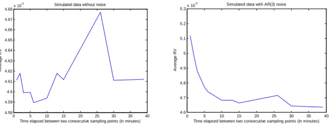
(26) We set the following values for the noise parameter: 0. = 0:5;. 1. = 0:5;. 1. = 0:5;. 2. = 0:2;. = 0:05:. 3. In order to make this simulation design less arbitrary, we will vary the autocovariances of "t;j . In fact, we have: !0. E "2t;j =. 0. 1+. 2 1. 2 2. +. +. 2 3. +. ! m;1. E ("t;j "t;j. 1). =. 0( 1. +. 1 2. ! m;2. E ("t;j "t;j. 2). =. 0( 2. +. 1 3). ! m;3. E ("t;j "t;j. 2). =. 0 3. ! m;h. E ("t;j "t;j. h). = 0 for all h. Because the link between ! 0 and ! 0 2 2:25. 0. = 0:05. 0. 0. in order to increase or decrease. = 1:2925 2 3). = 0:225. 0;. = 0:61. 0;. 0;. and. 4:. is one-to-one, we will directly vary ! 0 within the range:. 10. 8. ; 2:5. 10. 7. ; 2:25. 10. 6. ; 2:5. 10. 5. :. The value ! 0 = 2:5 10 7 has been used in Zhang and al. (2005) at …ve minute sampling frequency while ! 0 = 2:25 10 6 has served in Ait-Sahalia and al. (2005) at frequencies that range from one minute to thirty minutes. (L) We consider three IV estimators: the unbiased estimator 1;t (Equation (33)), the consistent estimator KtBN HLS with Bartlett kernel and the shrinkage estimator Kt$ with constant weight. After several trials, the bandwidth H = 0:4m2=3 seems to work well for KtBN HLS . In order to estimate the noise autocovariances, a …rst guess of the maximum lag L is needed. Although L = 3 b = 4 in the subsequent computations. A discussion on how to for the simulated noise, we set L formulate the …rst guess of L in practice is provided in the empirical section.. 6.2. Simulation Results. P (m ) First, we consider the volatility signature plots, that is, the curve of T1 Tt=1 RVt q plotted against m q = mq . Figure 2.1 describes one simulated sample without noise while Figure 2.2 describes a noisy version of the same data. It is seen that the volatility signature plots (at the top) are quite informative about the presence of the noise.. -5. 4.68. x 10. -5. Simulated data without noise 5.3. x 10. Simulated data with AR(3) noise. 4.67 5.2 4.66 5.1 Average RV. Average RV. 4.65 4.64 4.63 4.62 4.61. 5. 4.9. 4.8. 4.6 4.7 4.59 4.58. 0. 5 10 15 20 25 30 35 Time elapsed between two consecutive sampling points (in minutes). 4.6. 40. 0. 5 10 15 20 25 30 35 Time elapsed between two consecutive sampling points (in minutes). 40. Figure 2.1. Data with no noise. Figure 2.2. Data with MA(3) noise. Figure 2: Volatility Signature Plots.. 24.

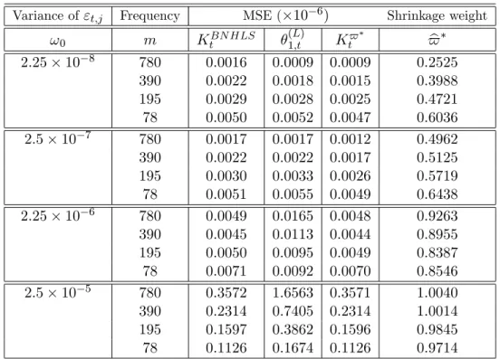
(27) c t of IVt , the empirical MSE of IV c t is given by: For any arbitrary estimator IV T 1X c c M SE(IV t ) = IV t T. IVt. 2. .. (52). t=1. c t . Table 2 displays the MSE of (L) , K BN HLS This MSE converges to the marginal variance of IV t 1;t and Kt$ for the e¢ cient price model with no leverage while Table 3 shows the results when leverage is included. Interestingly, we note that the introduction of leverage slightly reduces the variance in all the scenarios. Otherwise, the two tables display qualitatively similar results.. Variance of "t;j. !0 2:25. 10. 8. Frequency. MSE ( 10 6 ). m. KtBN HLS. 780 390 195 78 780 390 195 78 780 390 195 78 780 390 195 78. 0:0016 0:0022 0:0029 0:0050 0:0017 0:0022 0:0030 0:0051 0:0049 0:0045 0:0050 0:0071 0:3572 0:2314 0:1597 0:1126. (L) 1;t. 0:0009 0:0018 0:0028 0:0052 0:0017 0:0022 0:0033 0:0055 0:0165 0:0113 0:0095 0:0092 1:6563 0:7405 0:3862 0:1674. Shrinkage weight. Kt$. $ b. 0:0009 0:2525 0:0015 0:3988 0:0025 0:4721 0:0047 0:6036 7 2:5 10 0:0012 0:4962 0:0017 0:5125 0:0026 0:5719 0:0049 0:6438 6 2:25 10 0:0048 0:9263 0:0044 0:8955 0:0049 0:8387 0:0070 0:8546 5 2:5 10 0:3571 1:0040 0:2314 1:0014 0:1596 0:9845 0:1126 0:9714 Table 2: Evaluating the performance of the shrinkage estimators of IVt by Monte Carlo: Case with no Leverage E¤ect.. 25.

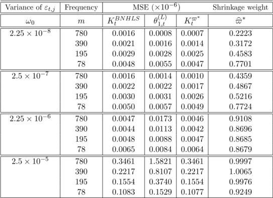
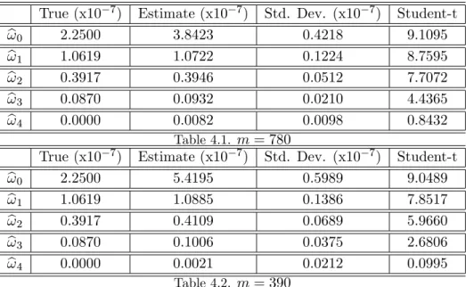
(28) Variance of "t;j. m. KtBN HLS. 780 390 195 78 780 390 195 78 780 390 195 78 780 390 195 78. 0:0016 0:0021 0:0029 0:0048 0:0016 0:0022 0:0030 0:0050 0:0047 0:0044 0:0048 0:0065 0:3461 0:2217 0:1554 0:1083. !0 2:25. 10. 8. MSE ( 10 6 ). Frequency. (L) 1;t. 0:0008 0:0016 0:0028 0:0055 0:0014 0:0022 0:0031 0:0057 0:0173 0:0113 0:0088 0:0084 1:5821 0:8107 0:3740 0:1529. Shrinkage weight. Kt$. $ b. 0:0007 0:2223 0:0014 0:3172 0:0025 0:4583 0:0047 0:7701 7 2:5 10 0:0010 0:4359 0:0017 0:4867 0:0026 0:5216 0:0049 0:7724 6 2:25 10 0:0046 0:9108 0:0042 0:8696 0:0047 0:8685 0:0064 0:8679 5 2:5 10 0:3461 0:9997 0:2217 1:0065 0:1554 0:9976 0:1077 0:9249 Table 3: Evaluating the performance of the shrinkage estimators of IVt by Monte Carlo: Case with Leverage E¤ect.. The e¢ cient return data has been contaminated with a Gaussian MA(3) microstructure noise driven by the same parameters regardless of the sampling frequency. Hence for a given ! 0 , the signal-to-noise ratio deteriorates as the sampling frequency increases. Likewise for a …xed sampling frequency, the signal-to-noise ratio deteriorates as ! 0 increases. It turns out that the optimal weight $ allocated to the consistent estimator heavily depends on the variance of the microstructure noise. In general, $ is increasing in ! 0 . In large ! 0 scenarios, the weight is close to one and decreases very slowly as m increases. By contrast, the weight is smaller in small ! 0 scenarios and increases quite fast as m decreases. Overall, the relative e¢ ciency gain of the shrinkage estimator over the consistent estimator is large when m is large and ! 0 is small. Note that compared to the consistent estimator KtBN HLS , the MSE of Kt$ is smaller by more than one half in the scenario (! 0 = 2:25 10 7 , m = 780) and by about one third for (! 0 = 2:25 10 7 , m = 390). (L) Not surprisingly, the inconsistent estimator 1;t performs better than the consistent estimator in small ! 0 scenarios (! 0 = 2:25. 10. 7 ).. In the large ! 0 scenarios (! 0 > 2:25. 10. 7 ), (L) 1;t. KtBN HLS. (L) 1;t. is not. preferred to at all the sampling frequencies while the best performance of is achieved at lower frequencies. This is consistent with the fact that the larger the noise variance ! 0 , the lower (L) the frequency that achives the optimal signal-to-noise ratio for 1;t . For a discussion on optimal sampling frequencies in the IID noise context, see for example Bandi and Russell (2006). Tables 4.1 and 4.2 show the estimation results for the correlogram of the noise in the scenarios (! 0 = 2:25 10 7 ; m = 780) and (! 0 = 2:25 10 7 ; m = 390) respectively. In these tables, the column labeled “True” contains the true values of the parameters. The estimates are computed using the Equation (44) while the standard deviations are computed from Equation (45) with ten lags. Firstly, we note that the estimator of ! 0 is biased upward and the bias decreases as the record frequency increases. In fact, the bias of ! b 0 is due to the presence of endogenous noise. Under the 26.

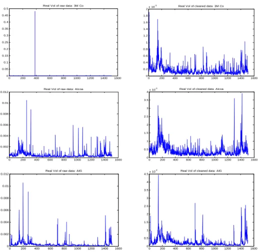
(29) assumption that. t;qk. is stationary, the unconditional bias of ! b 0 is given by:. E [b !0]. !0 =. 2 1. m. +. 1 (2 0. p. + 1) E m. t;qk. +. 0( 0. + 1) E. 2 t;qk. :. Hence while ! b 0 is biased for the variance of the exogenous noise, it does re‡ect the actual size of the total noise contaminating the price.. ! b0 ! b1 ! b2 ! b3 ! b4 ! b0 ! b1 ! b2 ! b3 ! b4. True (x10 2:2500 1:0619 0:3917 0:0870 0:0000. 7). True (x10 2:2500 1:0619 0:3917 0:0870 0:0000. 7). Estimate (x10 3:8423 1:0722 0:3946 0:0932 0:0082. 7). Std. Dev. (x10 0:4218 0:1224 0:0512 0:0210 0:0098 Table 4.1. m = 780 Estimate (x10 7 ) Std. Dev. (x10 5:4195 0:5989 1:0885 0:1386 0:4109 0:0689 0:1006 0:0375 0:0021 0:0212 Table 4.2. m = 390. 7). Student-t 9:1095 8:7595 7:7072 4:4365 0:8432. 7). Student-t 9:0489 7:8517 5:9660 2:6806 0:0995. Table 4: Estimated correlogram of the noise (Simulated Data).. The results suggest that the autocovariances estimators fb ! l g4l=1 are unbiased. The Student-t statistics displayed in the last column indicate that the null hypothesis ! 4 = 0 cannot be rejected at level 5%. This suggests that upon formulating a good initial guess of L, a standard t-test can be reliably used to assess the signi…cance of the noise autocovariances.. 7. Empirical Application. In the …rst subsection, we describe the data and discuss some methodological aspects of the empirical study. The results are presented in the second subsection.. 7.1. Data and Methodology. For this application, we use the data on twelve stocks listed in the Dow Jones Industrial8 . The prices are observed every one minute from January 1st , 2002 to December 31th , 2007 (1510 trading days). In a typical trading day, the market is open from 9:30 am to 4:00 pm, and this results in m = 390 observations per day. There are a few missing observations (less than 5 missing data per day) which we …lled in using the previous tick method. While our theoretical model assumes no jumps, the conclusions of many studies strongly suggest its presence in observed prices (see e.g Eraker (2004)). By assuming that the jumps are uncorrelated with both the e¢ cient price and the noise, we can perform our analysis by ignoring their presence. This does not a¤ect the estimators of the noise parameters, but the estimators Kt$ , KtBN HLS 27.

(30) (L). and 1;t are now designed the total quadratic variation which is equal to the IVt plus the jump contribution. To deal with outliers, we follow an intuition given in Barndor¤-Nielsen and al (2008b)9 by applying the following cleaning rule: N EW rt;j. OLD if r OLD rt;j t;j. =. OLD sign rt;j. rOLD. 50. ; rOLD otherwise. 50. OLD is the initial data and r OLD is the empirical median of r OLD across t and j. The where rt;j t;j N EW is treated as our initial observed return r N EW . This approach assumes that resulting rt;j rt;j t;j a jump must cannot be 50 times larger than the absolute median of the data. It has three main advantages. Firstly, it preserves the structure of dependence of the microstructure noise which is OLD contains substantial information about the of interest in our analysis. Secondly, the process rt;j normal range of the data, including the jumps. And thirdly, the median is known to be robust to outliers. Figure 3 show examples of the impact of this preprocessing on the data.. Real Vol of raw data: 3M Co. -3. 0.5. 2. 0.45. 1.8. 0.4. 1.6. 0.35. 1.4. 0.3. 1.2. 0.25. 1. 0.2. 0.8. 0.15. 0.6. 0.1. 0.4. 0.05 0. Real Vol of cleaned data: 3M Co. x 10. 0.2. 0. 200. 400. 600. 800. 1000. 1200. 1400. 0. 1600. 0. 200. 400. -3. Real Vol of raw data: Alcoa. 4. 0.012. 600. 800. 1000. 1200. 1400. 1600. 1200. 1400. 1600. 1200. 1400. 1600. Real Vol of cleaned data: Alcoa. x 10. 3.5 0.01. 3 0.008. 2.5 2. 0.006. 1.5 0.004. 1 0.002. 0.5 0. 0. 200. 400. 600. 800. 1000. 1200. 1400. 0. 1600. 0. 200. 400. -3. Real Vol of raw data: AIG 0.012. 4.5. 600. 800. 1000. Real Vol of cleaned data: AIG. x 10. 4 0.01 3.5 0.008. 3 2.5. 0.006 2 0.004. 1.5 1. 0.002 0.5 0. 0. 200. 400. 600. 800. 1000. 1200. 1400. 0. 1600. 0. 200. 400. 600. 800. 1000. OLD . Right: Realized volatility of r N EW . Figure 3: Preprocessing the data. Left: Realized volatility of rt;j t;j. We have suggested that L can be estimated by testing the signi…cance of f! m;h gL h=1 . However, the computation of these autocovariances requires the prior knowledge of L. We circumvent this. 28.

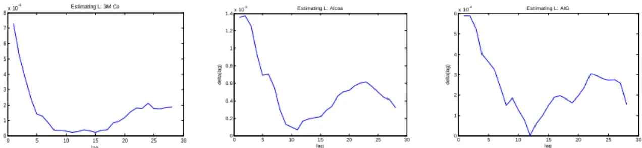
(31) vicious circle by using the following information criterion to obtain an initial guess of L: ( ) T X 2 1 (AC;m;l+1) H;T b = arg min L (l) = RV t ; H / m2=3 ; Kt T 0 l H 1. (53). t=1. (AC;m;l+1). where RV t. is de…ned as in (42) and:. KtH;T. =. T H 1 XX 1 + T. (Ac;m;1) RVt. h. 1 s;h. H. s=1 h=2. +. To see the intuition underlying the choice of this criterion, note that (AC;m;l+1). E [ (l)] = V ar KtH;T. RV t. h + E KtH;T. s; h. :. (l) satis…es: (AC;m;l+1). RV t. (AC;m;l+1). i2. is obtained by where the moments are taken unconditionally. On the one hand, RV t c t to l autocovariance terms and is thus unbiased for IVt when l L. truncating the expression of IV (AC;m;H) On the other hand, KtH;T is a smoothed version of RV t which is also unbiased for IVt due (AC;m;l+1). to L < H / m2=3 . Hence E KtH;T. RV t. is decreasing in l in the area l < L and equals (AC;m;l+1). is increasing in l, there is a trade-o¤ zero in the area l L. As the variance of KtH;T RV t between bias and variance that results in a L-shaped curve (l). See …gure 4.1. b given by (53) is used to compute the estimators of ! m;h ; h = 1; :::; L b + 1. If The initial guess L the signi…cance test indicates that the last two or three noise autocovariances are not signi…cantly b by di¤erent from zero, then the initial guess becomes our …nal estimator. Otherwise, we increment L +1 and repeat the process until the signi…cance test fails to reject the null for the last autocovariance.. 7.2. Empirical Results. We follow three basic steps in conducting this empirical study. In the …rst step, we estimate the b is used to compute the estimators of f! m;h gL , and memory parameter L. Next, the estimator L h=1 along with the relevant Student-t statistics. Finally, we compute the shrinkage estimator Kt$ . -4. 8. Estimating L: 3M Co. x 10. -3. 1.4. 7. 6. 1.2. 6. Estimating L: AIG. x 10. 5. 1 4. 5 4. 0.8. delta(lag). delta(lag). delta(lag). -4. Estimating L: Alcoa. x 10. 0.6. 3. 3 2 0.4. 2 1. 0.2. 0. 0. 0. 5. 10. 15 lag. 20. Figure 4.1: Plot of. 25. 30. 1. 0. 5. 10. 15 lag. 20. (l) against l. The minimum of. 29. 25. 30. 0. 0. 5. 10. 15 lag. 20. 25. (l) is used as the …rst guess of L.. 30.

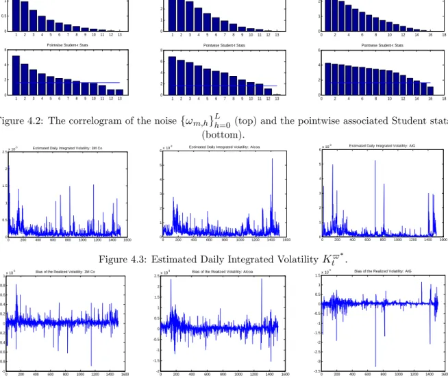
(32) -7. 1.5. -7. Correlogram of the noise: 3M Co. x 10. 4. -7. Correlogram of the noise: Alcoa. x 10. 3. 1. Correlogram of the noise: AIG. x 10. 3. 2. 2 0.5. 1. 1 0. 1. 2. 3. 4. 5. 6. 7. 8. 9. 10. 11. 12. 0. 13. 1. 2. 3. 4. Pointwise Student-t Stats. 5. 6. 7. 8. 9. 10. 11. 12. 0. 13. 0. 2. 4. 6. Pointwise Student-t Stats. 6. 8. 10. 12. 14. 16. 18. 14. 16. 18. 6. 6. 4. 8. Pointwise Student-t Stats. 4. 4 2. 2. 2 0. 1. 2. 3. 4. 5. 6. 7. 8. 9. 10. 11. 12. 0. 13. 1. 2. 3. 4. 5. 6. 7. 8. 9. 10. 11. 12. 0. 13. 0. 2. 4. 6. 8. 10. 12. L. Figure 4.2: The correlogram of the noise f! m;h gh=0 (top) and the pointwise associated Student stats (bottom). -3. 2.5. -3. Estimated Daily Integrated Volatility: 3M Co. x 10. 6. -3. Estimated Daily Integrated Volatility: Alcoa. x 10. 6. 5. 5. 4. 4. 3. 3. 2. 2. 1. 1. Estimated Daily Integrated Volatility: AIG. x 10. 2. 1.5. 1. 0.5. 0. 0. 200. 400. 600. 800. 1000. 1200. 1400. 0. 1600. 0. 200. 400. 600. 800. 1000. 1200. 1400. 1600. 0. 0. 200. 400. 600. 800. 1000. 1200. 1400. 1600. Figure 4.3: Estimated Daily Integrated Volatility Kt$ . -3. 1. -3. Bias of the Realized Volatility: 3M Co. x 10. 2.5. 0.8. -3. Bias of the Realized Volatility: Alcoa. x 10. 1.5 1. 2. 0.6. Bias of the Realized Volatility: AIG. x 10. 0.5. 1.5. 0. 0.4. 1. -0.5. 0.2. 0.5. -1. 0. 0. -1.5. -0.2. -0.5. -0.4. -2.5. -1.5. -0.8 -1. -2. -1. -0.6. 0. 200. 400. 600. 800. 1000. 1200. 1400. 1600. -2. -3 0. 200. 400. 600. 800. 1000. 1200. 1400. 1600. -3.5. 0. 200. 400. 600. 800. 1000. 1200. 1400. 1600. Figure 4.4: Estimated Bias of the Realized Volatility RV (m) . Figure 4: Estimation Results for 3M Co, Alcoa and AIG.. Figure 4.1. shows the plots of (l) against L while Figure 4.2 shows the estimated noise autocovariances along with the signi…cance tests for the assets 3M Co, Alcoa and AIG. This …gures suggets that the initial guess of L slightly overestimates the value predicted by the signi…cance test. The estimated values of L for the other assets are displayed in Table 5. For all the stocks considered, our results suggest that the noise is L-dependent with values of L lying between 5 minutes (American Express) and 14 minutes (AIG and General Electric). The …nding that the noise is autocorrelated is not new in the literature10 . However, we contribute to the discussion by showing that there is a vicious circle raised by the determination of L and we propose a way to solve this. Figure 4.3 and Figure 4.4 show respectively the time series of Kt$ and the resulting estimated bias of the RV ebt = RV (m) Kt$ . This alternative formula is preferred for the bias because it (m) has less variance compared to the natural method of moment estimator bbt given in (41). To compute the realized kernels, we set H = 30 for the bandwidth except for the American Express index (AXP) which necessitates H = 10. These bandwidth values appear to produce better results than (390)2=3 ' 53. Figure 4.4 suggests that the sign of ebt is not constant through time. It turns 30.

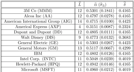
(33) out that when the correlogram is positive as we found for 3M Co, Alcoa and AIG, a negative bias can only be due to a negative correlation between the noise and the latent return. This suggests that either 0 or 1 is negative. b b (b b ) 3M Co (MMM) 0:5301 (0:1841) 0:4165 Alcoa Inc (AA) 0:4797 (0:0278) 0:4165 American International Group (AIG) 0:4715 (0:0100) 0:4423 Americal Express (AXP) 0:3151 (0:0087) 0:2324 Dupont and Dupont (DD) 0:4805 (0:0111) 0:4165 Walt Disney (DIS) 0:4773 (0:0132) 0:3683 General Electric (GE) 0:5303 (0:0267) 0:4423 General Motors (GM) 0:5117 (0:0667) 0:4299 IBM 0:4802 (0:0126) 0:4165 Intel Corp. (INTC) 0:5048 (0:0239) 0:4019 Hewlett-Packard (HPQ) 0:4942 (0:0146) 0:4165 Microsoft (MSFT) 0:4960 (0:0212) 0:4019 Table 5: Estimates of L, and for twelve stocks listed in the DJI. b b is the estimated standard deviation of b b L 12 12 14 4 12 9 14 13 12 11 12 11. Table 5 shows the estimates b and b. It is seen that b < b < 2=3 for all the assets. In our framework, the fact that the inequality b < b is satis…ed indicates that the noise process has …nite variance, while b < 2=3 indicates that the estimator of Barndor¤-Nielsen and al. (2008a) delivers its best performance at the highest available frequency. Finally, note that the value of b can still be used as a measure of persistence of the microstructure noise even if assumption E4 is not satis…ed.. 8. Conclusion. This paper proposes a ‡exible semi-parametric model for the market microstructure noise. We specify the microstructure noise as the sum of two terms. The …rst term is correlated with the latent return and the second term is exogenous. The exogenous noise is modeled as an L-dependent process, where L is allowed to increase with the frequency at which the prices are recorded. In light of this model, we study the properties of common realized measures that aim to estimate the integrated volatility. We propose a new shrinkage realized kernels which is an optimal linear combination of the consistent realized kernels of Barndor¤-Nielsen and al (2008a) and an unbiased estimator constructed for this purpose. It is shown theoretically that the shrinkage estimator has lower variance than the consistent estimator in small samples while both estimators are asymptotically equivalent in large samples. The Monte Carlo simulations show that the relative e¢ ciency gain of the shrinkage realized kernels over the standard realized kernel is substantial in situations where the variance of the microstructure noise is small. When the variance of the noise is large, the inconsistent estimator is markedly dominated. Finally, we propose a framework to assess the true values of the noise parameters via the observed returns. Unfortunately, the endogeneity parameters are not identi…ed. Our empirical …ndings about the noise con…rm the conclusions of Hansen and Lunde (2006): there is strong evidence that the 31.

(34) noise is autocorrelated and correlated with the latent returns. If our Assumption E3-E3 are true, p then the rate at which L increases with the sampling frequency is in general slower than m. Acknowledgement 6 We wish to thank Torben Andersen, Valentina Corradi, Prosper Dovonon, Rene Garcia, Silvia Goncalves, Ilze Kalnina, Nour Meddahi, the Associate Editor and two anonymous referee for helpful comments. An earlier draft of this paper has circulated under the title “Assessing the Nature of Pricing Ine¢ ciencies via Realized Measures”.. 32.