Choice of contract maturity with applications to international and mortgage lending

AVIS

Ce document a été numérisé par la Division de la gestion des documents et

des archives de l’Université de Montréal.

L’auteur a autorisé l’Université de Montréal à reproduire et diffuser, en totalité

ou en partie, par quelque moyen que ce soit et sur quelque support que ce

soit, et exclusivement à des fins non lucratives d’enseignement et de

recherche, des copies de ce mémoire ou de cette thèse.

L’auteur et les coauteurs le cas échéant conservent la propriété du droit

d’auteur et des droits moraux qui protègent ce document. Ni la thèse ou le

mémoire, ni des extraits substantiels de ce document, ne doivent être

imprimés ou autrement reproduits sans l’autorisation de l’auteur.

Afin de se conformer à la Loi canadienne sur la protection des

renseignements personnels, quelques formulaires secondaires, coordonnées

ou signatures intégrées au texte ont pu être enlevés de ce document. Bien

que cela ait pu affecter la pagination, il n’y a aucun contenu manquant.

NOTICE

This document was digitized by the Records Management & Archives

Division of Université de Montréal.

The author of this thesis or dissertation has granted a nonexclusive license

allowing Université de Montréal to reproduce and publish the document, in

part or in whole, and in any format, solely for noncommercial educational and

research purposes.

The author and co-authors if applicable retain copyright ownership and moral

rights in this document. Neither the whole thesis or dissertation, nor

substantial extracts from it, may be printed or otherwise reproduced without

the author’s permission.

In compliance with the Canadian Privacy Act some supporting forms, contact

information or signatures may have been removed from the document. While

this may affect the document page count, it does not represent any loss of

content from the document.

Choice of Contract Maturity with Applications to

International and Mortgage Lending

par

Albert Le Grand Touna Marna

Département de sciences économiques

Faculté des arts et sciences

Thèse présentée

à

la Faculté des études supérieures

en vue de l'obtention du grade de Philosophire Doctor (Ph.D.)

en sciences économiques

Décembre, 2008

@Albert Le Grand Touna Marna, 2008.

Faculté des études supérieures

Cette thèse intitulée :

Choice of Contract Maturity with Applications to

International and Mortgage Lending

présentée par :

Albert Le Grand Touna Mama

a été évaluée par un jury composé des personnes suivantes :

Alessandro Riboni, président-rapporteur

Rui Castro,

directeur de recherche

Michel Poitevin,

co-directeur de recherche

Bari§ Kaymak,

membre du jury

Christian Sigouin,

examinateur externe

, représentant du doyen de la FAS

Cette thèse contribue à la littérature sur la durée des contrats en identifiant les bénéfices et les coûts de l'engagement de long terme dans le cas des contrats de dette internationale, et dans le cas des contrats d'emprunt hypothécaire; notamment du point de vue de l'agent. Plus précisément, je caractérise et compare deux structures alternatives de contrats de dette qui diffèrent uniquement par l'ajustement qu'elles prévoient face à un changement exogène du taux d'intérêt futur. D'une part, un contrat de long terme qui ne prévoit aucun ajustement des remboursements au taux d'intérêt réalisé, et de ce fait constitue un instrument sans risque pour l'emprunteur. D'autre part, un contrat de court terme qui prévoit un ajustement complet des remboursements, et de ce fait constitue un instrument risqué pour l'emprunteur. Intuitivement, le choix de s'engager à long terme est semblable au choix entre un actif à rendement sans risque et un actif à rendement risqué. Les facteurs importants qui déterminent la durée du contrat sont le degré d'aversion pour le risque et le profil de revenu de l'emprunteur .

Dans le chapitre 1, mon modèle de choix de la durée des contrats permet d'expliquer le recours aux contrats d'hypothèque à taux flexible par des agents averses au risque. Ma contribution, à la littérature sur le choix de contrats d'hypothèque, est de montrer que les contrats d'hypothèque à taux variable permettent aux agents de s'auto assurer contre le risque de taux, en ajustant leurs paiements en conséquence. Sous certaines conditions, renoncer à l'assurance d'un contrat

d'hypo-thèque à taux fixe est optimal. Dans le chapitre 2, j'estime une forme réduite du modèle de choix de contrats d'hypothèque, basée sur les résultats du chapitre 1. Je compare mes estimations aux résultats présents dans la littérature empirique. La contribution de ce chapitre est de mettre à profit une nouvelle base de données pour étudier le choix de contrats d'hypothèque. Dans le chapitre 3, mon modèle de choix de la durée des contrats permet d'expliquer le recours excessif, dans les années 1990, à la dette extérieure de court terme par les pays émergents. Ma contribution, à la littérature sur les mouvements de capitaux internationaux, est de montrer que la dette de long terme et la dette de court terme sont des substituts imparfaits. Toute politique visant la réduction de l'endettement à court terme devrait proposer des instruments alternatifs.

Mots-clés: Hypothèque à taux fixe, Hypothèque à taux variable, Crise asiatique, Dette extérieure

Abstract

This dissertation contributes to the literature of contract length by identifying benefits and costs of long-term commitment in the case of both foreign debt contracts, and mortgage loan contracts; in particular from the borrower point of view. More precisely, 1 characterize and compare two alternatives structures of debt contracts which differ only by the extent to which they accommodate for an exogenous shock on the future interest-rate. On one hand, long-term contracts do not adjust to the realized interest-rate, so that they are risk-free for the borrower. Short-term contracts on the other hand, adjust the repayments to the realized rate of interest. Therefore, they are risky for the borrower. Intuitively, the choice of long-term commit ment is similar to the choice between a risky asset and a risk-free asset. The key factors that govern this choice are both the degree of risk aversion, and the income profile of the borrower.

ln the first chapter, my model of maturity choice helps explain why risk-averse borrowers choose adjustable-rate mortgage contracts. My contribution, specifically to the literature on mortgage choice, is to prove that adjustable-rate mortgage loans allow for self-insurance against the interest-rate risk, by adjusting repayments consequently. Under sorne conditions, it becomes optimal to renounce to the insurance attached to fixed-rate mortgage loans. In the second chapter, 1 run an estimation of a reduce-form equation, based on Chapter l's findings. Then, 1 compare the estimates with the corresponding empirical literature. The novelty in this chapter cornes from using a new

database on mortgage indebtedness. In the third chapter, my model of maturity choice helps ex-plain the surge in short-term foreign borrowing by Emerging countries prior to the Asian crisis. My contribution, specifically to the literature on international capital flows, is to prove that long-term and short-term debt instruments are imperfect substitutes. Henee, any policy aiming at discoura-ging short-term indebtedness should propose alternatives instruments.

Key words: Fixed-rate mortgage, Adjustable-rate mortgage, Asian crisis, Maturity mismatch, Precautionary saving, Flexibility, Self-insuranee, Contract length.

Résumé

Abstract iii

Liste des figures viii

Liste des tableaux

Dédicace

Remerciements

Introduction

1 Households' choice between fixed- and adjustable-rate mortgages : On the value of flexibility in contracting

1.1 Introduction . . . . 1.2 Summary of previous research . 1.3 The model. . . . .

1.4 Mortgage contracts

1.4.1 Fixed-rate mortgage contracts . 1.4.2 Adjustable-rate mortgage contracts . 1.5 Determinants of the mortgage choice . . . .

1.5.1 Borrower's attitude towards interest-rate risk 1.5.2 Borrower's allocation of risk over time . . . .

v ix x xi 1 6 7 8 11 13 13 15 17 19 23

1.6 Mortgage choice with constant relative risk aversion 1.6.1 The effect of uncertainty . . . . 1.6.2 The effect of consumption smoothing . 1. 7 Conclusion and Empirical implications . . . .

2 Households' choice between ftxed- and adjustable-rate mortgages : An Empirical 26 27 32 32 Analysis 34 2.1 Introduction. 35 2.2 Literature review 37 2.3 Data

2.3.1 Background on U.S. mortgage market 2.3.2 Description and selection

2.4 Preliminary analysis . . 2.5 Empirical methodology . 2.6 Empirical results 2.7 Conclusion.... 39 39

41

50 55 56

60

3 On the Maturity Structure of Foreign Debt Contracts in Emerging Countries 62

3.1 Introduction... 63

3.2 A simple contracting game . 3.2.1 The setup . . . . 3.2.2 Contracting options 3.3 Preliminary analysis . . . .

3.3.1 Rewriting the long-term problem 3.3.2 Unfeasibility of contingent contracts

3.3.3 Country's attitude toward interest rate volatility 3.4 Debt maturity choice and interest rate volatility . 3.5 Debt maturity choice and economic growth

3.5.1 The effect of growth : intuition 3.5.2 The effect of growth : analytic . 3.6 Empirical analysis . . . .

67

67

68

71 71 72 72

74

79 79 79 83

3.7 Conclusions and policy implications. . . .. 87 Conclusion 89 Bibliographie 90 0.1 Introduction générale.

0.2

Chapter one .

0.3

Chapter two .

0.4

Chapter three Annexes .1 Chapter one .

.1.1 Sketch of the mort gage problem .

. 1.2 A value of information perspective of the ARM problem .1.3 Curvature of the indifference curve

.1.4

Sorne calculations . .1.5 Proof . . . . .1.6 Mortgage choice .2 Chapter two . . . .

.3

.2.1

.2.2

Data definitions and sources . Benchmark interest-rate . . .

.2.3 Estimating Risk Tolerance from the 1996 PSID by Ming-Ching Luoh and Frank Stafford

Chapter three . . . .

.3.1

V's curvature

.3.2

Proof

....

.3.3

Approximation of Cl in the short-term agreement.

.3.4

Partial derivative of WST _{and W}LT _{wrt to w}

.3.5

Data definitions and sources . . . .

92 92 95

97

101

102

102

103

104

105

107

108

109

109

111

112

113

113

113

114

118

118

Table des figures

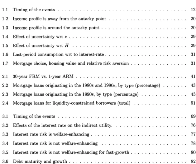
1.1 Timing of the events . . . . 1.2 Income profile is away from the autarky point 1.3 Income profile is around the autarky point 1.4 Effect of uncertainty wrt 1/ .

1. 5 Effect of uncertainty wrt H

1.6 Last-period consumption wrt to interest-rate .

1.7 Mortgage choice, housing value and relative risk aversion.

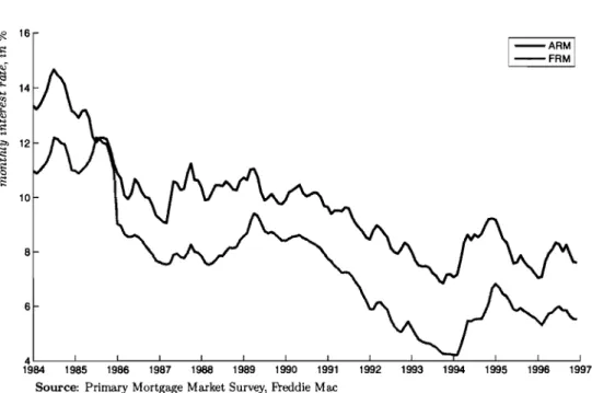
2.1 30-year FRM vs. 1-year ARM . . . .

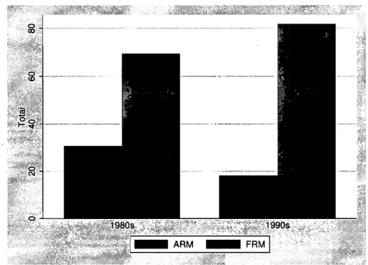
2.2 Mortgage loans originating in the 1980s and 1990s, by type (percentage) 2.3 Mortgage loans originating in the 1990s, by type (percentage)

2.4 Mortgage loans for liquidity-constrained borrowers (total)

3.1 Timing of the events . . . . 3.2 Effects of the interest rate on the indirect utility. 3.3 Interest rate risk is welfare-enhancing. . . 3.4 Interest rate risk is not welfare-enhancing

3.5 Interest rate risk is not welfare-enhancing for fast-growth . 3.6 Debt maturity and growth . . . .

12 20 20 29 29 31 31 41 43 43 51 69 76 77 78 80 82

Liste des tableaux

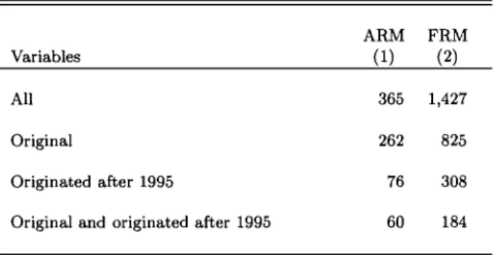
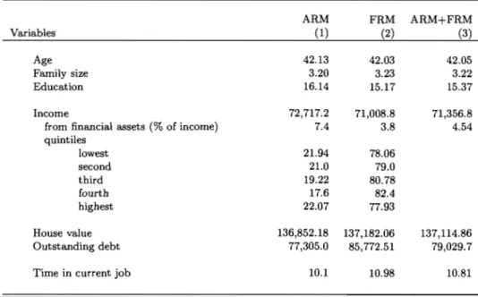
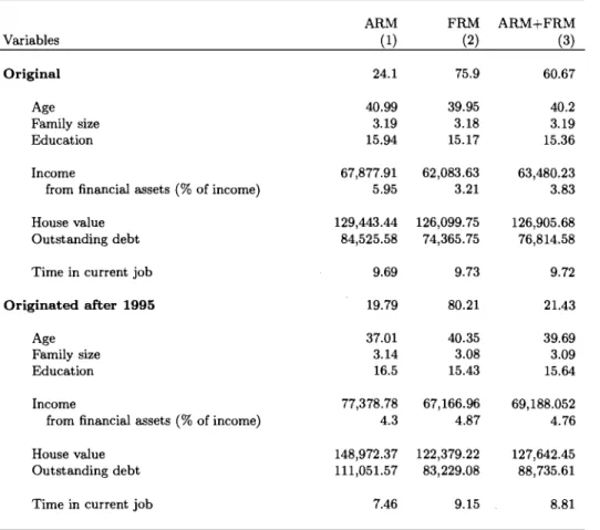
2.1 Mortgage selection for various sub-samples (total) . . . . 2.2 Mortgage selection and sociodemographic characteristics (proportion) 2.3 Mortgage selection and sociodemographic characteristics, all (average) 2.4 Mortgage selection and sociodemographic characteristics, by sub-samples 2.5 Mortgage selection by occupation (proportion) . . . . 2.6 Mortgage selection and sociodemographic characteristics, by liquidity status 2.7 Mortgage selection and sociodemographic characteristics, by mobility status

2.8 PROBIT ESTIMATES OF THE MORTGAGE CHorCE . . . .

3.1 Short-term external debt, growth and market volatility",b . . . . 2 Mortgage choice, housing value (H) and relative risk aversion (v)

44

45

47

48

49

52

54

58

86

109

à mes parents

Remercien1ents

Je remercie mes directeurs de thèse Rui Castro et Michel Poitevin pour leur encadrement et pour leur disponibilité. Votre patience m'a grandement aidé à construire mon esprit de chercheur; et votre rigueur à acquérir la maturité de la remise en question.

Je remercie maman, papa, Christiane, Dominique et Ange-Emmanuel pour leur confiance in-défectible. Votre amour, votre présence et vos encouragements ont été déterminants pour que ce projet se réalise.

Cette thèse n'aurait pas vue le jour sans l'environnement social dans lequel j'ai vécu depuis mon départ du Cameroun. Je tiens à remercier la famille Poulon, la famille Lafaye, la famille du Mas des Bourboux, la famille Salabanzi, Henri-Michel Nsom Mengo, Lionel Namtchueng, Diomède Noukeu, Ngomba Armelle, Loyal Chow, Yolande Tchitchi, Maude Ruest-Archambault, Dahlia Attia, Dorothée Le Garrec, David Djoumbissie, Selma Chaker, Eric Bahel, Marne Astou Diouf, Marna Keita, Isabelle Akaffou, Markus Herrmann, Bertille Antoine, Aurélie Deffo, Carlos de Resende, Clarence Tsimpo, Sherine Attia, Pascal Martinolli, Jacques Ewoudou, Fulbert Tchana Tchana et Anne-Constance Lenthé. Merci pour l'équilibre que vous m'avez apporté.

Je remercie tout le personnel enseignant et administratif du département de sciences économiques de l'Université de Montréal pour leur support intellectuel et logistique tout au long de ce projet. Je remercie en particulier Alessandro Riboni, Walter Bossert, Gérard Gaudet, André Martens, Suzanne

Larouche-Sidoti, Lyne Racine et Abdoulaye Diaw.

Je suis reconnaissant envers le département de sciences économiques de l'Université de Montréal,

1e ClREQ, la Banque du Canada, le Fonds Monétaire Internationa1, le Ministère de l'enseignement

supérieur du Cameroun pour leur soutien financier direct ou indirect tout au long de mes années de

doctorat.

Je rends grâce au Seigneur pour m'avoir accordé 1a santé et la persévérance pour mener ce projet

Introduction

Dans plusieurs situations réelles pour lesquelles une analyse de type principal-agent semble

adaptée, la durée est un paramètre dé d'un contrat entre parties. L'intérêt pour la durée des

contrats découle du tait qu'elle puisse être différente de la durée de la relation entre les parties.

Sur le marché du travail, par exemple, un employeur et un employé d'une industrie saisonnière

signent généralement un contrat à durée déterminée mais qu'ils renouvellent chaque saison. Il en va de même pour certains contrats de dette sur les marchés des capitaux. Afin de rembourser un

emprunt lié à l'achat d'une maison, une banque et un ménage peuvent signer plusieurs contrats d'emprunt, successifs, de durée unitaire inférieure à la durée de l'amortissement. D'un point de vue aussi bien normatif que positif, il est important de comprendre dans quelle mesure la durée d'un

contrat devrait dépendre des facteurs environnants.

En l'absence de toutes frictions dans l'économie, des parties entrant dans une relation de plusieurs

périodes devraient signer un contrat de long terme couvrant toute la durée de leur relation, et

prenant en compte toutes les contingences possibles liées à la relation. Il en découle que, expliquer la durée des contrats reviendrait à expliquer les bénéfices et les coûts associés à l'engagement de long terme. En pratique, par exemple, l'absence de contrats complets serait due au coût prohibitif de la

spécification et de l'application de toutes les contingences possibles (Williamson (1985)). Les études

est la durée optimale d'un contrat? Et, sous quelles conditions une succession de contrats de court terme est aussi efficiente qu'un contrat de long terme?

Premièrement, les recherches sur la durée optimale d'un contrat concluent qu'elle dépend du degré d'incertitude qui affecte les parties, indépendamment du fait que cette incertitude soit exogène ou non, idiosyncrasique ou non. Parmi les pionniers de cette littérature, Gray (1978) a montré que la durée optimale d'un contrat est négativement reliée au niveau d'incertitude. Dans le modèle de Gray, la durée optimale est telle qu'elle minimise le coût total moyen de contracter (coût de transaction) sur la période du contrat. Un contrat de long terme possède l'avantage d'amortir sur une période plus longue les coûts fixes liés à la négociation du contrat. Tandis qu'un contrat de court terme, réduit les coûts liés à l'incertitude. En effet, Gray suppose que le degré d'incertitude augmente dans le temps. D'autres études ont nuancé la conclusion de Gray (1978). Harris et Holmstr6m (1987) ont montré que si les coûts de transactions augmentent avec le niveau d'incertitude, alors il est possible que la durée optimale du contrat augmente aussi avec le niveau d'incertitude. Dans le modèle de Harris et Holmstr6m, le coût est lié à l'acquisition de l'information sur l'unique variable d'état du système (et du contrat). Le choix d'acquérir de l'information s'apparente à réduire la durée du contrat. Aussi, lorsque le niveau d'incertitude augmente l'information se détériore, mais plus rapidement que l'augmentation du niveau d'incertitude. Au delà d'un certain seuil les pertes liées à la non-acquisition de l'information deviennent supérieures au coût de son acquisition. Enfin, Dye (1985) a montré que la durée optimale d'un contrat varie dans le temps, et sous certaines conditions est indépendante du niveau d'incertitude.

Deuxièmement, une succession de contrats de court terme est aussi efficiente qu'un contrat de long terme lorsque trois conditions sont réunies. Selon la première condition, l'agent n'a pas accès aux marchés des capitaux tandis que le principal y a un accès illimité. Selon la deuxième

condition, aux dates de renégociation, l'information nécessaire pour identifier toutes contingences pertinentes est connaissance commune. Et enfin selon la troisième condition, le principal et l'agent maximisent des objectifs conflictuels, de sorte que la frontière de Pareto soit décroissante. Sous ces conditions, Malcomson et Spinnewyn (1988) et Rey et Salanié (1990) ont montré que le lissage optimal de la consommation peut être atteint indépendamment du type de contrats. Fudenberg, Holmstrom et Milgrom (1990) arrivent au même résultat en supposant que l'agent possède un accès illimité aux capitaux au même taux d'intérêt que le principal, pourvu que les parties possèdent la même information aux dates de renégociation. Pour éliminer l'information asymétrique découlant de l'accès de l'agent aux marchés des capitaux, il suffit par exemple que la fonction d'utilité de ce dernier exclue les effets de richesse.

Cette thèse contribue à la littérature sur la durée des contrats en identifiant les bénéfices et les coûts de l'engagement de long terme dans le cas des contrats de dette internationale, et dans le cas des contrats d'emprunt hypothécaire; notamment du point de vue de l'agent. Plus précisément, je caractérise et compare deux structures alternatives de contrats de dette qui diffèrent uniquement par l'ajustement qu'elles prévoient face à un changement exogène du taux d'intérêt futur. D'une part, un contrat de long terme qui ne prévoit aucun ajustement des remboursements au taux d'intérêt réalisé, et de ce fait constitue un instrument sans risque pour l'agent.l D'autre part, un contrat de court terme qui prévoit un ajustement complet des remboursements, et de ce fait constitue un instrument risqué pour l'agent. Implicitement, la durée des contrats est supposée exogène, et négativement corrélée au niveau d'incertitude compris dans le contrat. En l'absence d'incertitude dans l'économie, il est équivalent de signer un contrat de long terme ou une succession de contrats de court terme.2

1 Je suppose que le principal absorbe tout le risque. 2Lorsque la variance du taux d'intérêt futur est nulle.

Dans le cas plus général où l'incertitude est présente, le choix de s'engager ou non à long terme est semblable au choix entre un actif à rendement sans risque et un actif à rendement risqué. Ainsi, les facteurs importants qui déterminent le choix d'un contrat sont le degré d'aversion pour le risque et le profil de revenu de l'agent. Je montre, par exemple, que les bénéfices de l'engagement à long terme augmentent avec le degré d'aversion au risque. Intuitivement, plus un agent est averse au risque plus il bénéficie de l'assurance du contrat de long terme, toutes choses égales par ailleurs. Tandis que les coûts de l'engagement à long terme augmentent avec le niveau de revenus accumulés avant l'occurrence du choc sur le taux d'intérêt. Intuitivement, plus un agent est riche plus il est capable de s'auto assurer, toutes choses égales par ailleurs.

Dans le chapitre 1, mon modèle de choix de la durée des contrats permet d'expliquer le recours aux contrats d'hypothèque à taux flexible par des agents averses au risque. Ma contribution, à la littérature sur le choix de contrats d'hypothèque, est de montrer que les contrats d'hypothèque à taux variable permettent aux agents de s'auto assurer contre le risque de taux, en ajustant leurs paiements en conséquence. Sous certaines conditions, renoncer à l'assurance d'un contrat d'hypothèque à taux fixe est optimal. Dans le chapitre 2, j'estime une forme réduite du modèle de choix de contrats d'hypothèque, basée sur les résultats du chapitre 1. Je compare mes estimations aux résultats présents dans la littérature empirique. La contribution de ce chapitre est de mettre à profit une nouvelle base de données pour étudier le choix de contrats d'hypothèque. Mes estimations permettent de conclure que le degré d'aversion au risque et le niveau de richesse du ménage sont des facteurs importants du choix de contrats d'hypothèque. Dans le chapitre 3, mon modèle de choix de la durée des contrats permet d'expliquer le recours excessif, dans les années 1990, à la dette extérieure de court terme par les pays émergents. Ma contribution, à la littérature sur les mouvements de capitaux internationaux, est de montrer que la dette de long terme et la dette de

court terme sont des substituts imparfaits. Toute politique visant la réduction de l'endettement à

Chapitre 1

Housel10lds' choice between fixed- and

adjustable-rate n10rtgages : On the value

of flexibility in contracting

1.1 Introduction

Mortgage choice is an important decision that many households make at least once in their lifetime. Because of the many dimensions in which mortgage loans can differ (caps, margins, pre-payment, points, refinancing charges, ... ), such a choice is very complex one. At the very least howe-ver, practitioners and economists classify mort gages between fixed-rate (FRM) and adjustable-rate (ARM), that is according to their adjustability to interest-rate changes. Under an FRM contract, the coupon rate is fixed once-and-for-all at the time the contract is signed. Under an ARM on the other hand, the coupon rate is adjusted to a given index at pre-specified intervals. As a result, FRM contracts insulate borrowers against interest-rate risk, so that uncertainty is borne entirely by the lender. On the contrary, ARM contracts reflect the risk of rising interest-rates to borrowers. We are concerned with how households' idiosyncrasies influence their mort gage choice along this classification. Beyond the intuitive role of risk aversion as favoring FRM contracts (see for instance Capozza and Gau (1983)), the theoreticalliterature has yet to explain how a risk-averse borrower can benefit from interest-rate risk in the first place.

ln this paper, we investigate the idea that the flexibility that cornes with an ARM contract should promote such risk taking. Indeed, peculiar to the mortgage choice is the fact that interest-rate uncertainty gets resolved before the mortgage contract cornes to an end. Thus, the borrower is able to self-insure by spreading this risk over the subsequent periods that follow resolution. It can be accomplished by setting the remaining payments so as to reduce the overall exposure to risk; something possible under an ARM contract as payments are contingent to interest-rate realizations. This in turn should incite risk-averse individuals to bear risk, provided that they are better-off than under an FRM contract.1

lIn this respect, the mort gage choice is an illustration that the optimal attitude toward risk and the way this risk will be allocated cannot be dissociated (see Gollier (2002)).

We opt for a three-period model, where a risk averse household must finance the purchase of a house from a deterministic income stream. The future interest rate is uncertain and the only means to transfer resources over time are : an adjustable-rate mortgage or a fixed-rate mortgage. The model predicts, among other things, that : more risk averse households are more likely to select FRM loans over ARM loans because they tend to shy away from fluctuating consumption paths as those implied by the repayment schedules of ARM loans. Moreover, for households with similar wealth, those with a faster income growth are more likely to choose FRM loans because a higher share of their discounted lifetime income is subject to uncertainty. Finally, households which are sufficiently rich prior to the interest-rate adjustment, are more likely to select adjustable-rate loans over fixed-rate loans. In fact, they enjoy similar advantages as investing in a risky asset while being able to self-insure against interest-rates increases.

The rest of the paper is organized as foHows. Section 2 presents the environment. Section 3 displays the mechanisms between the mortgage choice. Section 4 presents the self-insurance effect. In section 5, we consider the case of CRRA utility function. In section 6, we conduct an empirical investigation of the model implications. Conclusions are presented in section 7.

1.2 Summary of previous research

Few papers theoretically discuss the choice between adjustable-rate and fixed-rate mortgages, let alone provide a rationale for choosing ARM loans. Capone and Cunningham (1992) sketch the importance of risk aversion and holding periods. However, their analysis ignores self-insurance as they find no rationale for risk-averse borrowers to hold ARMs, when FRMs with the same holding period are available. Baesel and Biger (1980) and Statman (1982) focus on inflation and labor income. AH these papers approach the demand for mort gage in the specific case where a borrower

maximizes the expected utility of its lifetime wealth at retirement, with no intermediary consumption

on which to spread interest-rate risk.2 However, it shotild only be under restrictive circumstances that the repayment schedule (and de facto mortgage demand) is unrelated to a borrower's lifetime consumption profile.3 _{The reason is that the typical household portfolio is quite undiversified. A} mortgage loan is usually its major liability (see Guiso et al. (2001)) which, in addition, is carried over a long portion of its lifetime.4 _{A notable exception to this special case, however, has been} Campbell and Cocco (2003).

Campbell and Cocco numerically solve a life-cycle model and assume a constant relative risk aversion utility (CRRA). They find that households with smaller houses relative to income, more stable in come and lower risk aversion should find ARMs most attractive. AU this is consistent with our theoretical analysis based on a CRRA utility function (section 6). But Campbell and Cocco (2003) make no mention of the underlying assumptions, as we do in this paper. We are not aware of any previous work that treats early resolution of uncertainty in the mortgage choice.

Empirical studies, on the other hand, have highlighted the central role of borrowers' risk aversion in the mortgage choice decision. Capone and Cunningham (1992) find that, for any given holding period, borrowers who choose ARM contracts have lower degrees of risk aversion. In Sa-Aadu and Sirmans (1995), this role shows up through a life-cycle effect, as younger households appear more sensitive to interest-rate changes than older borrowers.5 Using Canadian data, Breslaw, Irvine and

2Gollier (2002) provided the theoretical foundation of allocating risk on consumption over several periods after uncertainty is resolved.

3Evidence of correlations between mortgage-related features and lifetime consumption profiles can be found in Englehardt (1996). Using data drawn from the PSID, he find that down payment constraints affect consumption profiles by forcing first-time home buyers to reduce consumption when young in order to access to homeownership later on.

4Canada is no exception as mortgages are the single most important debt; accounting for 75% of the overall value (see Statistics Canada (2005)). Guiso et al. (2001) also found that a house is usually the major asset in the typical household portfolio. Ironically, and contrary to the literature on the demand for mortgage, the literature on the demand for housing has long operated within the !ife-cycle framework (see for example Dusansky and Wilson (1993)).

5 Liquidit Y constraints is a factor as weil. Since old households are less likely to face binding constraints, they can afford to take more risk than young households.

Rahman (1996) found that borrowers with family responsibilities also display relatively more aver-sion to interest-rate risk. Campbell and Cocco (2003) examine the mortgage choice in a dynamic stochastic equilibrium model. They demonstrate that risk aversion is important in generating pat-terns that are consistent with V.S. data.

1.3 The model

There are two individuals, a borrower and a lender. They live for three periods. The borrower's

consumption in period t is denoted by Ct

>

0, for all

t.

Preferences are time-separable, and

ma-mentary utility is given by the function u which is continuous, thrice differentiable with u' > 0 and

u"

< O. We impose the Inada condition lim u'

(C) =

+00.

For each period, the borrower earns an

C--+O

income

Yt >

0 units of the consumption good. This income stream is nonstochastic. The borrower

enters the first period having signed a mort gage contract for the purchase of a house worth H units

of consumption.6 The house is to be paid in the remainder of the agent's life. Let Dt denote period

t's repayment.

The lender is risk neutral, it only cares about the total discounted mortgage payments and not

about their timing. It can borrow or save unlimited amounts at the market (gross) rate of interest

Rt, between t and t

+

1; RI is fuced, but we assume that R2 is stochastic, with mean equals to

R

2 • Denote by R the long-term interest-rate (between period 1 and period 3), we assume that the

term structure of interest rates is such that R

=

E(R1R2 ) = RIR2. This assumption will guarantee

that the lender is indifferent in offering the two types of contract that we will consider, fuced-rate

and adjustable-rate. Competition in the mortgage industry forces the lender to offer contracts that

maximize the expected utility of the borrower, while making zera-profit. Thus, its behavior can be

represented by an optimal borrowingjlending problem. The lender will not loan beyond what the

borrower can repay throughout its lifetime, at the more burdensome interest-rate that is,

where ~max is the upper bound of the admissible interest-rate in period 2.

is equivalent to assuming that : in period 0, the house is bought, there is no consumption, the borrower's period-income is zero and the interest-rate Ro = 1.

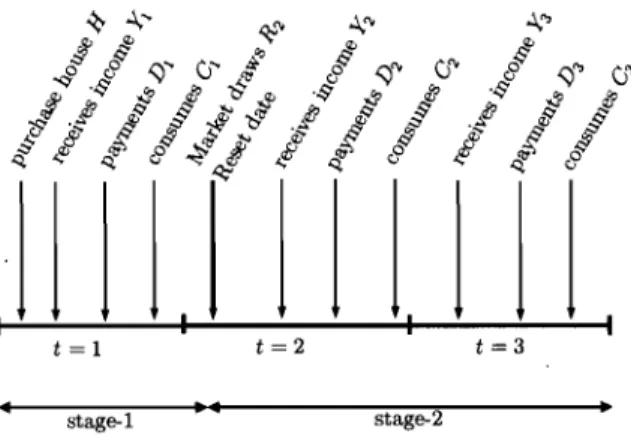
1 1 1 1

t = 1 t=2 t=3

stage-l

••

stage-2

FIG. 1.1 - Timing of the events

We assume that the borrower has no access to credit markets. This assumption is intended to tie up the repayment schedule to the borrower's optimal saving path. The exclusive relationship with the lender may be due to the fact that once the borrower takes on a mortgage loan, subsequent borrowing with another lender is compromised. Indeed, given the size of a mortgage loan relative to income, acquiring a house moves the borrower significantly closer to a binding borrowing constraint. Moreover, there is no room for refinancing because the housing priee is fixed so that home equity is always zero at time 1, by assumption. Consequently, a mortgage contract is the only way available to smooth consumption over time.

1.4 Mortgage contracts

In this section, we describe and give a preliminary analysis of fixed-rate and adjustable-rate. mortgage contract. In doing so we introduce the basic elements of the borrower-Iender relationship.

1.4.1

Fixed-rate mort gage contracts

A complete mortgage contract must specify the repayment schedule. Each repayment consists in two components: an interest-repayment on the out standing loan balance, and an "ad-hoc" repayment of the principal (see Appendix 1.1 for details).7 The amortization period and the term are identical and last three periods. Under the condition _R1Y1

+

Y2 ~ R1H, full payment of the mort gage loan prior to the maturity is prohibited We also rule out default on repayments. Mortgage contracts differ on whether periodic mortgage interest (plus principal) payments are fixed or adjustable with respect to interest rate changes. Under FRM contracts they are fixed. The key feature is that the interest-repayment between period 2 and period 3 is calculated with the expected interest-rate

R

2 .

. An optimal FRM contract is the solution to the following maximization problem :

subject to : Dt> 0, for

t

=

1,2,3,

where

f3

is the discount factor, 0

<

f3 <

1. The first constraint is the period-t budget constraint. It states that the borrower's consumption in any period is determined by its income net of the mortgage

7Notice that, sinee payments of the principal are endogenous the optimal mortgage payments Dt need not be equal for ail t.

repayment. The second and third constraints are imposed by the mortgage contract. The

second-constraint states that, in each period, the borrower makes a non-negative mortgage-repayment.

Consequently, borrowing to finance current consumption is prohibited. The third constraint

repre-sents the lender's zero-profit condition. It states that the present discounted value of payments must

equal the mortgage loan value.8

Solving the FRM problem is pretty straightforward. We use the first constraint to substitute

consumption in the objective function. The problem is now to find the optimal repayment schedule

that maximizes the expected utility under the zero-profit constraint. At the optimum, the

last-repayment trivially equals the outstanding loan balance, so that we are left with an unconstrained

maximization problem, that is :

The first-order conditions for an interior solution are:

(1.1)

(1.2)

U nder our assumptions, these conditions are sufficient as well as necessary for an optimum.

Equa-tions (1) and (2) characterize efficient intertemporal smoothing.

For the purpose of the exposition, we will consider the following equivalent problem in the rest

of the paper :

8Payment Dl should not be confused with a downpayment. In fact, we assume that there is no downpayment requirement in the mortgage.

since it is deterministic, the FRM problem is trivially time-consistent, and therefore it is equivalent

to choose D2 in period 1 or in period 2.

1.4.2 Adjustable-rate mortgage contracts

An adjustable-rate mortgage contract has the same components as an FRM contract, namely

the repayment made at the start of each period to the lender. The key feature of an ARM contract

is that the interest-payment between period 2 and period 3 is decided once uncertainty about R2 is

resolved. Consequently, under an ARM contract a full adjustment of payments D2 and D3 is made

at date 2.

An optimal ARM contract is the solution to the foIlowing maximization problem :

for every realized value of R2

Ct

=

yt - Dt

>

0, Dt

>

0, t

=

2,3,

where E is the expectation operator with respect to the distribution of R2 . The important difference

with the FRM problem is that aIl constraints must hold for every realization of R2 .

To solve this problem, we foIlow similar steps as with the FRM problem, namely we replace all

the constraints into the objective function so as to obtain an unconstrained maximization problem

Now, the second maximization operator is important as the subsequent mortgage payments depend on the ex-post interest-rate. Obviously, early resolution of uncertainty is valuable because payments can adjust to the new information (see Appendix A.2). We solve this problem by backward induction. The first-order conditions, for an interior solution, are: given a first-period repayment z, we obtain optimal values of

D;

by solving the following equation :

U'(Y2 -

D;

(z)) (1.3)

for each realization of R2. The optimal first-period repayment then follows from

Moreover, for any two realized interest-rates

m

and ~ with i

i=

j, the following equation must hold

u'(C~)

mu'(CÜ

u'(c4)

R~u'(C4) (1.5)

Equations (3) and (4) characterize efficient intertemporal smoothing just like the FRM contract. In addition, Eq.( 4) shows that under the ARM contract the marginal benefit of future wealth is uncertain, hence, Dl depends on the borrower's optimal exposure to risk as determined by R2D~ for all R2, where D~

=

(RIDI

+

D2 - RIH) ~

o.

Part of this exposure is implicit and positively

related to the housing value; mechanically, RIH is a scale parameter which controls the variance of the random variable R2. The other part is explicit (endogenous) and controlled by the amount of money devoted to repayments in the first-two periods, i.e., (RIDI

+

D2). More specifically, once uncertainty is resolved, the contingent repayment D2 varies according to Eq.(5) so as to keep the

ratio of marginal utilities unchanged across states of the nature (Le.,

ex-post

interest-rates).

We can interpret

Eq.(5)

as a Borch rule for co-insurance between ("individuals" named) period

2 and period 3. Thus, sharing risk in this case essentially means making a contingent "transfer"

D2 from period 2 to period 3. If, for instance, the size of the payment D2 is bigger for high R2s, then R2D~ unambiguously decreases with respect to

R2

(in absolute value). In this case, bigger

transfers from period 2 to period 3 at states where the risk is high, reduce the overall exposure to

risk. Intuitively, the borrower displays sorne

selj-insurance

behavior in this case. However, if the size

of the payment

D2

is lower for high

R2S,

then the overall exposure to risk is increased eventually. In

this particular case, the borrower takes on added risk in order to increase its final wealth. Intuitively,

it displays sorne

gambling

behavior in that he bets that high interest-rates will occur.

In this paper, our goal is to compare WF and WA• In the absence of risk, the borrower is

indifferent between an ARM contract and an FRM contract, Le., WA WF . Away from this trivial

case, however, an ARM contract entails sorne risk which is absent from an FRM contract. However,

it cornes with a larger set of strategies as the borrower can now adjust its payments to the

ex-post

interest-rate. So, it is unclear which contract is optimal

ex-ante.

1.5 Determinants of the mort gage choice

To start, consider the second-stage problem the household faces after the renewal date, that is,

where y~

Y2 +Rl{Z-H)

and

v

is the indirect utility function given the first-period repayment

z,

and the rate of interest

R

2 (possibly equals to R2)' Notice that

pA

features the expected indirect

the mortgage choice is governed by the borrower's attitude towards interest-rate risk as measured

by v's curvature with respect to R2' i.e., V22. When V22

>

Othe household is thought as being prone

to interest-rate risk. When V22

<

0, on the other hand, the household is thought as being averse to

interest-rate risk.

To see it, assume that V22 is uniformly negative. From Jensen's inequality we have that :

Multiplying both sides of the inequality by (3 and adding up u(YI - z), one cibtains :

This last inequality holds for any z, therefore it must hold when taking the maximum operator on

both sides :

maxu (YI - z)

+

(3Ev (z, R2 )

<

maxu (YI - z)

+

(3v (z,

R

2 ) •

z z

From pA and pF, this is equivalent to

We conclude that :

If then

Consequently, the household will choose the FRM contract. The opposite can be shown when

V22

>

0, i.e., WF

<

WA• However, the indirect utility function vis endogenous so that a simple

1.5.1 Borrower's attitude towards interest-rate risk

In this section, we show that the household's attitude towards interest-rate risk is determined by the way this risk is allocated in the second-stage problem. Basically, the second-stage problem is a standard consumptionjsaving problem under certainty, in that given the "income" flow y~ and

Y3, today and tomorrow, respectively, the individu al pursues intertemporal smoothing by borrowing D~, at the (risk-free) interest-rate R2.

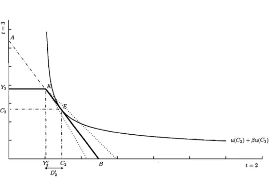
First, we present a geometric treatment. In Figures 2 and 3, we represent the budget constraint when the interest-rate is R2 (line Y3K B) ; and the indifference curve (from the second-stage utility

index) which is tangent to the segment KB. Values of v are drawn from the utility at tangency points (point E), for different combinat ions of

z

and R2 . We are concerned with the welfare effects

of the variability of R 2. With an increase in R2, for instance, the budget constraint pivots clockwise around K so that today's consumption

C2

falls in Figure 2. This happens for two reasons : first, in order to compensate for a relatively cheaper consumption in period 3, so as to keep the same welfare level (substitution effect); and second, because the indebted-household grows poorer (income effect). As for C3 , it decreases as well. Overall, a lower indifference level is attained. However, since a falling

interest-rate brings a welfare gain, the net effect on welfare of the interest-rate risk is ambiguous.

It depends on both the level of the outstanding debt at the beginning of the stage-2 problem and the curvature of the indifference curve. If the out standing debt at the beginning of the second-stage is low enough, then a declining interest-rate increases final wealth, i.e., C3 ; while a rising rate has

no effect on welfare. It follows that dispersion of the interest-rate is welfare-improving provided the indifference curve is curvy enough around E. If such is the case at every level of R2' then the household unambiguously chooses the ARM contract.9

9It should be pointed out that

y;

cannot be too high, in order to in sure that D3 > 0, Le.,

y;

< C2. For c1arity sake, we have just considered the case

y;

> 0, but everything carries on with

y;

negative.

M Il A Y31----..:...t 1 ". "E C3 •. - , _. - , - , - ' _. -.; •••••••••• M Il A B

FIG. 1.2 - Income profile is away from the autarky point

• 1 1· · 1 1· · 1 1· · 1 1· · 1 1· B

FIG. 1.3 - Income profile is around the autarky point

t=2

We can show, rnathernatically, that the household's attitude towards risk depends on the

allo-cation problern in stage-2. From the envelope theorern

then, taking the derivative of V2 with respect to R2 yield

(1.6)

In words, V22'S sign depends on the total effect of interest-rate changes on consurnption levels C2 and

C3. The Slutsky equation describes this total effect. Denote by ft = -u"(Ct}/u'(Ct} the degree of

absolute risk aversion. Total differentiation of the first-order condition Eq.(3) and sorne calculations

(see the Appendix A.4) yields

(1. 7)

which is negative because both the substitution effect - Le., first-terrn in the LHS of Eq.(7)- and the

incorne effect - Le., first-terrn in the RHS of Eq.(7)- are negative. The total effect on C3 , however,

is arnbiguous. To see it, take the first-derivative of the budget constraint with respect to R2 and

notice that 8Dt/8R2

=

-8Ct/8R2, it yields

(1.8)

The sign of the substitution effect on C3 is the opposite of 8C2/8R2, while the sign of the incorne

effect is the sarne, that is, C2 and C3 are normal goods. Overall, C3 increases when the substitution

at this specifie R2. If this is true for an realized values of R2, then the borrower always chooses

the ARM contract. For the indirect utility function to be concave, however, it is necessary that

8C3/8R2 be negative; that is, the income effect dominates the substitution effect on C3.

One can show that : if the borrower does not earn enough income in the first-two periods to pay

off its entire loan, and if its elasticity of substitution is uniformly lower than one; then 8C3/8R2 ~ 0

everywhere (see Lemma 1, in the Appendix 1.5).

Condition 1. _R1Y1

+

Y2 ~ RIH and Vt ~ 1 for ail

t.

Under Condition 1, V22'S sign is ambiguous. Hence, it guarantees that the borrower won't choose

either ARM or FRM for all parameter values (as it would be the case if V22

< 0 or

V22

> 0). It will

de pend on the elasticity of substitution and the outstanding debt in the second-stage.lO To see it,

rewrite Eq.(8) as follows

(8')

where Vt

=

-Ctu" (Ct) lu' (Ct) represents the inverse of the elasticity of substitution (and the degree

of relative risk aversion). The sign of the numerator de pends on both the elasticity of substitution

and the size of last-period repayment relative to consumption in period 2. The lower the elasticity

of substitution, or the higher the ratio of last-period repayment to second-period consumption, the

more likely 8CJ/8R2 is negative. Obviously, it happens away from the autarky point (see Figure 3).

80 far, we have just considered the stage-2 problem for isolated value of R2. The design of

payments D2 and D3 contingent on the realized interest-rate has important implications for the

exposure to risk under the ARM contract. The borrower displays sorne self-insurance behavior when

the income effect dominates the substitution effect everywhere. Although, the optimal exposure to lONotice that Y~ is negative under Condition 1.

risk does not have to be zero, because renouncing to consumption in period 2 (and period 1) is costly

in terms of marginal utility, doing so brings positive return in expectation. Under Condition 1, the

borrower can find optimal to choose the ARM contract while at the same time insuring himself.

However, in the limiting case where it is too costly to renounce to consumption (i.e., too costly to

insure himself), the borrower will find optimal to choose (the full insurance of) an FRM contract.11

On the other hand, when the substitution effect dominates the income effect everywhere, the

borrower displays sorne gambling behavior. Choosing the ARM contract is thus unambiguously

optimal. 12

1.5.2 Borrower's allocation of risk over time

In this section, we study the role of the first-period repayment in the mortgage choice. With

a bigger first-period repayment, for instance, a lower debt burden is carried into the second-stage.

This affects the autarky point, and thus the mortgage choice.

In the stage-l problem, the borrower decides consumption, and savings, which proceeds become

available for consumption in period 3.13 However, unlike the FRM contract, first-period saving under

the ARM contract is subject to uncertai nty. So, comparing first-period repayment under the two

contracts is similar to asking : how, starting from a zero-risk situation, an increasing risk affects

saving under the ARM contract. We distinguish two channels : first, increasing risk translates into a

higher return on savings in the stage-2 problem, for each state ; second, increasing risk exogenously

alters the exposure to risk from the standpoint of the stage-l problem.

Let us parameterize the risk as

R2

=

R2

+

1]€, where € is a zero-mean random variable, 1] is

HIf Vt is high enough.

12The amount invested in R2 is similar to a short position in a risky asset.

a positive scale parameter, and the support of é is such that

R

2

+

"lé is no less than one.14 For

instance,

R2

+

"lé could describe a family of uniformly distributed random variables, all having a mean equals to

R2'

with variance parameterized by "l. The FRM problem is obtained by"l

=

o.

A small increase of"l from zero, constitutes a MPS (mean preserving spread) shi ft of the distribution

of R2. Combining Eq.(3) and Eq.(4), and differentiating it with respect to "l, we obtain :

(1.9)

where D is the second-or der condition of the ARM problem

with 8C3/8"l given by Eq.(8).15

An increased riskiness has two effects on the first-period consumption. A direct effect - i.e.,

first-term in the brackets of Eq.(9)- which follows from changing the dispersion of the return from

saving around the mean. Since u'(C3 ) is uniformly increasing with respect to é, the sign of the direct

effect depends solely on the sign of 8C3/8é; which is the same as 8C3/8R2'S sign. When the income

effect dominates the substitution effect everywhere, i.e. 8C3

/&

::S; 0 for all R2' the direct effect is

negative. In turn, first-period consumption tends to fall as the borrower needs additional resources

in the second-stage problem for the Euler equation Eq.( 4) to hold. Graphically, if all tangency

points lie around the autarky point, as in Figure 2, a higher dispersion moves them away from it

by rotating the budget constraint clockwise for each initial R2. Hence, by increasing first-period

repayment, y~ is reduced so that tangency points still lie around the autarky point. On the other

hand, when the substitution effect dominates the income effect everywhere, i.e. 8C3/8é

>

0 for all 14Davis (1989) considered a similar parameterization.

R2' the direct effect is positive. Notice that, risk aversion alone suffices to sign this effect.

Furthermore, an indirect effect - Le., second-term in the brackets of Eq.(9)- follows from carrying

sorne risk. Under prudence, for instance, if it is optimal to hold a non-zero risk then individuals tend

to increase saving in the face of uncertainty. While risk aversion defines an individual's attitude

toward uncertainty, prudence defines how an individual reacts to it. Leland (1968) and Sandmo

(1970) first formalized this concept and proved that a convex marginal utility, Le. ulfl

>

0, is attached to such a prudent behavior.16 _{Later on, Kimball (1990) introduced the degree of absolute}

prudence, defined as <Pt _{-ulll(Ct)/U"(Ct ).} In our setup, the analysis of the precautionary effect

is complicated by the fact that payments adjust to the realized interest-rate. To see it, notice that

the indirect effect is negative if the derivative of R2(8C3/8ry)UI/ (C3) with respect to e: is uniformly

positive. The computation of that derivative yields the following expression:

[ 8C3 R 8 2

C3] Il (C) R 8C3 8C3 f/f (C ) ry 8ry

+

2 8ry8e: u 3

+

2 8ry 8e: u 3

which is a weighted sum of second- and third-derivatives of the utility function. The weight on

UIfl

(C3) is positive since it has the same sign as (8C3/8R2)2. It follows that if 8C3/8ry is

inde-pendent of e: (Le., _{8 2C3/8ry&} = 0), and if the risk is small (Le., ry ~ 0), then the indirect effect is

negative provided that prudence (i.e., <P3) is sufficiently high. In this case, the indirect effect can

unambiguously be termed as the precautionary effect.

When payments adjust to the realized interest-rate, however, 8C3

/Bry

is no longer independent

of e: (Le., 82C3/8ry&

f:.

0). Consequently, the precautionary effect should now reftect the

endo-genous change in the exposure to risk. More specifically, a positive weight on ul/(C3 ) reduces the and Modigliani (1972) generalized Leland and Sandmo's results to non-additively-separable utility func-tions.

precautionary effect, while a negative weight reinforces it. The quantity Ô2C 3/Ô1}Ôé measures the marginal change in the exposure to risk, as a result of allocating the risk between period 2 and period 3. Obviously, it depends on the dynamic of both substitution and income effects, but we are not aware of any theoretical result on this dynamic. Under Condition 1 and for a iso-elastic utility specification, Ô2C3/Ô1}Ôé is positive (see Appendix A.4). Intuitively, self-insurance reduces the car-ried risk so that the precautionary effect is weakened. In general, the total effect is ambiguous. In the Appendix A.5, we show that for the total effect to be negative, it suffices that V122 be uniformly positive (see Lemma 2).

1.6 Mortgage choice with constant relative risk aversion

This section aims at clarifying aIl ambiguities in the model by drawing qualitative results based on CRRA preferences. This preference class is standard in finance and macroeconomics, and most importantly is consistent with realistic consumption patterns under uncertainty as opposed to say CARA or quadratic preferences. 17

Consider the constant relative risk aversion (CRRA) utility function of the form :

u(C)

=

(Cl-II - 1)/(1 - Il), for Il

>

0,

where Il is the degree of relative risk aversion, and Il

+

1 is the degree of relative prudence. With··

this specification, it is readily verified that the optimal co nsum pt ion plan under the FRM contract can be described as follows :

t=1,2,3,

17In a similar three-period framework, Blundell and Stocker (1999) examine the impact of incorne risk on consump-tion patterns, when the timing of the resoluconsump-tion of uncertainty varies. They conclude that "the preferences of the

eRRA class [are] perhaps the most realistic for modelling actual saving behavior in empirical work, because they can capture the most plausible precautionary behavior for rich and poor households."

Y2 Y3 F - [ - 1/ - - 1/ ] F F 1/

where

w

= Y1

+

R1

+

R1R2'

al

= (R1 R2)/ R1R2

+

({3R1) I/(R2

+

({3R2) 1/),

a

₂ =

al

({3R1) 1/ and

a:

=

a;

_({3R2) 1/1/. Typically, the borrower uses the FRM contract to allocate fixed shares of its lifetime's net wealth to consumption in each period. In fact, any change in the timing of the income profile that leaves the wealth level unchanged, will also leave the consumption profile unaffected. Under the ARM contract on the other hand, no closed-form solution is available for the entire consumption profile. But, we can still obtain the consumption plan of the second-stage problem, that is :

t

=

2,3

net wealth is allocated to C2 and C3 , respectively. However, the timing of the income profile becomes

relevant for the first-period consumption because it is affected by uncertainty. We will compute C: numerically.

1.6.1

The effect of uncertainty

To single out the borrower's reactions toward risk, we use as benchmark the fixed-rate mortgage problem when the borrower does not use the mortgage contract to smooth consumption but simply to access homeownership.

In terms of parameters, it me ans setting {3R1

=

{3R2 = 1 and

Yt

=

y for all t, so that the agent has no incentives to borrow or save, and the consumption profile is fiat and independent of v. For the remainder of the section, we will use Y

=

2 and {3 = 0.8 unless stated otherwise. The future interest-rate is assumed to be R2 = R2

+

'riE, where E is uniformly distributed over the interval

[-€,€l

and discrete on a grid of 11 points, with 10

=

R2 - 1 (so that the lower bound is no less than

R

2 by increasing ry. We execute this experiment, numerically, for several degrees of risk aversion and

housing values.

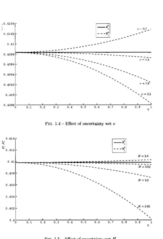
From Figure 4, it appears that, in absence of risk (Le., ry = 0) the first-period shares are equal under the two contracts. Unlike first-period shares under the FRM contract,

0:

is affected by both the increasing risk and the changing parameter v.18 _{For low values of risk aversion, the}

borrower gambles on interest-rate, that is, the direct effect is positive. Moreover, it dominates the precautionary effect so that the borrower enjoys additional risk to the extent that wealth is sent to the risk-free period 1. In this case, first-period share increases with respect to risk, and is greater than its counterpart in the FRM contract everywhere. At higher degrees of risk aversion, the borrower eventually stops gambling and the direct effect bec ornes negative. In addition, since the degree of prudence is increased as well, the precautionary effect reinforces the direct effect so that the borrower sends much wealth into risky periods in order to insure himself.

From Figure 5, it appears that raising the housing value H generates the same reactions towards risk as raising v. In fact, by increasing the overall indebtedness, a higher housing value makes gambling on high interest-rates less attractive, consequently the direct effect goes from being positive to being negative. In the meantime, a higher H increases the implicit risk exposure so as to raise the optimal exposure to risk and thus the precautionary effect (everything else being equal, specially

v, ry and €'s variance). Overall,

0:

is increases at first with respect to risk for low values of

H,

and then decreases for higher values.

Based on Figures 5 and 6, we conclude that the substitution effect dominates the income effect for low values of H, or low values of v, while the income effect dominates the substitution effect for high values of H, or high values of v.19 _{In Figure 6, we provide additional support about}

18The share is computed as e~ =

c:

j(w - H), we use it in order to eliminate level effects.

.0.4104 0.4102 0.41 0.4098 0.4096 0.4094 0.4092 0.409 0.4088 0 0.1 0.414

~-"'.

,-'"

0.412 0.41 0.408 0.406 0.404 0.402 0.4 0 0.1

---

---R

U

--- --

--v

0l _ .

--=====::--:---

-...

----

... 0.2 ... "" ... ~~~ 0.3 0.4 0.5 0.6 0.7

..

_..

_..

0.8

FIG. 1.4 - Effect of uncertainty wrt 1)

R

U

.. ..

v L3 v " " 11

.. ..

2.5 0.9 ... _... 1 11 H=2.6

---

....

---

---... .;.. .... - - - - .... - .... .... H = 3.05

---

....

_-

.... ~-~ ~~~ ~~~ H=3.5 ... _...

_..

...

..

... ... ... ... ,H =3.95 ...

_,

...

_...

...

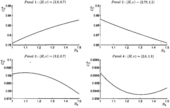
0.2 0.3 0.4 0.5 0.6 0.7 0.8 0.9 1 11

the dynamics of both effects with respect to the housing value and the el asti city of substitution, respectively. Let us first set Ti

=

1. We then give an illustration of each possible configuration of 03

over the interval of R2. Panels 1 and 2 depict the cases where 803/8R2 keeps the same sign over the interval of R2, these cases are well understood (Panels 1 and 2 are obtained for the combination

H = 2.9, /1 = 0.7, and H = 2.75, /1 = 1.1, respectively). Computations suggest that the total effect

of risk on first-period consumption is dominated by the direct effect. Panels 3 and 4 depict hybrid cases where _{803/8R2 changes sign over the interval of R2 (Panels 3 and 4 are obtained for the} combination H = 3.2, /1 = 0.7 and H = 2.6; /1 = 1.1, respectively).2o In Panel 3,03 first increases, and then decreases. In Panel 4, 03 first decreases, and then increases. We summarizes these finding

as follows :

Consider a borrower with a constant degree of relative risk aversion. Then, he finds optimal to choose the ARM contract : (i) if he is not too averse to risk; or

(ii)

if the housing value is not too high.

Starting from a situation where the borrower is indifferent between an ARM contract and a FRM contract, a borrower with a lower degree of risk aversion requires less insurance than what the FRM contract offers, so that he would rather self-insure and bear sorne risk in exchange for additional wealth. From the same initial situation, a borrower with a lower housing value faces less implicit risk while has more revenues early on to speculate on future interest-rates. He thus needs less insurance than what a FRM contract offers so that he finds optimal to choose the ARM contract. We illustrate Proposition 1 in Figure 7 (in Appendix A.5, we report sorne numerical result

equivalent to a CES utility function with elasticity of substitution equal to 1/1/ (this intuition is due to Larry Epstein (1980)). As such, we recall that, C2 and C3 are complements when 1/ > 1, and perfect complements (Leontief) in the

limiting case 1/ - -00. They are substitutes, on the other hand, when 1/ < 1, and perfect substitutes in the limiting

case 1/ -- O. In our setup, the budget constraint (income effect) makes this classification depend on other parameters as weil. Geometrically, it has to do with the fact that preferences of the CRRA-class are (quasi)-homothetic and that the curvature of the contour of a typical indifference curve is controlled by a single parameter, i.e., 1/.

20These cases are rather scarce, for 100 combinations of H and 1/ we found just the two cases that appear in Panels 3 and 4, respectively.

Panell: (H,v) = (2.9,0.7) 0,86 0,84 0,82 0,8 0,78L.---~---'---... -:", 0.7 Q 0.695 0,69 0.685 0,68 1 1.1 1,2 1.3 1.4 1.5 R2 Panel 3: (H,v) = (3.2,0.7) 0.675'---~--~--~---'--"'" 1 1.1 1.2 1.3 1,4 1,5 R2 Pane! 2: (H, v) (2.75,1.1) -: 0,9

cS

t'

0.89 °,86,' - - - - , .... , - -...

,.-2--, .... 3---,.4--... ,.5

R2 Panel 4 : (H,v) = (2.6,1.1) 0,9365 0.936 0.9355 0.935 0.9345 °,934 ,'----, ... , , - -... ,.~2--, ... ,3---,.4--... ,.5 R2

FIG. 1.6 - Last-period consumption wrt to interest-rate

H

o v

FIG. 1.7 - Mortgage choice, housing value and relative risk aversion