Eulerian model of immersed elastic surfaces with full membrane elasticity
Texte intégral
Figure


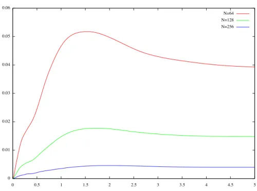
![Fig. 5.6: Vertical radius up to t = 30 (Top). Zoom on t ∈ [0,5] for N = 64, 128, 256.(Bottom)](https://thumb-eu.123doks.com/thumbv2/123doknet/7292104.208442/19.918.136.640.143.888/fig-vertical-radius-t-zoom-t-n.webp)
Documents relatifs
For each bud, computation of the preformed growth unit: calculation of the number of metamers according to the ratio between biomass and demand, and
Dans ce travail, en utilisant les premiers principes ; la méthode d'ondes planes linéarisées à potentiel complet (FP-LAPW) basée sur la Théorie Fonctionnelle de
L’accès à ce site Web et l’utilisation de son contenu sont assujettis aux conditions présentées dans le site LISEZ CES CONDITIONS ATTENTIVEMENT AVANT D’UTILISER CE SITE WEB.
This binding event is characterized mainly by a change (increase) in mass that cannot be solely explained from the peptide weight itself (as it could not lead to such large
Our purpose is to derive rigorously the Helfrich energy W µ as a limit as ε goes to 0 of a 3-D nonlinear elasticity theory for vesicle membranes with small but positive thickness
We first restrict to the case of small initial data (n ≥ 2), and use a variant of the Picard fixed point theorem as in the proof of Kato’s and Chemin’s theorems for the
Full-circle Eulerian cradle for low temperature neutron
