BAROTROPIC PREDICTION OF 500-MB AND 100-MB FLOW PATTERNS
by
HAROLD M. WOOLF
S.B., Massachusetts Institute of Technology (1960)
SUBMITTED IN PARTIAL FULFILLMENT OF THE REQUIREMENTS FOR THE DEGREE OF
MASTER OF SCIENCE
at the
MASSACHUSETTS INSTITUTE OF TECHNOLOGY June, 1961
Signature of Author
...-...
- -... .Department/ of Meteorology, May 20, 1961
Certified by....
Thesis Supervisor
Accepted by. .. . . . ...
...-Chairman, Departmental Committee on
/
Gr aduate Students IASI. OF TECHN 0JUN 19 1961
LJBRAFVBAROTROPIC PREDICTION OF 500-MB AND 100-MB FLOW PATTERNS by
Harold M. Woolf
Submitted to the Denartment of Meteorology on May 20, 1961, in partial fulfillment of the requirements for the degree of Master of Science.
ABSTRACT
Vertical profiles of mean zonal wind component at 30, 40, and 50 degrees North Latitide imply that the equiv-alent-barotropic levels defined by Charney and Eliassen (1949) are located between the 500-mb and 400-mb levels, and very near the 100-mb level. An investigation was carried out in order to ascertain whether or not 100-mb flow behaves, and can be predicted, barotropically. The equivalent-barotrooic prognostic equation was inte-grated numerically on the IBM 709 computer. Forecasts were made for periods of 24 and 48 hours during an
act-ive situation, for 500 mb as well as 100 mb to provide a basis for comparison of results.
The results of the numerical prediction indicate that while the 100-mb forecast errors are small, a lower deg-ree of forecast skill is displayed at that level than at 500 mb. In every forecast period the barotropic tech-nique predicted excessive eastward displacement of the 100-mb trough. A field of large-scale divergence, which would be neglected in the equivalent-barotropic proced-ure, was postulated as the source of this systematic error. Supplementary computations were performed, and a plausible hypothetical divergence pattern was deduced therefrom.
The value of the 100-mb prognostic charts in wind forecasting was also investigated. Geostrophic winds determined from these charts yielded root-mean-square vector errors substantially smaller than the errors in
persistence forecasts, for periods of both 24 and 48 hours. However, in view of the small data-sample ob-tained, it was concluded only tentatively that the meth-od presented is a generally useful and valuable 100-mb wind-prediction technique.
With respect to both the barotropic-prediction and wind-forecasting phases of the investigation, it was concluded that considerable additional study is both necessary and desirable.
This thesis was done in part at the MIT Computation Center, Cambridge, Massachusetts.
Thesis Supervisor: Frederick Sanders Title: Associate Professor
ACKNOWLEDGMENT
To Prof. Frederick Sanders of the MIT Meteorology Department, who as thesis advisor provided many helpful suggestions and much encouragement during the course of this project, the author wishes to express his sincere appreciation.
The author is grateful to Mr. Sidney Teweles of the United States Weather Bureau for providing the 100-mb analyses used in this thesis.
The services of Miss Leola Odland, Meteorology Depart-ment programmer, and of the staff and facilities of the MIT Computation Center are also appreciated.
The assistance of Mr. A. James Wagner in analyzing several of the charts presented in this report is grate-fully acknowledged.
Special thanks are due to Miss Isabel Kole for prepar-ing the many figures for publication.
TABLE OF CONTENTS
Section
I. INTRODUCTION
II. THEORETICAL DISCUSSION
A. Equivalent-Barotropic Vorticity Equation B. Determination of Equivalent-Barotropic
Levels
III. PREPARATION OF PROGNOSTIC CHARTS A. The Initial Synoptic Situation B. The Computational Procedure IV. RESULTS OF BAROTROPIC PREDICTION
A. Presentation B. Discussion
C. Application to Wind Forecasting V. SUMMARY AND CONCLUSIONS
APPENDIX REFERENCES Page 9 10 10 12 14 14 14 16 16 16 38 42 45 50
FIGURES AND TABLES
Figure Page
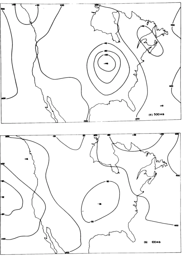
1. Observed heights, 1200 GCT 18 November 1957. 17 2. 24-hour barotropic forecasts for 1200 GCT
19 November 1957. 18
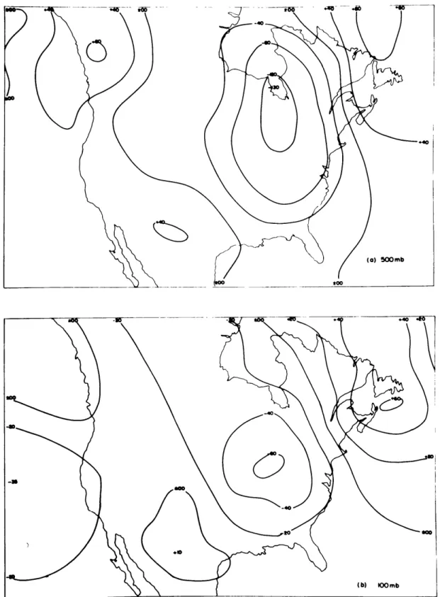
3. Observed heights, 1200 GOT 19 November 1957. 19 4. Observed 24-hour height changes, from 1200
GOT 18 November to 1200 GOT 19 November. 20 5. 24-hour-forecast errors, 1200 GOT 19 November. 21 6. 48-hour barotropic forecasts for 1200 GOT
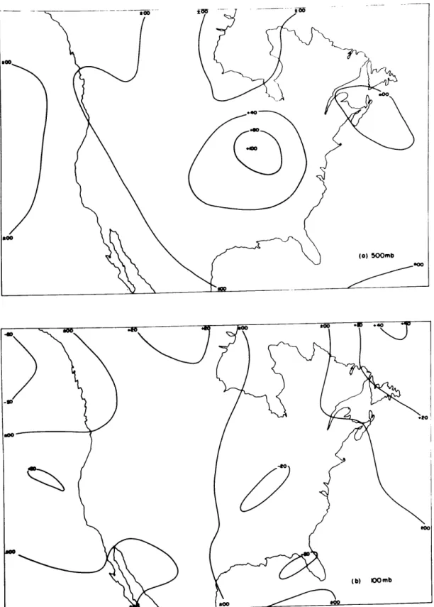
20 November. 22
7. Observed heights, 1200 GOT 20 November. 23 8. Observed 48-hour height changes, from 1200
GOT 18 November to 1200 GOT 20 November. 24 9. 48-hour-forecast errors, 1200 GOT 20 November. 25 10. 24-hour barotrooic forecasts for 1200 GOT
20 November. 26
11. Observed 24-hour height changes, from 1200
GOT 19 November to 1200 GCT 20 November. 27 12. 24-hour-forecast errors, 1200 GOT 20 November. 28 13. 100-mb "divergence" patterns (unit 10-6sec-1)
determined from ten-lemodel vertical
Figure 14. MachinE SmOOthE (unit 1 1200 GC 15. Diverge produce
FIGURES AND TABLES (contd.)
-computed (a) and subjectively d (b) absolute vorticity patterns 06 sec -) associated with trough, for
T 18 November 1957.
nce (unit 10-6 sec~ ) required to derived D-values. Table 1. 2.
3.
A 1. A.2.CONTRIBUTIONS TO TROUGH-LINE SPEED
CONTRIBUTIONS TO TROUGH-LINE SPEED AS COM-PUTED FROA SMOOTHED VORTICITY
100-mb WIND FORECAST RESULTS
VERTICAL WIND-SPEED PROFILES, DETERMINED GEOSTROPHICALLY BETWEEN 70W and 125W VERTICAL WIND-SPEED PROFILES, DETERMINED
FROM BUCH'S HEMISPHERIC WIND DATA
Page
35
36
34
36
39
46
SYMBOLS
x east-west horizontal coordinate y north-south horizontal coordinate p pressure, vertical coordinate
t time
Z geopotential height of a constant-pressure surface \V horizontal wind velocity vector
\Vnd non-divergent part of horizontal wind vertical comoonent of relative vorticity
f coriolis parameter, 2.Q sin 0 , where ...
=
angular velocity of the earth, = latitudef "standard," constant value of f, equal to 10~4sec~ (A) vertical "velocity," do
A(p) equivalent-barotropic modeling coefficient
( )G value of ( ) at the surface of the earth u mean zonal wind
I. INTRODUCTION
The equivalent-barotropic model, proposed by Charney and Eliassen (1949), was the first numerical weather pre-diction scheme to be tested by means of high-speed digital computers, and according to Ellsaesser (1960) has been in operational use by the Joint Numerical Weather Prediction Unit since 1956. It has been applied, in research as well as in routine forecasting, principally to flow at the 500-mb level. Certain theoretical considerations, which are
related in the following section of this renort, led the author to believe that significant results might be ob-tained by barotropic prediction of flow at 100 mb. As a by-product of the purely scientific interest of the prob-lem, namely the investigation of the computational conse-quences of a theoretical proposition, an engineering apoli-cation was realized--the use of a 100-mb prognostic chart, once obtained, as an aid to wind forecasting. The predic-tion of winds at the 100-mb level, at an altitude of approx-imately 16 km, is certainly a practical problem, for mili-tary aviation at present and for commercial operations in the not-too-distant future. While the major effort in this study has been devoted to the portion of the problem of greatest scientific interest, consideration has been given to the engineering aspect as well.
II. THEORETICAL DISCUSSION
A. Equivalent-Barotropic Vorticity Equation
Phillips (1958) has presented a clear and concise devel-opment of the prediction equation for Charney and Eliassen's (1949) model. The starting point is the vorticity equation in (x,y,p,t) coordinates, exact except for the assumption of hydrostatic equilibrium and the neglect of friction:
--
\'
~_+
-
5
(4
+ t 7 f --- --
3----u ,1
Dt
a
P
'3X
9 P
?.Y 'P
If the geostrophic approximation is made, Charney's (1948) scale considerations permit one to simplify Eq. (1) to a great extent by neglecting terms that are one or more orders of magnitude smaller than the principal terms of the equa-tion. By also making use of the (x,y,p,t) form of the equa-tion of continuity
V'\V
-
=
0
(2)
one may then write the simpler vorticity equation
The fundamental modeling approximation is twofold: firstly, the direction of the non-divergent part of the wind is invariant with, or independent of, height or
pres-sure above a given point; secondly, the same vertical pro-file of non-divergent-wind speed is valid at all points (x,y,t). The simple mathematical expression of this rela-tionship is
\V,
A
\\/'Id
(X )
(4)where
( )
- -- ( )dp, the average with respect to pressureof the quantity ( ). It is obvious from Eq. (4) that A = 1. Substitution of Eq. (4) into Eq. (3) gives
nd.9
+
A
6
-
,(5)
Pressure-averaging or "barring" of Eq. (5) yields
Let \V* = A \Vnd, hence A . Then Eq. (5a) can be
written-\ -+.. ' (6)
P6
-U---Except over strongly sloping terrain, the last term in Eq. (6) can be neglected, leaving the equivalent-barotropic vorticity equation in its simplest form:
0)+
(7)
which states that the absolute vorticity is conserved follow-ing the horizontal motion at the "star" level(s), where A=A This is the form of the equation emoloyed in the present in-vestigation.
B. Determination of Equivalent-Barotropic Levels
The equivalent-barotrooic or "star" levels in the at-mosphere can be determined from actual wind data, or if the
geostrophic approximation is made, from isobaric height data. Buch's (1954) northern hemisphere mean winter wind data indi-cate that at 30, 40, and 50 degrees North Latitude, A= At between 500 mb and 400 mb, and slightly above 100 mb (see
Table A.2). This fact led the author to initiate this study, in order to determine whether or not flow at the 100-mb level behaves barotropically.
For the case studied in this project, the equivalent-barotropic levels were determined geostrophically for 30, 40, and 50 degrees North Latitude, between 70 and 125 degrees
West Longitude (see Table A.1), at the initial time of the forecast period, 1200 GCT 18 November 1957. The results show the levels to be almost exactly at 100 mb, and near 400 mb. The two levels for which forecasts were made are 100 mb and 500 mb; the effect of making a barotropic fore-cast for a non-barotropic level is discussed in a later section of this thesis (see Section IV., Part B.).
00,00
III. PREPARATION OF PROGNOSTIC CHARTS
A. The Initial Synoptic Situation
The most prominent feature of the situation, and the one of greatest interest for the subsidiary
wind-forecast-ing study, is the deep trough (hemispheric wave number six) located over central North America (see Figs. 1, 3, 7).
While there are other features of interest on the initial maps (Fig. 1), forecasts of their future behavior were ex-pected to be quite poor, principally because of the boundary
constraints. Further comment on this point may be found in Section IV., Part B.
The situation was studied for a 48-hour period, from 1200 GOT 18 November 1957 to 1200 GOT 20 November.
B. The Computational Procedure
The prognostic calculations were performed on the IBM 709 Electronic Data Processing Machine of the MIT Computa-tion Center. The program had been previously prepared by members of the Dynamical Forecasting Project 3f the MIT Meteorology Department. Input information consists of iso-baric height values in decafeet on a rectangular grid of 486 points (27 x 18), with diagonal grid-point separation of five degrees of latitude, or 300 nautical miles.
-. -- r
WV-The simple equivalent-barotropic vorticity equation (Eq. (7)) is transformed into the finite-difference analog of a Poisson equation, which is then solved by relaxation for the local rate of change of isobaric height,
dZ/?t.
Iterative integra-tion in time (A4t=
45 minutes) yields predicted height values which then become the initial data for a new Poisson equa-tion. The relaxation-iteration orocedure continues until the end of the desired period, whereupon the forecast height val-ues in decafeet are printed out by the computer. The valval-ues were transcribed to a grid overprinted on the standard MIT Meteorology Department North American Base Map, and analyzed in the usual fashion.Forecasts were made for both levels under study for periods of 24 and 48 hours with 1200 GCT 18 November as the initial time, and for 24 hours with 1200 GCT 19 November as the initial time.
The computer program also yielded grid-point values of absolute vorticity at each print-out stage, which though not displayed in Section IV., Part A., proved to be of value for supplementary calculations presented and discussed in Part B. of Section IV.
IV. RESULTS OF BAROTROPIC PREDICTION
A. Presentation
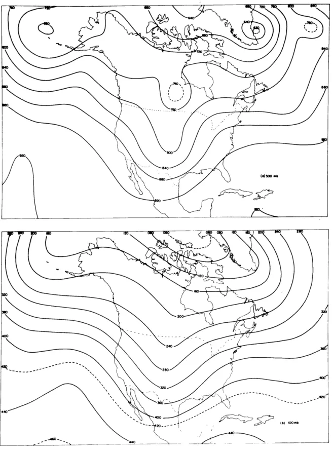
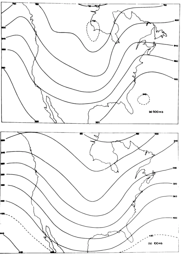
In the figures on the following twelve pages are pre-sented charts of initial, forecast, and observed isobaric height patterns, observed height change, and forecast error
(predicted minus observed) patterns for all of the initial and verification times and forecast periods of the case.
The upper portion of each figure, designated (a), refers to conditions at the 500-mb level; the lower portion, designated
(b), to 100 mb. All contours are labeled in tens of feet; on the isobaric height maps, the tens of thousands digits are omitted, following conventional meteorological practice. The omitted digits are one for 500 mb and five for 100 mb.
B. Discussion
Some qualitative assessments of the probable "goodness" of the various forecasts were made before the actual prog-nostic computations were performed. Solution of the finite-difference Poisson equation by relaxation on a rectangular grid requires arbitrary specification of boundary values;
it has been general practice in problems of this nature, followed in the computer program used in the preparation of the material presented here, to fix the initial boundary height values for all time. It was therefore expected that
Figure 1. Observed heights, 1200 GCT 18 November 1957.
Figure 2. 24-hour barotropio foreoasts for 1200 GCT 19 November 1957.
.igure 3. Observed heights, 1200 GCT 19 November 1957.
~q I
w-Figure 4. Observed 24-hour height changes, from 1200 GCT 18 November to 1200 GCT 19 November.
Figure 5. 24-hor-forecast errors, 1200 GOT 19 November.
Figure 6. 48-hour barotropic forecasts for 1200 G3T 20 November.
Figure 7. Observed heights, 1200 GCT 20 November.
--I
Figure 8. Observed 48-hour height changes, from 1200 GCT 18 November to 1200 GOT 20 November.
i
Figure 9. 48-hour-foreoast errors, 1200 GCT 20 November.
(a) S00mb
.400
Figure 11. Observed 24-hour height changes, from 1200 GOT 19 November to 1200 GOT 20 November.
large and unrealistic errors in prediction would be evident within two or three grid-points of each boundary. The major trough over central North America, except for its southern extremity, is well within the remaining "non-boundaryu re-gion, and the prediction of its development was not expected to be affected noticeably by the boundary constraints.
It has been mentioned above (Section II., Part B.) that the lower equivalent-barotropic level over the area of con-cern is 400 mb, while the oredictions are made for 500 mb. The u and A profiles presented in Table A.1 indicate that the values of u, and hence of A, are greater at the 400-mb level
than at the 500-mb. From this fact one would expect a por-tion of the forecast error at 500 mb to be due to an under-estimate of the eastward displacement of the trough.
According to Sanders, Wagner, and Carlson (1960) the first 24 hours of the case were a period of rapid develop-ment througnout the troposphere over central North America
in association with the deepening of an intense sea-level cyclone. The mid-tropospheric height changes of the second 24-hour period, on the other hand, were essentially baro-tropic in character. It was then concluded that in broad
terms the first 24-hour 500-mb forecast would be rather poor, with predicted heights much too high over a large area; the 48-hour, as bad or worse; and the final 24-hour prognosis, the most promising of the entire series.
On the basis of Charney's (1949) and Hinkelmann's (1953) conclusions regarding the propagation of disturbances in the vertical and the vertical extent of influence regions
significant for dynamical prediction, it was expected that the 100-mb flow would be affected slightly or not at all by the intense baroclinic development occurring in the tropo-sphere. No other possible sources of forecast error at 100 mb were suggested prior to the actual preparation of the prog-noses.
The maps presented in Part A. of this section corrobor-ate the foregoing assertions to a high degree. On the first two 500-mb prognostic charts (Figs. 2(a) and 6(a)) and the corresponding error maps (Figs. 5(a) and 9(a)) the effects of prediction of insufficient trough displacement and of fail-ure to predict the intense development are readily apparent. The lagging of the trough is still in evidence on the second 24-hour forecast map (Fig. 10(a)) and its accompanying error field (Fig. 12(a)), but the actual deepening of the low center was forecast nearly perfectly.
The height changes at 100 mb, as proposed above, reflect essentially no influence of the lower-level baroclinic devel-opment. Rather, the errors obtained in barotropic predic-tion of the 100-mb flow, as one may readily deduce from the prognostic (Figs. 2(b), 6(b), and 10(b)) and error (Figs. 5(b), 9(b), and 12(b)) maps, are attributable primarily to
--.-
-casts of excessive eastward displacement of the trough. The
existence of a field of large-scale divergence, positive ahead of the trough and negative (convergence) behind it, was suggested as a oossible explanation of this phenomenon.
The author was fortunate to have access to computations made with a ten-level numerical model on the same situation, for
the study by Sanders, Wagner, and Carlson (1960) cited previ-ously. One of the products of the machine program is a
com-olete set of grid-point vertical velocities (a)) for each of
-4 -1
the ten levels, 100 through 1000 mb, in units of 10 mbsec . With the assumption of the boundary condition A), MO, the finite-difference approximation to the equation of continuity (Eq. (2)) may be written
(M.
\V
=
&
z
-
L
00
'
/
-
M
b
(8)
providing a rough estimate of 100-mb divergence. It is only a crude approximation because the vertical motions above 200 mb, while small in magnitude, are highly variable. How-ever, the approximation was considered adequate for the en-suing discussion. Patterns of "divergence" so determined are shown in Fig. 13, for the two times for which the ten-level-model results were available.
Computations were made to assess the magnitudes of the contributions of gradient of vorticity advection and gradient
Figure 13. 100-mb "divergence" patterns (unit 10-6se0 1)
determined from ten-level-model vertical velo-cities (dashed line - trough line on the 18th; dotted line - trough line on the 19th).
of divergence to abetting and/or retarding the eastward move-ment of the vorticity pattern associated with the trough.
The kinematical equation for the speed of the axis of the vorticity pattern, by analogy to Petterssen' s (1956) formula for the sneed of a pressure-trough axis, is
(9)
932
where the x-axis is oriented normal to the vorticity-pattern axis, henceforth denoted "trough line" for convenience.
Substitution for from the vorticity equation (Eq. (3))
gives the formula
....
(10f)
The derivatives in Eq. (10) were approximated by finite dif-ferences and evaluated numerically with the grid-point values of 100-mb height and absolute vorticity for 1200 GCT 18 Nov-ember provided by the barotropic computer program, and those of determined from the ten-level model vertical velocities. For the sake of brevity the first term in the numerator of
the right-hand side of Eq. (10) will hereafter be referred to as "V," while the second term will be designated "D."
During the first 24 hours of the case the actual speed of the trough line was 8.8 knots, while the barotropically
33
v-predicted speed was 17.6 knots. If this difference between predicted and observed speeds were indeed due to the neglect
of divergence, then at a given point on the trough line the value of V should be exactly twice that of D.
Values of V, D, and C computed for three points along the trough line (see Table 1) indicate that neither of the assumed "divergence" patterns provides the required effect.
Table 1. V(nm~1sec- 2 ) 1.69 x 10⁻¹² 4.14 x 10⁻¹² 5.91 x 10⁻¹² Subscript 1: Subscript 2:
CONTRIBUTIONS TO TROUGH-LINE SPEED
D, (nm~1sec-2) D2 C1( 0.87 x 10⁻¹² -1.06 x 10⁻¹ 2 17 0.73 x 10⁻¹² -0.38 x 10⁻¹² 20 0.19 x 10⁻¹² 1.22 x 10⁻¹² 34 divergence pattern of 1200 GCT 18 divergence pattern of 0000 GCT 19
In addition, the values of V computed from the vorticity print-out (Fig. 14(a)) are all too large compared to the de-nominator of the right-hand side of Eq. (10) as determined from the same source. Believing the latter discrepancy to be due mainly to small-scale irregularities in the machine-computed vorticities, the author constructed a smooth vorti-city pattern (Fig. 14(b)), retaining the essential
character-istics of the original. The values of V determined from the 02 57.5 26.7 28.6 kt) .2 .1 .6 Nov. N1ov.
(a) 121 121 100 098 082 106 114 113 097 126 148 129 146 152 126 143 133 142 104 119 131 106 082 099 096 (b) 126 120 110 096 092 Figure 14. 139 136 129 115 099 148 138 146 150 128 Machine-computed (a) 139 136 129 115 099 126 120 110 096 092
and subjectively smoothed (b) absolute vorticity patterns (unit 10-6sec-1) asso-ciated with trough, for 1200 GCT 18 November 1957.
smoothed vorticity field, and those of D necessary to give the desired speed influence, are presented in Table 2. The relationship between the magnitudes of V and D is very nearly
that suggested above.
Table 2. CONTRIBUTIONS TO TROUGH-LINE SPEED AS COMPUTED FROM SMOOTHED VORTICITY
0.99 x 10 -12 2 .13 x 10 -12
3.73
x10 -12
0
.50 x 10 -12 1.15 x 10 -12 2.26 x 10 -12The values of D thus obtained suggest the hypothetical field of divergence shown in Fig. 15. The zero-line is intended to be coincident with the trough line.
-1.06 0 1.06
-2.15 0 2.15
-4.80 0 4.80
Figure 15. Divergence (unit 10-6sec~ ) required to produce derived D-values.
8.8
8.8
8.8
If the true field of divergence is closely approximated by the artificial one derived in the foregoing presentation, then it would serve to retard the motion of the trough very nearly to the extent observed. The neglect of that diver-gence, implicit in barotropic prediction, would therefore result in a forecast of excessive trough speed.
A measure of the relative goodness of the 500-mb and 100-mb forecasts was obtained by calculating for each level the ratio of mean-square forecast height error to root-mean-square observed height change in each forecast period, over a region containing the trough under consideration throughout this discussion. For the 24-hour, 48-hour, and second 24-hour periods, respectively, the ratios are 0.92, 1.24, and 1.23 at 100 mb; and 0.76, 0.79, and 0.51 at 500 mb. Visual comparison of the prognostic and error-field maps
(see Figs. 1 - 12) suggests that the 100-mb forecasts are as good as, if not better than, those for the 500-mb level; however, when the magnitudes of the actual height changes are taken into consideration, the 500-mb prognoses reflect a higher degree of forecast skill.
Errors in prediction of features other than the trough discussed at length were considered to contain large con-tributions due to the boundary conditions, hence of little theoretical interest, and have therefore not been analyzed.
I
C. Application to Wind ForecastingFifteen stations were selected in North America, on the bases of (1) availability of 100-mb wind data on all three days of the case and (2) reasonably great distance from the boundaries of the map. Geostrophic winds were computed for each station from each of the 100-mb prognostic charts and verified against reported observed winds.(see Table 3).
Root-mean-square vector errors are 15.2, 22.5, and 15.8 knots for the 24-, 48-, and second 24-hour forecasts respectively; the root-mean-square vector errors in persistence forecasts for the same periods are 19.8, 26.7, and 20.8 knots. In his study of upper-level wind-forecast errors in middle latitudes, Ellsaesser (1957) concluded that at 100 mb persistence gives the best forecast for periods up to 36 and on occasion up to 48 hours, with root-mean-square vector errors of 19.3 knots at 24 hours and 22.8 knots at 48 hours, values
compar-able to the persistence errors obtained in this study. While the 100-mb barotrooic forecasts are not highly skillful forecasts of the height field (see Section IV., Part B.), the results presented in this section indicate that they provide a wind-forecasting aid that offers sub-stantial improvement over persistence, even at 48 hours. However, because of the small size of the data sample--only 45 forecasts in only one synoptic situation--the author
100-mb WIND FORECAST RESULTS Station 206 226 290 304 456 469 493 532 553 637 747 775 785 793 879 Ems E ms \V 08 2742 2464 3244 2644 2444 3128 3238 2724 2538 2550 2630 3136 2940 2952 3032 vF 19 2473 2470 3248 2461 3045 3040 3250 2332 2930 2136 2016 3132 3240 3046 2930 \V0 19 2576 2566 3038 2448 2732 3142 2952 2440 2832 2346 2626 3034 3142 3164 3030 E F 14 13 18 13 24 8 26 10 6 18 18 7 8 20 5 40 12 16 17 24 14 27 23 19 18 10 7 14 23 2 15.2 kt 19.8 kt
dd is direction in decadegrees, ff speed in kt. Superscripts: 0
Subscripts: day
is observed, F forecast, P persistence. of November 1957.
39 Tabl e 3.
Table 3. (contd.) Station 206 226 290 304 456 469 493 532 553 637 747 775 785 793 879 \V20(48) 2672 2670 2840 2560 3145 3152 2735 2838 3238 2625 3125 3145 3045 2840 3028 20 2664 27102 2846 2470 2862 2932 2954 2544 2844 2444 2824 3236 3120 3046 3252 48 hours: 24 hours: Ems Ems Ems = 22.5 kt
=
26 .7 kt = 15.8 kt = 20.8 kt EF 835
6 16 32 24 24 22 29 22 13 12 26 16 28 E 24 56 3133
40 12 28 23 22 10 11 6 22 10 24 \V 0 (24) 2572 2676 3046 2468 2954 3155 2938 2745 2942 2342 2817 3242 3038 3136 3235 EF 15 30 16 2 13 27 15 16 8 8 7 6 18 12 17 17 46 16 22 32 16 2 8 12 8 9 13 22 20 26 ----Iusefulness of equivalent-barotropic prediction of 100-mb flow as a wind-forecasting tool for that level. A much larger sample of data must be obtained in order to test the results of such a study for statistical significance.
Never-theless, the data presented here are encouraging.
V. SUMMARY AND CONCLUSIONS
The equivalent-barotropic prognostic equation (Eq. (7)),
when solved by high-speed digital computation, provides
forecasts of 100-mb flow with nearly the same degree of skill during periods both developmental (baroclinic) and non-devel-opmental (barotropic) in the troposphere, while the 500-mb barotropic-forecast skill is considerably better for the
non-developmental phase of the situation. In all of the fore-cast periods, however, greater skill obtains at 500 mb than at 100 mb. The primary source of 100-mb forecast error is the overprediction of trough speed, which is apparently due to the existence of a large-scale pattern of divergence.
While the magnitude of this divergence is small, its gradient is sufficiently strong to offset the intense vorticity advec-tion across the trough line and hence retard the movement of the trough. It is true, of course, that divergence is present at 500 mb as well; however, mid-tropospheric vertical motions tend to attain their maximum intensities at or near the 500-mb level, and consequently (see Eq. (2)) the divergence pat-tern is weak and poorly organized, in contradistinction to the systematic pattern found at 100 mb. Therefore the "diver-gence effect" discussed at length in Part B. of Section IV.
tends to produce the systematic error noted above at 100 mb, but not at 500 mb.
Despite the relative lack of skill of the 100-mb prog-noses as compared to those for 500 mb, the former provide a wind-forecasting tool whose use yields substantial improve-ment over Dersistence.
Since the inception of routine barotropic 500-mb predic-tion, the research staff of the Joint Numerical Weather Pre-diction Unit have added several refinements to the original program. One of these is the hemispheric 1977-point compu-tational grid, which greatly alleviates the problem of "bound-ary poisoning" inherent in the use of a small rectangular
grid such as that employed in the present work. Prediction on a larger grid would permit the study of a larger number of features of synoptic and dynamical interest.
The results of this thesis indicate two other primary areas in which further investigation is desirable. The ore-sent equivalent-barotrooic computational scheme should be aoplied to several situations in order to ascertain whether or not the divergence problem is inherent in 100-mb barotrop-ic prediction. If so, it must be concluded that the 100-mb level is not an equivalent-barotropic level in the sense that the 500-mb level very nearly is. That is, at the latter lev-el divergence is not a significant source of error in baro-tropic forecasting.
Secondly, a much greater effort at 100-mb wind forecast-ing is required, to determine the statistical significance
of the improvement over persistence demonstrated in the small data sample included here. Comparison should also be made of the relative skill of this and other high-altitude wind-forecasting techniques, such as, for example, linear regression based on winds at lower levels.
While limited in scope, the results of the present in-vestigation provide a basis for considerable further study
in the realm of high-altitude flow-pattern and wind pre-diction.
APPENDIX
1. Geostrophic determination of equivalent-barotropic levels between 70W and 125W at 1200 GOT 18 November 1957.
Maps of isobaric height were available for the pressure levels of 1000, 850, 700, 500, 400, 300, 250, 150, and 100 mb. Values were read off at an array of latitude-longitude
inter-sections: 25, 35, 45, 55N; 70, 75, 80, ... , 125W. The values along each latitude were then averaged, and from the zonal-mean heights, zonal-mean zonal geostrophic wind components were computed for the latitudes 30, 40, 50N. This procedure was applied to all of the available constant-pressure charts, after which values of u for the levels 900, 800, 600, and 200 mb were determined by linear interpolation.
The pressure-average or "bar" operation was accomplished by means of the approximation
) )+( +( )
+()
- . (A.1)20 1000 mb 10 900 800 100j (
Values of A, the equivalent-barotrooic modeling coefficient, were obtained by use of the relation
u= Ai. (A.2)
In Table A.1 are presented the u- and A-profiles deter-mined by the above procedure, as well as profiles of A2 and values of u and A for each latitude.
Table A.1. VERTICAL WIND-SPEED PROFILES, DETERMINED GEOSTROPHICALLY BETWEEN 70W and 125W
40N u(kt) 4.4 4.6 13.8 16.6 21.1 25.6 32.6 37.4 42.3 26.3 A 0.1978 0.2067 0.6202 0.7461 0.9483 1.1506 1.4652
1.6809
1.9011 1.1820 22.25 1.0 A2 0.0391 0.0427 0.3846 0.5567 0.8993 1.3239 2.1468 2.8254 3.6142 1.3971 1.3210 u - 3.0 3.4 10.2 15.4 21.6 27.8 41.5 54.8 58.6 42.4 A -0.1094 0.1240 0.3720 0.5616 0 .7877 1.0139 1.5135 1.9985 2.1371 1.5463 27.42 1.0 A2 0.0120 0.0154 0.1384 0.3154 0.6205 1.0280 2.2907 3.9940 4.5672 2.3910 1.5367 p(mb) 1000 900 800 700 600 500 400 300 200 100Table A.l. 1 p(mb) u(kt) A A2 1000 - 3.3 -0.1127 0.0127 900 4.2 0.1434 0.0206 800 12.4 0.4235 0.1794 700 16.1 0.5499 0.3024 600 25.6 0.8743 0.7644 500 35.0 1.1954 1.4290 400 45.6 1.5574 2.4255 300 52.4 1.7896 3.2026 200 58.6 2.0014 4.0056 100 44.6 1.5232 2.3201
(T
29.28 1.0 1.4656 47 (contd.)2. Determination of equivalent-barotropic levels for the Northern Hemisohere in winter.
The same calculations performed in deriving Table A.1 were used to obtain Table A.2, except that values of u ob-tained by Buch (1954) were utilized.
Table A.2. VERTICAL WIND-SPEED PROFILES, DETERMINED FROM BUCH'S HEMISPHERIC WIND DATA
5.0 N p(mb) u(msec~1 ) 1000 900 800 700 600 500 400 300 200 100 1.6 3.7 5.8 7.9 9.8 11.9 13.2 14.4 15.8 13.1 A 0.1660 0.3838 0.6017 0.8195 1.0166 1.2344 1.3693 1.4938 1.6390 1.3589 4N A2 0.0276 0.1473 0.3620 0.6716 1.0335 1.5237 1.8750 2.2314 2.6863 1.8466 u 2.0 4.7 7.4 10.1 12.9 15.7 18.1 20.5 22.5 17.5 A 0.1534 0.3604 0 .5675 0.7745 0.9893 1.2040 1.3880 1.5721 1.7255 1.3420 A2 0.0235 0.1299 0.3221 0.5999 0.9787 1.4496 1.9265 2.4715 2.9774 1.8010 9.64 1.0 1.2391 13.04 1.0 48
TT
1.2668Table A.2. 30N p(mb) u(msec -) A A2 -0.1204 0.1111 0.3426 0.5741 0.9074 1.2407 1.5370 1.8241 1.9444 1.5741 0.0145 0.0123 0.1174 0.3296 0.8234 1.5393 2.3624 3.3273 3.7807 2.4778 10.80 1.0 1000 900 800 700 600 500 400 300 200 100 - 1 1 3 6
9
13 16 19 21 17 (contd.)T~7
1.4777REFERENCES
Buch, H., 1954: Hemispheric wind conditions during the year 1950. Final Report Part 2, General
Circula-tion Project, AF 19(122)-153, Dept. of Meteor., MIT.
Charney, J.G., 1948: On the scale of atmospheric motions. Geofys. Publ. 1U, 2, 17 pp.
, 1949: On a physical basis for numerical pre-diction of large-scale motions in the atmosohere. J. Meteor. 6, 6, 371-385.
, and Eliassen, A., 1949: A numerical method for predicting the perturbations of the middle-latitude westerlies. Tellus 1, 2, 38-54.
Ellsaesser, Maj. H.W., 1957: An investigation of the errors in upper-level wind forecasts. Air Weather Service Technical Report AWS TR 105-140/2, Air Weather Ser-vice (MATS), USAF.
, 1960: JNWP Operational Models. JNWP
Office Note No. 15 (Revised), Joint Numerical Weath-er Prediction Unit, National Meteorological CentWeath-er.
REFERENCES (contd.)
Hinkelmann, K., 1953: Zur numerischen Wettervorhersage mittels Relaxationsmethode unter Einbeziehung barokliner Effekte.II. Tellus 5, 4, 499-512.
Petterssen, S., 1956: Weather Analysis and Forecasting, 2d ed., Vol. I., McGraw-Hill, New York, p. 48
Phillips, N.A., 1958: Lecture Notes on Numerical Weather Prediction (unpublished), Dept. of Meteor., MIT.
Sanders, F., Wagner, A.J., and Carlson, T.N., 1960: Speci-fication of cloudiness and precipitation by multi-level dynamical models. Scientific Reoort No. 1, AF 19(604)-5491, Dept. of Meteor., MIT.