Staffing optimization with chance constraints in call centers

Universit´e de Montr´eal

Staffing Optimization with Chance Constraints in Call Centers

par Thuy Anh Ta

D´epartement d’informatique et de recherche op´erationnelle Facult´e des arts et des sciences

M´emoire pr´esent´e `a la Facult´e des arts et des sciences en vue de l’obtention du grade de Maˆıtre `es sciences (M.Sc.)

en computer science

D´ecembre, 2013

Facult´e des arts et des sciences

Ce m´emoire intitul´e:

Staffing Optimization with Chance Constraints in Call Centers

pr´esent´e par: Thuy Anh Ta

a ´et´e ´evalu´e par un jury compos´e des personnes suivantes: Patrice Marcotte, pr´esident-rapporteur

Pierre L’Ecuyer, directeur de recherche Fabian Bastin, codirecteur

Emma Frejinger, membre du jury

R ´ESUM ´E

Les centres d’appels sont des ´el´ements cl´es de presque n’importe quelle grande orga-nisation. Le probl`eme de gestion du travail a rec¸u beaucoup d’attention dans la litt´erature. Une formulation typique se base sur des mesures de performance sur un horizon infini, et le probl`eme d’affectation d’agents est habituellement r´esolu en combinant des m´ethodes d’optimisatione et de simulation.

Dans cette th`ese, nous consid´erons un probl`eme d’affection d’agents pour des centres d’appels soumis `a des contraintes en probabilit´e. Nous introduisons une formulation qui exige que les contraintes de qualit´e de service (QoS) soient satisfaites avec une forte pro-babilit´e, et d´efinissons une approximation de ce probl`eme par moyenne ´echantionnale dans un cadre de comp´etences multiples. Nous ´etablissons la convergence de la solution du probl`eme approximatif vers celle du probl`eme initial quand la taille de l’´echantillon croˆıt. Pour le cas particulier o`u tous les agents ont toutes les comp´etences (un seul groupe d’agents), nous concevons trois m´ethodes d’optimisation bas´ees sur la simulation pour le probl`eme de moyenne ´echantillonnale. ´Etant donn´e un niveau initial de personnel, nous augmentons le nombre d’agents pour les p´eriodes o`u les contraintes sont viol´ees, et nous diminuons le nombre d’agents pour les p´eriodes telles que les contraintes soient toujours satisfaites apr`es cette r´eduction. Des exp´eriences num´eriques sont men´ees sur plusieurs mod`eles de centre d’appels `a faible occupation, au cours desquelles les algo-rithmes donnent de bonnes solutions, i.e. la plupart des contraintes en probabilit´e sont satisfaites, et nous ne pouvons pas r´eduire le personnel dans une p´eriode donn´ee sont introduire de violation de contraintes. Un avantage de ces algorithmes, par rapport `a d’autres m´ethodes, est la facilit´e d’impl´ementation.

Mots-cl´es : centre d’appel, affectation des agents, contraintes en probabilit´e, optimisation, simulation, niveau de service, temps d’attente moyen, Erlang C.

Call centers are key components of almost any large organization. The problem of labor management has received a great deal of attention in the literature. A typical for-mulation of the staffing problem is in terms of infinite-horizon performance measures. The method of combining simulation and optimization is used to solve this staffing prob-lem.

In this thesis, we consider a problem of staffing call centers with respect to chance constraints. We introduce chance-constrained formulations of the scheduling problem which requires that the quality of service (QoS) constraints are met with high probability. We define a sample average approximation of this problem in a multiskill setting. We prove the convergence of the optimal solution of the sample-average problem to that of the original problem when the sample size increases. For the special case where we consider the staffing problem and all agents have all skills (a single group of agents), we design three simulation-based optimization methods for the sample problem. Given a starting solution, we increase the staffings in periods where the constraints are violated, and decrease the number of agents in several periods where decrease is acceptable, as much as possible, provided that the constraints are still satisfied. For the call center models in our numerical experiment, these algorithms give good solutions, i.e., most constraints are satisfied, and we cannot decrease any agent in any period to obtain better results. One advantage of these algorithms, compared with other methods, that they are very easy to implement.

Keywords: Call center, staffing, chance constraints, optimization, simulation, service level, average waiting time, Erlang C.

CONTENTS

R ´ESUM ´E . . . iii

ABSTRACT . . . iv

CONTENTS . . . v

LIST OF TABLES . . . viii

LIST OF FIGURES . . . ix

LIST OF ABBREVIATIONS . . . xii

NOTATION . . . xiii

ACKNOWLEDGMENTS . . . xiv

CHAPTER 1: INTRODUCTION . . . 1

1.1 Description of call centers . . . 2

1.1.1 Inbound call handling . . . 2

1.1.2 Performance measures . . . 3

1.1.3 Workforce Management . . . 5

1.1.4 Description of emergency call centers . . . 6

1.2 Literature review . . . 7

1.2.1 Modeling a call center . . . 8

1.2.2 Simulation tools . . . 8

1.2.3 Call center staffing problem . . . 9

1.3 Master’s project . . . 11

1.4 Structure of the thesis . . . 12

CHAPTER 2: MODEL AND PROBLEM FORMULATION . . . 13

2.2 Performance measure . . . 15

2.3 Description of the model . . . 18

CHAPTER 3: SAMPLE AVERAGE APPROXIMATION OF THE CHANCE-CONSTRAINED STAFFING PROBLEM . . . 25

3.1 Almost Sure Convergence of Optimal Solutions of the Sample Average Approximation Problem . . . 27

3.2 Exponential Rate of Convergence of Optimal Solutions of the Sample Problems . . . 33

CHAPTER 4: SIMULATION METHODS . . . 36

4.1 General idea for simulation algorithms . . . 36

4.2 Simulation algorithm 1: CCS1 . . . 38

4.3 Simulation algorithm 2: CCS2 . . . 39

4.4 Simulation algorithm 3: CCS3 . . . 39

4.5 Analysis of the algorithms . . . 42

4.6 Out-of-sample analysis . . . 45

CHAPTER 5: NUMERICAL EXPERIMENTS . . . 46

5.1 Arrival process . . . 46

5.2 An emergency call center . . . 47

5.2.1 Data from an emergency call center . . . 47

5.2.2 A call center with very low occupancy . . . 48

5.2.3 A low occupancy call center . . . 55

5.3 A call center with high occupancy . . . 60

5.3.1 Parameters . . . 60

5.3.2 Analysis of staffing levels obtained by Erlang C and method CCS3 61 5.3.3 Analysis of the solutions of our algorithms . . . 62

5.4 A call center with larger arrival rate . . . 64

5.4.1 Parameters . . . 64

vii

5.4.3 Analysis of the solutions of our algorithms . . . 67

5.5 Summary . . . 69

CHAPTER 6: CONCLUSIONS AND FURTHER RESEARCH PERSPEC-TIVES . . . 73

6.1 Conclusions . . . 73

6.2 Further research perspectives . . . 75

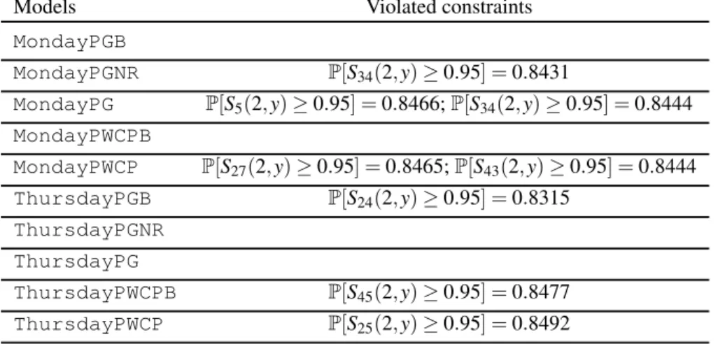
5.I Violated constraints for out-of-sample simulations of the ten models. . . 54 5.II Mean and standard deviation of the staffing costs with the sample size 1000. 60 5.III The violated constraints for the out-of-sample simulation of the ten models

with low occupancy. . . 63 5.IV The constraints which are not satisfied for the out-of-sample simulation of

LIST OF FIGURES

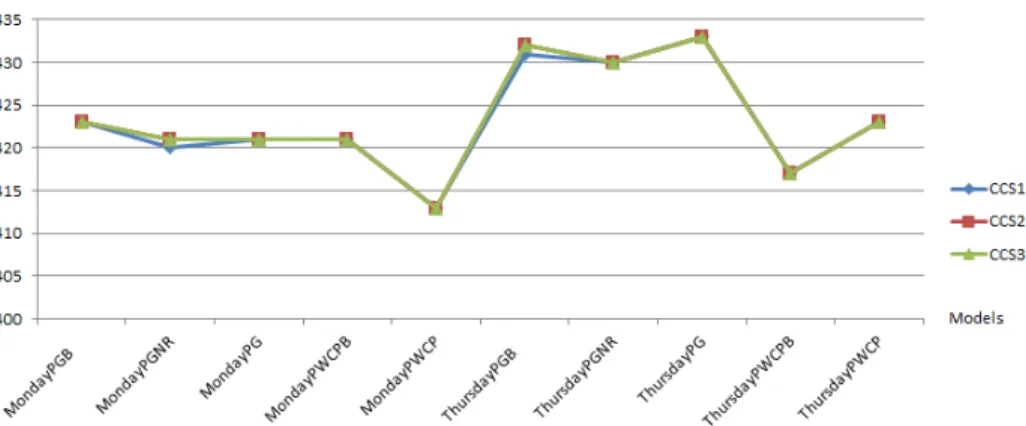
5.1 Total costs of final solutions with the three algorithms for 1000 replications. 50 5.2 Staffing levels obtained from Erlang C and algorithm CSS3 for 1000

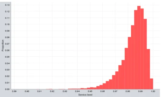
repli-cations of MondayPGB. . . 50 5.3 The distribution of the SL in the whole day of the model MondayPGNR

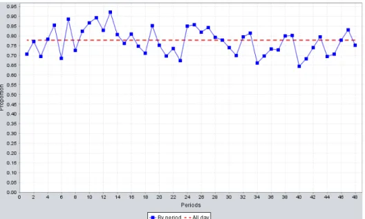
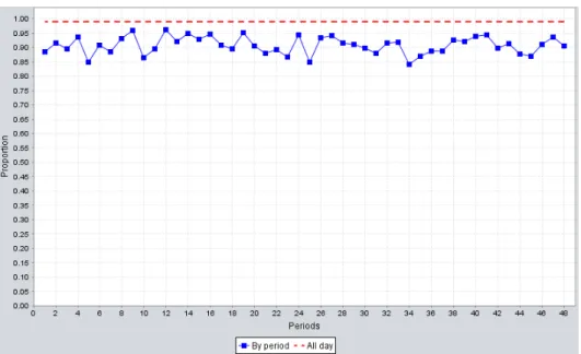
with the staffing level obtained by Erlang C. . . 51 5.4 Proportion of the days where the SL constraint is satisfied, for each period,

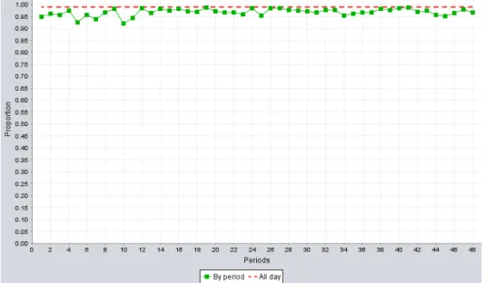
over 10000 simulated days, for the MondayPGNR model, with the staffing level obtained by Erlang C.. . . 52 5.5 Proportion of the days where the AWT constraint is satisfied, for each

pe-riod, over 10000 simulated days, for the MondayPGNR model, with the staffing level obtained by Erlang C. . . 53 5.6 The distribution of the service level in the whole day of the model MondayPGNR

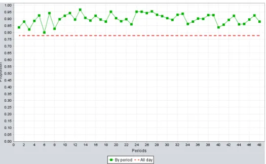
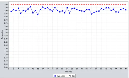
with the staffing level obtained by CCS3.. . . 55 5.7 Proportion of the days where the SL constraint is satisfied, for each period,

over 10000 simulated days, for the MondayPGNR model, with the staffing level obtained by CCS3. . . 56 5.8 Proportion of the days where the AWT constraint is satisfied, for each

pe-riod, over 10000 simulated days, for the MondayPGNR model, with the staffing level obtained by CCS3. . . 57 5.9 Proportion of the days where the SL constraint is satisfied, for each period,

over 10000 simulated days, for the MondayPGNR model, with the staffing level obtained by increasing one agent in period 34 from the staffing level obtained by CCS3. . . 58 5.10 Proportion of the days where the SL constraint was satisfied, for each

period, over 10000 simulated days, for the MondayPGBNR model, with the staffing level obtained by decreasing one agent in period 12 from the staffing level obtained by CCS3. . . 59 5.11 Staffing levels obtained by Erlang C and CCS3 of the MondayPGB∗model. 60

5.12 Proportion of the days where the SL constraint is satisfied, for each period, over 10000 simulated days, for the MondayPGB∗model with the staffing level obtained by Erlang C.. . . 61 5.13 Proportion of the days where the SL constraint is satisfied, for each period,

over 10000 simulated days, for the MondayPGB∗model with the staffing level obtained by CCS3. . . 62 5.14 Proportion of the days where the SL constraint is satisfied, over 10000

sim-ulated days, for the MondayPGNR∗model, with the staffing level obtained from CCS3. . . 64 5.15 Proportion of the days where the SL constraint is satisfied, over 10000

sim-ulated days, for the MondayPGNR∗model, with the staffing level obtained by increasing one agent in period 43 from the staffing level obtained by CCS3. . . 65 5.16 Proportion of the days where the SL constraint is satisfied, over 10000

simulated days, for the MondayPGBNR∗model, with the staffing level ob-tained by decreasing one agent in period 8 from the staffing level obob-tained by CCS3. . . 66 5.17 Staffing levels obtained by Erlang C and CCS3 of the MondayPGB∗∗model. 67 5.18 Staffing levels obtained from CCS3 before and after adding stage Correction

of MondayPGB∗∗. . . 67 5.19 Proportion of the days where the SL constraint is satisfied, over 10000

sim-ulated days, for the MondayPGB∗∗model, with the staffing level obtained by CCS3. . . 68 5.20 Proportion of the days where the SL constraint is satisfied, over 10000

sim-ulated days, for the MondayPGB∗∗model, with the staffing level obtained by decreasing one agent in period 11 from the staffing level obtained by CCS3. . . 69 5.21 Staffing levels obtained from Erlang C and algorithms for 1000

replica-tions of MondayPGB₂. . . 70 5.22 Proportion of the days where the SL constraint is satisfied, for each period,

over 10000 simulated days, for the MondayPWCP₂model, with the staffing level obtained by CCS3. . . 71

xi 5.23 The distribution of the service level in the whole day of the model MondayPWCP2

with the staffing level obtained by CCS3.. . . 71 5.24 Proportion of the days where the SL constraint is satisfied, over 10000

sim-ulated days, for the MondayPWCP2model, with the staffing level obtained

by decreasing one agent in period 46 from the staffing level obtained by CCS3. . . 72

AHT : Average Handle Time;

ASA : Average speed of answer, average waiting time of calls; AWT : Average waiting time;

CCS1 : First chance-constrained staffing algorithm; CCS2 : Second chance-constrained staffing algorithm; CCS3 : Third chance-constrained staffing algorithm;

FCFS : First come, first served, routing policy first come, first served; FIFO : First in, first out, a synonym of FCFS;

PG : Poisson-Gamma;

PGB : Poisson-Gamma with busyness factor; PGNR : Poisson-Gamma NORTA rates; PWCP : Piecewise constant Poisson;

PWCPB : Piecewise constant Poisson with busyness factor; QoS : Quality of service;

SL : Service level;

SLLN : Strong law of large number; TSF : Telephone service factor;

WFM : Workforce Management, management of labour; w.p.1 : With probability 1.

NOTATION

c Vector of size I × Q that represents the cost of each agent group in each shift;

d Vector of size I × P that represents the cost of each agent group in each period;

E(·) Expectation operator; I Number of agent groups; i∈ {1, ..., I} Agent group i;

K Number of call types; k∈ {1, ..., K} Call type k;

N Set of natural numbers; P(·) Probability operator;

P Number of periods; p∈ {1, ..., P}: Period p;

Q Number of shifts; q∈ {1, ..., Q} Shift q;

R Set of real numbers;

r Probabilities which the service level constraints are satisfied; s Service level target;

Si All types of calls that can be served by agents in group i;

v Probabilities which the average waiting time constraints are satisfied; w Acceptable waiting time in the average waiting time constraints;

x Vector of size I × Q representing the number of agents in each group in each shift;

y Staffing vector of size I × P that represents the number of agents in each group at each period;

τ Acceptable waiting times in the service level constraints; λ Call arrival rate.

I would like to express my gratitude to my supervisor Pierre L’Ecuyer for his support, for the useful comments, remarks and his engagement through the learning process of this master thesis. He has always helped me to see a clearer and bigger picture, listened carefully to my ideas and analysed my idea by the best of his knowledge and belief. I am honoured to be working with such an experienced and intelligent professor. Furthermore, I would like to thank my co-supervisor Fabian Bastin for his valuable comments both in my work and in this thesis, for many interesting discussions. Indeed, he is always enthusiastic whenever I need his help.

I thank my colleges in Simulation and Optimization Lab: Richard Simard, Wyean Chan and Nazim Regnard for the stimulating discussions, for their useful experience as I started my research, and for all the fun we have had in the last two years.

I am grateful to my professor Michel Toulouse, who introduced me to my professors Pierre L’Ecuyer and Fabian Bastin, and gave me lots of valuable advices.

Also, I would like to thank my best friend, Tien Mai Anh, who is also my college in my lab. He always encouraged me whenever I met difficulties. Therefore, I am always confident with all his support. I will be grateful forever for his love.

I also want to thank all my Vietnamese friends in Montreal, for their help at the first time I came to this beautiful city, for their valuable experience about the new life and new research environment in Canada. I am grateful to my professors in Department of Computer Science and Operations Research, who gave me precious lessons and paved the way for the completion. I also truly appreciate the excellent service provided by the departmental administrators and departmental secretaries. The list is long so I do not enumerate them here.

Finally, I would like to dedicate this thesis and all of my academic achievements to my parents, my sister and all the people in my family who have been anxiously waiting for its completion.

CHAPTER 1

INTRODUCTION

Telephone call centers are key components of many businesses, and their economic role is growing. They are used to handle customer support, phone orders and sales, marketing, governmental information services (police, ambulances,...), etc. Call cen-ters have become a popular means for companies to communicate with their customers. Some call centers are very essential and it would be really difficult to imagine a govern-ment agency, financial institution or 911 emergency services without telephone service. The call center industry is thus large and rapidly expanding, in terms of both work-force and economic scope. It employs millions of people around the world and is fast growing. In the United States, according to statistics from the Bureau of Labor Statistics [11], agents in customer service rank 7th in the list of the largest occupations in 2010. This agency estimates that there were approximately 2.3 million agents in the U.S. in 2008 with 23% working in the financial and insurance sectors and 15% in the area of administration and support service (Bureau of Labor Statistics [8]). Most of these em-ployees work in call centers, but the data also contains agents who interact directly to clients. The research predicts an increase in the number of jobs by 18% to 2.7 million in 2018. Another report estimated that there were 2.15 million agents in May 2010 with average hourly wages of US $15.76 and median of US $14.64 and an average annual salary of US $32780 (Bureau of Labor Statistics [10]). The annual salary cost of agents is then estimated at US $70.3 billion in 2010 in the United States. For comparison, in May 2007 (before the financial crisis of 2008-09), there were 2.2 million agents and an average annual salary of US $31040 for a total labor cost of US $68.1 billion (Bureau of Labor Statistics [9]). Because call centers typically spend 60% to 70% of their budgets on labor costs (Gans et al. [16]), it is important to optimize the management of labor. Their management is complex and is a major area of application for operations research.

1.1 Description of call centers

Gans et al. [16] and Koole [22] provide a good description of the functioning of a call center and the different stages that a call must pass before being answered by an agent. A call (or contact) represents a communication between a client and a service. A call is also distinguished by its issuer: it can be emitted by a client (incoming call) or by an agent (outgoing call). These calls are generally classify by type, representing the requested service and its source of origin. An employee who interacts with the customer on the phone is called an agent or representative customer service. Agents sharing a common set of tasks form a group of agents. Each of them requires special skills on the part of the employees: language, technical knowledge of a specific product, etc. A group of agents is called specialist if it is assigned to some tasks and general in the case of multiple tasks. When the skill-level required to handle calls is low, each employee is trained to handle every type of call, and calls may be handled first come, first served (FCFS), also called first in, first out (FIFO). Otherwise, if more highly-skilled works are required, each agent may be trained to handle only a subset of the types of calls, a “skills based routing”may be used to route calls to appropriate agents. Obviously, a client can be transferred through several staffs before being satisfied. There are various kinds of call centers: inbound call centers service ingoing calls, outbound call centers handle outgoing calls, a call center that handles these mixed operations is referred to blend incoming and outgoing center. In our context, we only consider inbound call centers. A staff is called multi-purpose when an agent can serve several types of calls. Besides the cost of training, the cost of an agent is often determined by the number of tasks assigned to the group.

1.1.1 Inbound call handling

Customers call the centers for various reasons. When a call arrives, a free agent is selected among agent groups. The router uses the type of the call to determine which agents are allowed to serve the call, and how agents are chosen if several agents are free. If a free agent is found, the call is sent to that agent, and the agent is allocated for a

3 certain service time. If no agent is available for a new call, the call is sent to a waiting queue if that does not exceed the total queue capacity. A call entering queue balks if it abandons immediately. Other calls having to wait join the queue where they remain until agents are free to serve them. A queued caller can also become impatient, and abandon without service. If the queue is full at the time of an arrival call, the call is blocked instead of entering the queue, i.e., the caller receives a busy signal.

1.1.2 Performance measures

Performance measures allow to assess the quality of service and efficiency of a call center. The main purpose of these performance measures is to ensure the call center is meeting its goals and objectives. Among them, service level (SL) is one of the most pop-ular. It denotes the percentage of calls that are answered in a defined waiting threshold. The constraint on the SL is most commonly stated as s percent of calls answered in τ seconds or less, where τ is a parameter, and is usually denoted by s/τ. The SL can be measured and controlled separately by time period (hour, day, etc.) and by call type, or in an aggregated way. Many contact center managers simply assume that a target of 80/20 is the industry standard, and therefore use that as their own target. While this may be the most common service level for customer service call centers, the fact is that there is no industry standard for the SL. Other centers such as 911 in Montreal or emergency set their standards to 95/2. Similarly technical support centers often have as target service level waiting times of 3 to 5 minutes for free support (Seyrafiaan [32]). In practice, call centers set their overall target (both percentage of calls and the threshold) in conjunction with their Work Force Management (WFM) division in order to calculate their staff re-quirements and scheduling. A higher service level means faster service (answering the call) for customers. An important motivation for studying this measure is that for many types of call centers that provide services, in several countries, there are government reg-ulations on the minimal acceptable SL and the call centers may have to pay very large fines when this SL is not met. As we will see in Section 2.2, over a given time period, the SL is a random variable. Therefore, from the optimization point of view, ensuring the target over finite durations can be expressed by chance constraints. One may prefer

to define the SL over a long-term (infinite-horizon) in order to work with expectations only, but this only ensures that the target is met on average.

The definition of SL also encourages us to give priority to calls who waited less than or equal to τ, because serving those who waited more than τ can not improve the measurement. In other words, while the SL indicates the percentage of calls that were answered within the waited threshold, it does not provide any information regarding the remaining calls. For this reason, it is important to look at a measure that represents all the callers, such as the average waiting time (AWT) or average speed of answer (ASA). The AWT or ASA in a period is the average (or mean) time a customer waited to have a service for this period. For example, in a time interval, if half the calls go into queue and wait for an average of 30 seconds, and the other calls go immediately to an agent, the average waiting time is 15 seconds. Obviously, a lower service level (lower percentage of calls or longer threshold) produces a longer ASA. Combined with the SL, the ASA provides a more complete picture of the flow of the incoming calls. Another measure is the abandonment ratio, which is measured by looking at the calls that abandon during the defined time period compared with all calls for that period. Service level and average waiting time are two quality of service (QoS) measures.

The satisfaction and well-being of agents influence the performance of a call center. A manager often measures the efficient use of call center agents by the occupancy ratio of agents. It is the percentage of time an agent is busy on a call or doing after call work compared with available time. It is calculated by dividing time spent to answer calls by total time at the workplace. For a call center with a high volume of calls and a lot of agents, it is often possible to have a high quality of service with an occupancy rate of over 90%. If occupancy is too low, agents are idle. If occupancy is too high, agents are overworked, so they will be less effective, because the agents are exhausted. The art of the workforce management (WFM) process is to create a balance between the SL and the occupancy ratio. Practice shows that for most (though not all) centers, an occupancy ratio of between 75% to 85% is optimal. However, not every call center or agent group can reach that number. Small call centers that wish to deliver an 80/20 service level and have sufficient staffing in place may not be able to achieve occupancies above 70% or

5 80%. Larger call centers have the opposite problem. Their large group efficiencies may allow them to staff for the same 80/20 service level and have occupancy numbers over 95%. In such cases, these managers have to add extra workers to bring occupancy down to a tolerable level (Reynolds [31]). Many other different performance measurements used to gauge the efficiency and effectiveness of a call center operation are discussed in Reynolds [31].

1.1.3 Workforce Management

Workforce management is an essential part of the operation in any call center. It can be summed up as a series of activities related to forecasting call volumes, and scheduling required and appropriate staff. A complete WFM process is required to create planning documents, call volume forecasts, agents schedules and intra-day adjustments (Seyrafi-aan [33]).

Planning As the name implies, the planning stage is where it all begins. Using high level forecasting techniques, call centers can come up with their expected annual work-load (work-load is the total time required to handle the arrival calls). From here, the centers can calculate the overall staffing requirements, hiring timelines, training requirements and timelines as well as vacation allocation and the total budget.

Forecasting A typical forecast predicts call volumes for any given time intervals in a day (majority of centers use 15 or 30 minutes intervals) for the forecasting period. Forecasting stage is based on the historical call patterns. However, there may be some requirements for final adjustments based on the latest information as well as changes in the environment.

Scheduling After forecasting the number of incoming calls for each interval, the next step is to determine the number of agents required for each interval. But WFM is more than simply determining agents for a day. Managers also schedule lunches, breaks, scheduled trainings and vacations, and deal with the 2-3% of staff that will not show up for their shift.

Intra-day adjustments Even with the best laid plans and calculations, it is necessary to track the operation of the queue (call volumes, service level) and adjust the staffing to ensure that the center is providing the best service level possible, while maintaining a reasonable occupancy rate. An intra-day adjustment team is re-sponsible for tracking and reporting the operational indicators, re-forecasting the daily volumes (usually twice a day), reassigning staff to and from various off-line activities and maintaining the overall target service level.

1.1.4 Description of emergency call centers

Our work focuses on emergency call centers. Emergency services call centers are a specialised component of the call center industry. An emergency is any situation where the safety of people or property is at risk and requires immediate assistance. For exam-ple, 911 is the emergency telephone number for the North American Numbering Plan. This number is intended for use in emergency circumstances only, and to use it for any other purpose (including non-emergency situations and prank calls) can be a crime. Ex-amples of the 911 emergencies in Canada include: a fire, a crime in progress or a medical emergency. A general view of an emergency call center is a call center where agents are trained to answer calls from emergency situations. In the context of an inbound emer-gency services call center, the organisation has no control over the arrival rate which depends on natural and human phenomena (Lewis et al. [29]). Although many calls do arrive randomly, some kinds of incidents generate spurts of calls that are related to the same incident and so are not truly random. For example, a visible fire will usually gener-ate many calls from the area. Calls will peak within several minutes and then downgrade as the fire suppression units arrive. Most of the calls within a short period will be related to the same incident, together with random calls also arriving interspersed among the fire calls. Many other kinds of incidents also generate multiple calls, creating a large spurt of call arrivals, and such effects demand more personnel to handle them. However, it is not uncommon to see overlapping spurts, which further stresses the emergency systems. Nobody knows in advance when such bursts can happen, so one cannot put more per-sonnel at the right time. What is possible is to put one or a few more agents most of the

7 time to cover this possibility. According to Lewis and Herbert [28], the emergency call centers provide support to the community by a high level of service when needed. Their effectiveness is gained by operation through efficient scheduling, rapid response to calls and a high standard of agent capability. Therefore, the service level should be very high and average waiting times are very low. Lafond [23] shows an example where 90% of all 911 calls arriving shall be answered within 10 seconds during the busy hour (the hour each day with the greatest call volume) and 95% of all 911 calls should be answered within 20 seconds. The 911 center in Montreal requires that 95% of all arriving calls shall be answered within 2 seconds. The requirements of high service levels and low average waiting times in emergency call centers imply that the occupancy of agents will be low.

1.2 Literature review

First, we give some definitions of Staffing, Scheduling and Routing Problems of call centers. The goal of these problems is to minimize the operating cost of the center under a set of constraints on certain performance measures such as SL, AWT and so on. One decision to be made is how many agents of each skill group to have in the center as a function of time. In a staffing problem, the day is divided into periods (e.g., 30 minutes or one hour each) and one simply decides the number of agents of each group for each period. In a scheduling problem, a set of admissible work schedules is first specified, and the decision variables are the number of agents of each skill group in each work schedule. This determines the staffing indirectly, while making sure that it corresponds to a feasible set of work schedules. A yet more restrictive version of the problem is when there is a fixed set of available agents to be scheduled for the day or the week, where each agent has a specific set of skills. Then we have a scheduling and rostering problem. In this thesis, we focus on the staffing problem for inbound call centers. This section provides a survey of the recent literatures and various tools which can help solve this problem.

1.2.1 Modeling a call center

Modelling a call center is difficult because it is common to have only the averages of performance measures over each period of the day, e.g., a half hour. It is difficult to find the appropriate distributions and dependencies between random variables with such aggregated data.

The arrival process of calls is not a homogeneous Poisson process (deterministic rate). However, we often make this assumption, for the sake of mathematical simplicity. More recent studies suggest a double stochastic process, e.g., Poisson-Gamma, if the arrival rate of the Poisson process is a random variable (Avramidis et al. [2], Brown et al. [6], Jongbloed and Koole [19]). Arrival rates often vary depending on the time-of-day and often on the time-of-day-of-week. A positive correlation between periods and between days was also observed in several analyses. In this thesis, we consider several arrival processes which are discussed in Oreshkin et al. [30]. We give more details to explain these arrival processes in Section 5.1.

The service time of a call is often regarded as a random variable following an expo-nential distribution. Brown et al. [6] suggests that the lognormal distribution is usually a much better fit.

Several other processes are less studied; data are often unavailable or partially con-ditional on certain events. The patience time determines the time a customer is willing to wait before giving up. It is important to model the patience time distribution correctly because it can have a significant effect on the SL and abandonment ratio. Estimating the patience distribution requires special statistical techniques (Brown et al. [6]).

1.2.2 Simulation tools

Simulation is a very flexible tool which generally requires less advanced knowledge of mathematics that the analytical models. The widening gap between the evolution of actual call centers and the development of analytical models is one of the main reasons for the popularity and the need of simulation tools. However, simulation is a complex program that requires considerable development effort. Based on the collection of

statis-9 tics, simulation requires significant lead time to reduce the noise and the confidence interval of the measurements.

For the optimization software discussed in our thesis, we use a simulator built from a Java library for simulating contact centers (Buist and L’Ecuyer [7]), see also http:// www.iro.umontreal.ca/˜simardr/contactcenters/index.html. It is based on the well-supported modern programming language Java and is built over the SSJ simulation library (L’Ecuyer [25], L’Ecuyer and Buist [26]).

1.2.3 Call center staffing problem

The call center staffing problem has received a great deal of attention in the literature. Staffing in the single-skill case (i.e., single call type and single agent type) has received much attention in the call center literature. It is common to divide the day into several periods during which the staffing is held constant and the arrival rate does not vary much. The system is often assumed to reach steady-state, and steady-state queueing models are used to provide a staffing for each period. The simplest queueing model of a call center is the M/M/n queue, also known as an Erlang C system. This model ignores blocking and customer abandonments. We will discuss this system in more detail in Section 2.1. However, this assumption never happens in the real call centers, so it is a crude approximation made in each time period. For better accuracy, the staffing and scheduling should be done using simulation, as in the following articles.

Atlason et al. [1] propose a general methodology, based on the cutting plane method of Kelley [21], to optimize the staffing of agents in a call center with single call type and single skill, under service level constraints. They formulate the constraints in terms of infinite horizon service levels. Their method combines simulation with integer pro-gramming and cut generation. First, they relax the staffing problem to a sample average approximation(which becomes a deterministic problem). Then, they optimize this sam-ple problem by generating cuts from the violated service level constraints and adding corresponding linear constraints. This process terminates when the optimal solution of the relaxed problem is feasible for the original problem.

a single period in steady-state is already difficult; the Erlang formulas and their approx-imations (for the SL) no longer apply. Simulation seems to be the only reliable tool to estimate the SL. Cez¸ik and L’Ecuyer [12] extend the method of Atlason et al. [1] to the multiskill call centers. They also show some difficulties encountered with larger problems, and develop (heuristic) methods to deal with these problems.

In order to solve the multiskill scheduling problem, Bhulai et al. [5] propose a two-step approach. The first two-step determines a staffing of each agent type for each period. In the second step, it solves a linear program to find a set of shifts that cover this staffing by allowing agents to use only a subset of their skills in certain periods if needed. Bhulai et al. [5] recognize that their two-step approach is generally suboptimal and they illus-trate this by examples.

Avramidis et al. [3] propose a simulation-based algorithm for solving the multi-skill scheduling problem, and compare it to the approach of Bhulai et al. [5]. This algorithm extends the method of Cez¸ik and L’Ecuyer [12], which solves a single period staffing problem.

In typical problem formulations, the constraints with respect to the average perfor-mance measures in the long run are considered. Gurvich et al. [17] propose a more ap-propriate problem formulation, which is to use probabilistic constraints on the (random) values over a given time period. The form is as following: the call center’s management chooses a risk level δ , and allows the QoS to be violated on at most a fraction δ . They consider the probabilistic constraints on the abandonment ratios, with random (but time-independent) arrival rates, and use a fluid approximation of the abandonment ratios for any realization of the arrival rate. Moreover, they develop a two-step method to optimize the staffing (for the staffing problem) under chance constraints. The first step introduces a Random Static Planning Problem (RSPP) and discusses how it can be solved using two different methods. The RSPP finds a set of staffing levels that minimize staffing costs subject to the requirement that the staffing levels are sufficient to meet the demand of all types of calls with a probability that is 1 − δ . The output of the RSPP is a staffing solution and a set of arrival rate vectors which are called the staffing frontier. In the second step, they solve a finite number of staffing problems with known arrival rates –

11 the arrival rates on the optimal staffing frontier. Thus, the most important role of the staffing frontier approach is that it reduces the complex staffing problem with uncertain rates to one of solving multiple problems with predictable rates. In the end, the output is a staffing and routing solution that is feasible to chance constraints and is nearly optimal for large call centers.

1.3 Master’s project

The management of labour in call centers is a difficult optimization problem. There are lots of studies in this field. Some formulas as well as few algorithms to solve the staffing problem in call centers have been proposed in literature. As discussed above, the authors formulate the constraints in long term average performance measures over an infinite horizon. This type of formulation stems from historical reasons, but it is not necessarily appropriate for some practical applications. Even if the average is satisfied the target threshold, the service level on a given day is a random variable that may have a large variance, and may take a value much smaller than the target for a significant fraction of the days. Therefore, according to the suggestion of Gurvich et al. [17], in this thesis, we consider the use of probabilistic constraints expressing that the service level targets (per call type, per period, global) on a random day must be satisfied with probability at least 1 − δ , for a given risk level δ selected by the manager. We are also interested in constraints on the average waiting time. The goal is to design an optimiza-tion software to find the optimal allocaoptimiza-tion while satisfying these constraints, therefore defining a simulation-based optimization problem. We adopt the “sample-average ap-proximation”approach for solving this problem, as described in the following. First, we generate the simulation input data for N independent replications of the operations of the call center over the planning horizon. This data includes call arrival times, service times and so forth. When this data is fixed, we can estimate the probabilities in the constraints by the averages computed over the generated realizations. Then, we solve a determinis-tic optimization problem that chooses staffing levels so as to minimize the staffing cost, while ensuring that the constraints are satisfied. Then, we study the convergence of the

optimal solution of the sample problem to that of the original problem. By using the strong law of large numbers (SLLN), we show that the set of optimal solutions of the sample problem is a subset of the set of optimal solutions for the original problem with probability 1 (w.p.1) as the sample size gets large. Furthermore, we show that the prob-ability of this event approaches 1 exponentially fast when we increase the sample size. We do all of these in a multiskill setting. In this thesis, we focus our attention on solving the sample-average approximation problem for the single agent type call centers, and propose three simulation-based optimization algorithms. The original idea is to increase the staffing in periods where the constraints are violated, and to decrease the number of agents in each period as much as possible while still satisfying the requirements. We prove that these methods terminate under some conditions and analyse the quality of the solutions obtained by the algorithms. We also include extensive numerical experiments in several different types of call centers to assess the performance of these algorithms.

1.4 Structure of the thesis

This thesis is divided into six chapters. Chapter 1 presents the overview about call centers and some related problems. In Chapter 2, we model the staffing problem by using chance constraints with respect to the service level and the average waiting time. In Chapter 3, we define the sample average approximations of the chance-constrained staffing problem in the multiskill setting. This chapter also considers the convergence of optimal solutions of the sample problem to the real optimal staffing level in the original problem. In Chapter 4, we propose three simulation-based optimization algorithms to solve the sample average approximations for the special case where all agents have all skills (a single group of agents). Chapter 5 measures the efficiency of each algorithm in several instances. We use the real data from an emergency call center 911 which has low occupancy. We also test the algorithms in other call centers which have much higher occupancy. Then, we consider the heavy traffic call center models to assess the quality of our algorithms.

CHAPTER 2

MODEL AND PROBLEM FORMULATION

This chapter introduces the main problem of this thesis in mathematical form. This problem is the management of the workforce for a number of specific groups assuming an infinite number of available agents per group. We define the scheduling problem in a multiskill setting in this section.

2.1 Erlang C traffic model on call centers

In this section, we give some definitions for the Erlang C traffic model for a single call type. According to Cooper [14], a queuing model can be defined in terms of three characteristics: the input process, the service mechanism, and the queue discipline. The queuing models which we consider in this section are built under the following assump-tions: the customers are assumed to arrive according to a Poisson process with constant rate λ , the service times are assumed to be exponentially distributed with rate µ and independent of each other (as well as everything else in the system); the queue disci-pline is assumed to be blocked customers delay, i.e., when blocked customers wait as long as necessary for service; the waiting calls are handled FIFO; and there are n agents. These queuing models are called the M/M/n queue. The number of waiting positions in the queue is assumed to be infinite. The offered traffic load is defined by ρ = λ

µ. Let

C(n, ρ) denote the probability that all servers are occupied. According to Cooper [14], the formula to compute C(n, ρ) is:

C(n, ρ) = ρn n!(1−ρ/n) ∑n−1_k=0ρ k k! + ρn n!(1−ρ/n) , (0 ≤ ρ < n). (2.1)

This is called the Erlang delay formula or Erlang C formula. The Erlang C formula was first published by by A.K. Erlang in 1917. Since an arriving call has to wait if all servers are busy, the delay probability P[W > 0], where W is the waiting time of a call,

is given by (2.1). The SL for a given n is computed from

P[W ≤ τ ] = 1 − C(n, ρ )eτ (nµ −λ )with τ ≥ 0. where τ is the acceptable waiting time.

The Erlang C function computes the probability that an arrival call in the Erlang C queueing model will find all servers busy. This is the same as the fraction of arrival calls that are delayed (i.e., must wait) before being answered. The service level estimate given by the Erlang C formula is the average over an infinite time horizon. The Erlang C formula describes the relationship between the call-arrival rate, the average service time, the service level, and the number of agents. If we know any three of these numbers, we can calculate the unknown factor. Generally, we are calculating the staff number needed to achieve a service level or we are calculating the expected performance (service level) of a number of staffings. The minimum n required to meet a given target of SL s, i.e., minn≥0{n : P{W ≤ τ} ≥ s}, can be obtained by some methods, using the fact that the

SL is monotone in n. In our thesis, we use the Erlang C formula and the binary search to find the required number of staffs.

However, when n is very large and the system has high utilization, using the exact Erlang C formula is quite difficult. Halfin and Whitt [18] give an approximation to the Erlang C in this case. They consider a sequence of M/M/n queues for which n → ∞ and (1 − γ)√n→ β for 0 < β < 1, where µ is fixed and γ = λ /(nµ) is the associated average system utilization or occupancy (also called “traffic intensity”). And they prove that

P[W > 0] −→ 1

1 + β Φ(β )/φ (β )

where Φ and φ are the standard normal distribution function and density, respectively. They show that when the offered load ρ is high, and an appropriate number of agents are employed, a system can achieve a high agent utilization and yet deliver a good service level by choosing the number of servers as n = ρ + β√ρ + o(√ρ ). If omitting the small order term, we call this square-root safety staffing. If γ is fixed while λ and µ increase to infinity, then P[W > 0] converges to 0, i.e., nobody waits in the limit. This is

15 called the quality-driven regime. It is appropriate for situations where speed of answer is much more important than the cost of agents, e.g., emergency service. In another case, if the safety staffing β√ρ is fixed while both λ and n increase to infinity, then P[W > 0] converges to 1, so in the limit, everyone waits. This efficiency-driven regime is appropriate for call centers where the productivity of agents is much more important than the wait, i.e., an answering email system. Another regime called a quality and efficiency-driven(QED), is a regime for which P[W > 0] is fixed to a constant in (0, 1) while λ and n increase to infinity. It is good for a large call center with constraints on the SL and abandonment ratio.

2.2 Performance measure

We describe in more details the performance measures introduced in Section 1.1.2. In reality, the performance measures are calculated from the observed data at the end of a period or day. There is no unique formula or standard for measuring performance. There are often many different formulations to compute these measures. In many opti-mization problems studied so far, a general approach is to consider the expected perfor-mance measures over an infinite time horizon. However, in this context, we would like to consider the distributions of performance measures in a given time interval, not the expected value. We present in this section the performance measures used in this thesis or considered important.

The service level (SL) is one of the measures which is most used in industry. This measure is also referred to as telephone service factor (TSF). The formula for the SL is not unique, but it can be summed up as the fraction of calls answered within a given time τ , where τ is a parameter which is called acceptable waiting time. We present only some formulas of service level and distinguish the definitions of service level over a given time period and in a long run. Many other formulas are proposed in Jouini et al. [20]. Let S(τ,t1,t2) be the number of calls served after a waiting time less than or equal to τ during

interval [t1,t2]. Let N(t1,t2) be the total number of calls counted during interval [t1,t2]

or equal to τ during the same time interval. Since the arrival and service times of calls are not known but are random, the service level in a given time period [t1,t2] will be a

random variable and a formula of service level in the time interval [t1,t2] is

f_S1(τ,t1,t2) =

S(τ,t1,t2)

N(t1,t2) − L(τ,t1,t2)

. (2.2)

This definition of service level (2.2) is used in our formulation with chance constraints. For any given fixed staffing of agents, no reliable formula or quick algorithm is available to estimate the distribution of service level; it can be estimated with a long (stochastic) simulation only. An example of chance-constraint on the service level is, for example, the probability that at least 95% of calls are answered within τ = 2 seconds in a given time period is equal to or greater than 85%. This constraint is used for the model of the emergency call center 911 in Montreal in our numerical experiment.

Another formula of service level defines the long-term fraction of calls whose time in queue is no larger than a given threshold, that is:

f_S2(τ,t1,t2) = E[S(τ , t1

,t2)]

E[N(t1,t2) − L(τ,t1,t2)]

, (2.3)

where E denotes the mathematical expectation.

In this definition, the numerator is the average of calls answered within τ and the denominator is the average number of arrival calls (without abandonments), over an infinite time horizon. The service level defined in (2.3) is equal to the fraction of calls answered within τ over an infinite number of independent and identically distributed (i.i.d.) copies of intervals [t1,t2]. It was used in most previous articles on staffing and

scheduling optimization (e.g., Atlason et al. [1], Avramidis et al. [3], Avramidis et al. [4], etc). Multiple measures of SL are of interest: for a given time period of a day, for a given call type, for a given combination of call type and period, aggregated over the whole day and all call types, and so on. A typical constraint on the SL is, for example, that 80% of calls are answered within τ = 20 seconds. In these contexts, they approximate f_S2by simulations, the expectations being estimated by the sample averages.

17 also can distinguish two situations: the expected value over an infinite time horizon or the random variable in a given time period. We here focus on the service level calculated in a given time period; the extension to infinite horizon is direct. The first alternative considers abandoned calls who waited less than or equal to τ as “good served calls”:

f_S3(τ,t1,t2) =

S(τ,t1,t2) + L(τ,t1,t2)

N(t1,t2)

. (2.4)

Another alternative formula considers all abandonments as “badly served calls”:

f_S4(τ,t1,t2) =

S(τ,t1,t2)

N(t1,t2)

. (2.5)

Another performance measure is the average waiting time. It is the average (or mean) length of time a customer waited to have a service. The average waiting time is calcu-lated by diving the total number of waiting time of all calls, by the total number of calls during the time period. Similar to the service level, we also have many definitions of av-erage waiting time. We give two formulas for this measure, the former being computed over a given time period and the latter being defined for a long run.

A formula of average waiting time over a given time period [t1,t2] is:

f_W1(t₁,t₂) =W(t1,t2) N(t1,t2)

, (2.6)

where W (t1,t2) is the sum of waiting times of calls (served or abandoned) counted during

time interval [t1,t2]. The average waiting time in this definition is a random variable, and

is used in our formulations with chance constraints. An example of the chance constraint with average waiting time is that the probability that the average waiting time in a given time period does not exceed 2 seconds is no smaller than 85%.

An alternative definition represents the average waiting time within a given time [t1,t2] in the long run:

f_W2(t1,t2) = E[W (t1

,t2)]

E[N(t1,t2)]

. (2.7)

the average sum of waiting times by the average number of arrivals.

For other performance measures discussed in the following, we also distinguish them in two definitions, the expected value over the long run and the random variable in a given time interval. We only describe here their definitions as random variables.

An important measure is the abandonment ratio, defined as:

f_A(t1,t2) =

A(t1,t2)

N(t1,t2)

, (2.8)

where A(t1,t2) is the total number of abandonments. Abandonments usually mean the

loss of potential customers.

The effectiveness of a call center is also often measured by the occupation rates of agents. Let yi be the number of agents in the group i, T be the time horizon covered

by the measure and Gi(t) ≤ yi be the number of agents of group i occupied in the time

0 ≤ t ≤ T . The occupancy ratio is defined by the proportion of agents occupied during the period of length T :

f_O,i(T ) = 1 y_iT

Z T 0

G_i(t)dt . (2.9)

2.3 Description of the model

We consider a telephone call center where different types of calls arrive at random and different groups of agents answer these calls. The calls arrive according to arbitrary stochastic processes that could be non-stationary, and perhaps doubly stochastic (see, e.g., Avramidis et al. [2]). Arriving calls that find all servers occupied line up in an infinite buffer queue. Arrivals are served in a FCFS order.

The goal is to minimize the operating cost of the center under a set of constraints on the QoS. The day is divided into periods (e.g., 30 minutes or one hour each). The objective function is the sum of costs of all agents, where the cost of an agent is a deterministic function of its set of skills.

In this context, we are interested in chance constraints on the service levels and daily average waiting times. Such constraints can be imposed per call type, per period, and globally, with different thresholds. The convergence of our sample problem and our

19 algorithms can be applied similarly when adding more constraints on other types of performance measures, e.g., abandonment ratio, occupancy ratio, etc.

Our model of a call center is composed of a set of K call types, labelled from 1 to K, and I agent types, labelled from 1 to I. Agent type i has the skill set Si⊆ {1, ..., K}. The

day is divided into P periods of given length, labelled from 1 to P. The staffing vector is y= (y1,1, ..., y1,P, ..., yI,1, ..., yI,P) where yi,pis the number of agents of type i available in

period p. Given y, let Sk,p(τk,p, y) be the fraction of calls of type k answered within τk,p

seconds during period p (the service level); let Sp(τp, y) be the fraction of calls answered

within τpseconds during period p, let Sk(τk, y) be the fraction of calls of type k answered

within τ_kseconds during the day; let S0(τ0, y) be the fraction of all calls answered within

τ0 seconds during the day; let Wk,p(y) be the average waiting time for calls of type k

during period p; and let Wp(y) be the average waiting time for all calls arriving in period

p; let W_k(y) be the average waiting time of calls of type k during the day; let W0(y) be

the average waiting time of all calls during the day. All of these are random variables, whose distributions depend on the entire staffing. Suppose that the constraints are of the form: the probabilities that service level and average waiting time are satisfied are no smaller than some given thresholds.

The service level constraints are of the form:

P[Sk,p(τk,p, y) ≥ sk,p] ≥ rk,p for 1 ≤ k ≤ K and 1 ≤ p ≤ P

P[Sp(τp, y) ≥ sp] ≥ rp for 1 ≤ p ≤ P

P[Sk(τk, y) ≥ sk] ≥ rk for 1 ≤ k ≤ K

P[S0(τ0, y) ≥ s0] ≥ r0;

where sk,p, sp, sk, s0are targets of service level and rk,p, rp, rk, r0are given constants in

The average waiting time constraints are of the form:

P[Wk,p(y) ≤ wk,p] ≥ vk,p for 1 ≤ k ≤ K and 1 ≤ p ≤ P

P[Wp(y) ≤ wp] ≥ vp for 1 ≤ p ≤ P

P[Wk(y) ≤ wk] ≥ vk for 1 ≤ k ≤ K

P[W0(y) ≤ w0] ≥ v0;

where wk,p, wp, wk, w0are targets of average waiting time and vk,p, vp, vk, v0are given

constants in (0, 1).

A shift is a time pattern that specifies the periods in which an agent is available to handle calls. In practice, it is defined by its start period (the period in which the agent starts working), break periods (the periods when the agent stops working, for instance, morning and afternoon coffee breaks, as well as a longer lunch break), and end period (the period when the agent finishes the workday).

Let {1, ..., Q} be the set of all admissible shifts. To simplify the exposition, we assume that this set is the same for all agent types; this assumption could easily be relaxed if needed, by introducing specific shift sets for each agent type. The admissible shifts are specified via a P×Q matrix B0whose element (p, q) is Bp,q= 1 if an agent with

shift q works in period p, and 0 otherwise. A vector x = (x1,1, ..., x1,Q, ..., xI,1, ..., xI,Q),

where xi,qis the number of agents of type i working shift q, is a schedule. The cost vector

is c = (c1,1, ..., c1,Q, ..., cI,1, ..., cI,Q), where ci,qis the cost of an agent of type i with shift

q. To any given shift vector x, there corresponds the staffing vector y = Bx, where B is a block-diagonal matrix with I identical blocks B0, if we assume that each agent of type

iworks as a type-i agent for the entire shift. We make the following natural assumption that every period is covered by at least one shift.

Assumption 2.3.1. For every period p there is at least one shift q such that Bp,q= 1.

Calculating the cost function is usually relatively straightforward. We can calculate the cost of each group in each shift, and multiply by the number of agents of corre-sponding group working in the shift to get the overall cost. The cost function is defined by:

21 f(y) = min x c t_x= I

∑

∑

It follows by Assumption 2.3.1 that (2.10) is feasible for any y. The value f (y) gives the minimum cost set of shifts that can cover the desired work requirements vector y. We make the following assumption on the cost vector.

Assumption 2.3.2. The cost vector c is positive.

According to Assumption 2.3.2, since c is positive and moreover, the entries in B are either 0 or 1, the α-level set of f ,

{y ∈ N: ∃x ≥ 0 and integer, Bx ≥ y, cTx≤ α},

is finite, for any α ∈ R. Define: h1_{k,p(y) = P[S}k,p(τk,p, y) ≥ sk,p] − rk,p for k = 1, ..., K, p = 1, ..., P h1_{0,p(y) = P[Sp}(τp, y) ≥ sp] − rp for p = 1, ..., P h1_{k,0(y) = P[Sk}(τk, y) ≥ sk] − rk for k = 1, ..., K h1_{0,0(y) = P[S}0(τ0, y) ≥ s0] − r0 and

h2_{k,p(y) = P[Wk,p}(y) ≤ wk,p] − vk,p for k = 1, ..., K, p = 1, ..., P

h2_{0,p(y) = P[W}p(y) ≤ wp] − vp for p = 1, ..., P

h2_{k,0(y) = P[Wk}(y) ≤ wk] − vk for k = 1, ..., K

h2_{0,0(y) = P[W0}(y) ≤ w0] − v0.

Let g : RIP→ R2(KP+K+P+1)_{be a function defined by:}

h2_0,0, h2_0,1, ..., h2_0,P, h_1,02 , ..., h2_1,P, ..., h2_K,0, ..., h2_K,P)

def

:= (g1, g2, ..., g2(KP+K+P+1)).

We are now ready to formulate the problem of minimizing scheduling costs subject to satisfying chance constraints in service level and average waiting time:

min y f(y) subject to: g(y) ≥ 0 y≥ 0 and integer. (P0)

Note that problem (P0) is equivalent to the scheduling problem:

min x c t_x= I

∑

∑

P[Wk,p(y) ≤ wk,p] ≥ vk,p for 1 ≤ k ≤ K and 1 ≤ p ≤ P

P[Wp(y) ≤ wp] ≥ vp for 1 ≤ p ≤ P

P[Wk(y) ≤ wk] ≥ vk for 1 ≤ k ≤ K

P[W0(y) ≤ w0] ≥ v0

x, y ≥ 0 and integer .

(P1)

The staffing problem is a relaxation of the scheduling problem where we forget about the admissibility of schedules and just assume that any staffing is admissible. The

23 staffing cost vector in this setting is d = (d1,1, ..., d1,P, ..., dI,1, ..., dI,P)t where di,p is the

cost of an agent of group i in period p. We have:

min y d t_y= I

∑

∑

P[Wk,p(y) ≤ wk,p] ≥ vk,p for 1 ≤ k ≤ K and 1 ≤ p ≤ P

P[Wp(y) ≤ wp] ≥ vp for 1 ≤ p ≤ P

P[Wk(y) ≤ wk] ≥ vk for 1 ≤ k ≤ K

P[W0(y) ≤ w0] ≥ v0

y≥ 0 and integer .

(P2)

In the special case where we consider one period at a time, we have d = (d1, ..., dI)t

where di is the cost of an agent of type i, suppose that d is positive and y = (y1, ..., yI)t

where yi is the number of agents of type i. In this context, we often assume that the

system is in steady-state over the given period (but we may also assume arbitrary initial conditions). The optimization problem then reduces to:

min y d t_y= I

∑

subject to: P[Sk(τk, y) ≥ sk] ≥ rk for 1 ≤ k ≤ K P[S0(τ0, y) ≥ s0] ≥ r0 P[Wk(y) ≤ wk] ≥ vk for 1 ≤ k ≤ K P[W0(y) ≤ w0] ≥ v0 y≥ 0 and integer . (P3)

In the case where we consider one call type, one agent group and P periods, we have d= (d1, ..., dP)t where dp is the cost of an agent in period p and y = (y1, ..., yP)t where

ypis the number of agents in period p. The optimization problem then reduces to:

min y d t_y= P

∑

The underlying model is typically so complex that an algebraic expression for g(y) can not be easily obtained. Therefore, simulation could be the only viable method for estimating g(y). In the next section we formulate an optimization problem which is an approximate of (P0) obtained by replacing the probability values by sample averages and prove statements about the convergence of solutions of this sample problem to the solutions of the original problem (P0) as the sample size increases.

CHAPTER 3

SAMPLE AVERAGE APPROXIMATION OF THE CHANCE-CONSTRAINED STAFFING PROBLEM

The probabilities that the service level and average waiting time are satisfied in a given period involved in the constraints are estimated by simulation. Suppose we simu-late the center N times, independently, over its P periods of operation. Let ω represent the source of randomness, i.e., the sequence of all independent U (0, 1) random variates that drive the successive simulation runs (regardless of their number). When simulating the call center for different values of a staffing level y, we assume that the same uniform random numbers are used for the same purpose for all values of y, for each day. This is implemented by using random number packages that provide multiple streams and substreams (L’Ecuyer [25], L’Ecuyer et al. [27]).

Suppose we perform N simulation runs to get the estimates of probabilities. We con-sider the distribution of the values of the service level and average waiting time over the individual runs. The empirical service-level of a simulation run, defined as the observed number of calls answered within the time limit divided by the total number of calls in this run, is a function of the staffing level y and of ω. We denote the empirical service level by the d-th replication by ˆSd_N,k,p(τk,p, y, ω) for call type k in period p; ˆSN,pd (τp, y, ω)

aggregated over period p; ˆS_N,kd (τk, y, ω) aggregated for all call type k; and ˆS_N,0d (τ0, y, ω)

aggregated overall. Similarly, the empirical average waiting time of a simulation run, defined as the total of waiting times of calls divided the total number of calls in this replication, is also a function of y and of ω. We denote the empirical average waiting time by the d-th replication by ˆW_N,k,pd (τk,p, y, ω) for call type k in period p; ˆW_N,pd (τp, y, ω)

aggregated over period p; ˆW_N,kd (τk, y, ω) aggregated for all call type k; and ˆWN,0d (τ0, y, ω)

aggregated overall. To compute these functions at different values of y, we simply use simulation with common random numbers, i.e., make sure that the same random num-bers are used at the same place for all values of y (Law [24], Chapter 10). For simplicity of notations, we omit ω from the notations.

Let h1_k,p(y; N) =∑ N d=1I[ ˆSN,k,pd (τk,p, y) ≥ sk,p] N − rk,p for k = 1, ..., K, p = 1, ..., P; h1_0,p(y; N) =∑ N d=1I[ ˆSN,pd (τp, y) ≥ sp] N − rp for p = 1, ..., P; h1_k,0(y; N) =∑ N d=1I[ ˆSN,kd (τk, y) ≥ sk] N − rk for k = 1, ..., K; h1_0,0(y; N) =∑ N d=1I[ ˆSN,0d (τ0, y) ≥ s0] N − r0; and h2_k,p(y; N) = ∑ N d=1I[ ˆWN,k,pd (y) ≤ wk,p] N − vk,p for k = 1, ..., K, p = 1, ..., P; h2_0,p(y; N) = ∑ N d=1I[ ˆWN,pd (y) ≤ wp] N − vp for p = 1, ..., P; h2_k,0(y; N) = ∑ N d=1I[ ˆWN,kd (y) ≤ wk] N − vk for k = 1, ..., K; h2_0,0(y; N) = ∑ N d=1I[ ˆWN,0d (y) ≤ w0] N − v0;

where I is the indicator function:

I[A] =     

1 if the clause A is true, 0 otherwise.

Let g : RIP× N → R2(KP+K+P+1) _{be the function of (y, N):}

g= (h1_0,0, h1_0,1, ..., h1_0,P, h1_1,0, ..., h1_1,P, ..., h1_K,0, ..., h1_K,P,

h2_0,0, h2_0,1, ..., h2_0,P, h_1,02 , ..., h2_1,P, ..., h2_K,0, ..., h2_K,P).

def

:= (g₁, g₂, ..., g_2(KP+K+P+1)).

sam-27 ple problem, and we use these notations to formulate the Sample Average Approximation (SAA) problem: min y f(y) subject to: g(y; N) ≥ 0 y≥ 0 and integer. (S1)

A similar formulation can be given for the other problems, replacing the probabil-ities on the left sides of the constrains by the sample means everywhere. The chance-constrained staffing problem for one call type, one skill agent, over a time interval di-vided into periods becomes:

min y d t_y= P

∑

3.1 Almost Sure Convergence of Optimal Solutions of the Sample Average Ap-proximation Problem

We insist on the fact that when ω is fixed, these sample problems are purely de-terministic. These are the problems we solve, instead of the original problems (P0) to (S1).

We will study the convergence of the optimal solution of the sample problem to that of the original problem as N → ∞, under the assumption that ω is really an infinite se-quence of i.i.d. random variables. Some notations as well as the process of our proof

are similar with the proof in Section 4 in Atlason et al. [1] with some variations. In that section, they prove the convergence of solutions of the sample average approxi-mation to solutions of the original staffing problem. However, the constraints in their original problem are not chance constraints, they are in terms of infinite horizon ser-vice levels. Therefore, we have some modifications to adopt for our chance-constrained staffing problem. We are interested in the properties of the optimal solutions of (S1) as the sample size N gets large. As in Atlason et al. [1], we use the Strong Law of Large Numbers (SLLN) to turn out that any optimal solution of (P0) that satisfies g(y) > 0, i.e., gj(y) > 0 for all 1 ≤ j ≤ 2(KP + K + P + 1), is an optimal solution of (S1) with

probability 1 (w.p.1) as N goes to infinity.

We say that the property A(N) holds for all N large enough w.p.1 if and only if P[∃N0< ∞ : A(N) holds ∀N ≥ N0] = 1.

The SLLN states that the sample average converges almost surely to the expected value:

X_n=X1+ ... + Xn n

a.s

→ µ for n → ∞

where X1, X2, ... is an infinite sequence of i.i.d. random variables with expected value

E[X1] = E[X2] = ... = µ and E[|Xj|] < ∞ for j = 1, 2, ....

That is, P[limn→∞Xn= µ] = 1.

We introduce some additional notations as in Atlason et al. [1]. Let g(y; ∞) := lim

N→∞g(y; N),

F∗:= the optimal value of (P0) and define the sets

Y∗:= the set of optimal solutions to (P0), Y₀∗:= {y ∈ Y∗: g(y) > 0},

Y_{1:= {y ∈ Z}IP₊ : f (y) ≤ F∗, g(y) 6≥ 0}, Y_N∗:= the set of optimal solution of (S1).

29 Note that Y1is the set of solutions to (P0) that have the same or lower cost than an optimal

solution, and satisfy all constraints except the probability constraints. We are concerned with solutions in this set since they could be feasible (optimal) for the sample problem (S1) if the difference between the sample average g(.; N) and g is sufficiently large. We show that when Y₀∗is not empty, Y₀∗⊆ Y_N∗⊆ Y∗for all N large enough, w.p.1.

The sets Y∗, Y_N∗and Y₀∗are finite by Assumption 2.3.2. (The sets Y∗, Y_N∗and Y₀∗can be empty). Furthermore, if Y∗is nonempty then F∗< ∞ and then, again by Assumption 2.3.2, the set Y1is finite.

We start with two lemmas. The first one establishes properties of g(y; ∞) by repeat-edly applying the SLLN. The second shows that solutions to (P0) satisfying g(y) > 0, and infeasible solutions, will be feasible and infeasible, respectively, w.p.1 for problem (S1) when N gets large. The only condition g(y) has to satisfy is that it is finite for all y ∈ ZIP+. That assumption is obviously satisfied because the values of probability

functions never exceed 1. Define kgk = max y∈ZIP + kg(y)k_∞= max y∈ZIP + max j=1,...,2(KP+K+P+1) |gj(y)|.

Lemma 3.1.1. 1. Suppose that kg(y)k_∞< ∞ for some fixed y ∈ ZIP+. Then g(y; ∞) = g(y)

w.p.1.

2. Suppose thatkgk_{∞< ∞ and Γ ⊂ Z}IP

+ is finite. Then g(y; ∞) = g(y) ∀y ∈ Γ w.p.1.

Proof. 1. For all 1 ≤ k ≤ K, 1 ≤ p ≤ P and 1 ≤ d ≤ N, we notice that:

E[I[ ˆSdN,k,p(τk,p, y) ≥ sk,p]] = P[ ˆSdN,k,p(τk,p, y) ≥ sk,p] = P[Sk,p(τk,p, y) ≥ sk,p],

E[I[ ˆSdN,p(τp, y) ≥ sp]] = P[ ˆSdN,p(τp, y) ≥ sp] = P[Sp(τp, y) ≥ sp],

E[I[ ˆSdN,k(τk, y) ≥ sk]] = P[ ˆSdN,k(τk, y) ≥ sk] = P[Sk(τk, y) ≥ sk],

E[I[ ˆSdN,0(τ0, y) ≥ s0]] = P[ ˆSdN,0(τ0, y) ≥ s0] = P[S0(τ0, y) ≥ s0],

E[I[ ˆWN,k,pd (y) ≤ wk,p]] = P[ ˆWN,k,pd (y) ≤ wk,p] = P[Wk,p(y) ≤ wk,p],