HAL Id: hal-03247624
https://hal.inria.fr/hal-03247624
Submitted on 3 Jun 2021
HAL is a multi-disciplinary open access
archive for the deposit and dissemination of
sci-entific research documents, whether they are
pub-lished or not. The documents may come from
teaching and research institutions in France or
abroad, or from public or private research centers.
L’archive ouverte pluridisciplinaire HAL, est
destinée au dépôt et à la diffusion de documents
scientifiques de niveau recherche, publiés ou non,
émanant des établissements d’enseignement et de
recherche français ou étrangers, des laboratoires
publics ou privés.
Causal-Consistent Debugging of Distributed Erlang
Programs - Technical Report
Giovanni Fabbretti, Ivan Lanese, Jean-Bernard Stefani
To cite this version:
Giovanni Fabbretti, Ivan Lanese, Jean-Bernard Stefani. Causal-Consistent Debugging of Distributed
Erlang Programs - Technical Report. [Research Report] Inria - Research Centre Grenoble –
Rhône-Alpes. 2021. �hal-03247624�
Distributed Erlang Programs
- Technical Report
?Giovanni Fabbretti1[0000−0003−3002−0697], Ivan Lanese2[0000−0003−2527−9995], and
Jean-Bernard Stefani1[0000−0003−1373−7602]
1 Univ. Grenoble Alpes, INRIA, CNRS, Grenoble INP, LIG, 38000 Grenoble, France 2
Focus Team, Univ. of Bologna, INRIA, 40137 Bologna, Italy
Abstract. Debugging concurrent programs is an interesting applica-tion of reversibility. It has been renewed with the recent proposal by Giachino et al. to base the operations of a concurrent debugger on a causal-consistent reversible semantics, and subsequent work on CauDEr, a causal-consistent debugger for the Erlang programming language. This paper extends CauDEr and the related theory with the support for dis-tributed programs. Our extension allows one to debug programs in which processes can run on different nodes, and new nodes can be created at runtime. From the theoretical point of view, the primitives for distributed programming give rise to more complex causal structures than those aris-ing from the concurrent fragment of Erlang handled in CauDEr, yet we show that the main results proved for CauDEr still hold. From the prac-tical point of view, we show how to use our extension of CauDEr to find a non trivial bug in a simple way.
Keywords: Debugging· Actor model · Distributed computation · Re-versible computing
1
Introduction
Debugging concurrent programs is an interesting application of reversibility. A reversible debugger allows one to explore a program execution by going forward – letting the program execute normally –, or backward – rolling back the program execution by undoing the effect of previously executed instructions. Several works have explored this idea in the past, see, e.g., the survey in [6], and reversible debugging is used in mainstream tools as well [20]. It is only recently, however, that the idea of a causal-consistent debugger has been proposed by Giachino et al. in [9]. The key idea in [9] was to base the debugger primitives on a causal-consistent reversible semantics for the target programming language. Causal consistency, introduced by Danos and Krivine in their seminal work on reversible
?The work has been partially supported by French ANR project DCore
ANR-18-CE25-0007. The second author has also been partially supported by INdAM – GNCS 2020 project Sistemi Reversibili Concorrenti: dai Modelli ai Linguaggi.
CCS [5], allows one, in reversing a concurrent execution, to undo any event provided that its consequences, if any, are undone first. On top of a causal-consistent semantics one can define a rollback operator [14] to undo an arbitrary past action. It provides a minimality guarantee, useful to explore concurrent programs which are prone to state explosion, in that only events in the causal future of a target one are undone, and not events that are causally independent but which may have been interleaved in the execution.
The CauDEr debugger [16,10,17] builds on these ideas and provides a re-versible debugger for a core subset of the Erlang programming language [3]. Erlang is interesting for it mixes functional programming with a concurrency model inspired by actors [1], and has been largely applied since its initial uses by Ericsson3, to build distributed infrastructures.
This paper presents an extension of CauDEr to take into account distribution primitives which are not part of the core subset of Erlang handled by CauDEr. Specifically, we additionally consider the three Erlang primitives called start, to create a new node for executing Erlang processes, node, to retrieve the identifier of the current node, and nodes, which allows the current process to obtain a list of all the currently active nodes in an Erlang system. We also extend the spawn primitive handled by CauDEr to take as additional parameter the node on which to create a new Erlang process.
Adding support for these primitives is non trivial for they introduce causal dependencies in Erlang programs that are different than those originating from the functional and concurrent fragment considered in CauDEr, which covers, beyond sequential constructs, only message passing and process creation on the current node. Indeed, the set of nodes acts as a shared set variable that can be read, checked for membership, and extended with new elements. Interestingly, the causal dependencies induced by this shared set cannot be faithfully repre-sented in the general model for reversing languages introduced in [13], which allows for resources that can only be produced and consumed.
The contributions of the current work are therefore as follows: (i) we ex-tend the reversible semantics for the core subset of the Erlang language used by CauDEr with the above distribution primitives; (ii) we present a rollback semantics that underlies primitives in our extended CauDEr debugger; (iii) we have implemented an extension of the CauDEr debugger that handles Erlang programs written in our distributed fragment of the language; (iv) we illustrate on an example how our CauDEr extension can be used in capturing subtle bugs in distributed Erlang programs. Due to space constraints, we do not detail in this paper our extended CauDEr implementation, but the code is publicly available in the dedicated GitHub repository [8].
The rest of this paper is organized as follows. Section 2 briefly recalls the reversible semantics on which CauDER is based [18]. Section 3 presents the Er-lang distributed Er-language fragment we consider in our CauDEr extension, its reversible semantics and the corresponding rollback semantics. Section 4 briefly
3
erlang-solutions.com/blog/which-companies-are-using-erlang-and-why-mytopdogstatus.html
module ::= fun1 . . . funn
fun ::= fname = fun (X1, . . . , Xn) → expr
fname ::= Atom/Integer
lit ::= Atom | Integer | F loat | [ ]
expr ::= Var | lit | fname | [expr1|expr2] | {expr1, . . . , exprn}
| call expr (expr1, . . . , exprn) | apply expr (expr1, . . . , exprn)
| case expr of clause1; . . . ; clausemend
| let Var = expr1 in expr2| receive clause1; . . . ; clausen end
| spawn(expr, [expr1, . . . , exprn]) | expr1! expr2| self()
clause ::= pat when expr1→ expr2
pat ::= Var | lit | [pat1|pat2] | {pat1, . . . , patn}
Fig. 1. Language syntax
describes our extension to CauDEr, and presents an example that illustrates bug finding in distributed Erlang programs with our extended CauDEr. Section 5 dis-cusses related work and concludes the paper with hints for future work. Further technical details are available in the appendix.
2
Background
We recall here the main aspects of the language in [18], as needed to understand our extension. We refer the interested reader to [18] for further details.
2.1 The language syntax
Fig. 1 shows the language syntax. The language depicted is a fragment of Core Erlang [2], an intermediate step in Erlang compilation. A module is a collection of function definitions, a function is a mapping between the function name and the function expression. An expression can be a variable, a literal, a function name, a list, a tuple, a call to a built-in function, a function application, a case expression, or a let binding. An expression can also be a spawn, a send, a receive, or a self, which are built-in functions. Finally, we distinguish expressions, patterns and variables. Here, patterns are built from variables, tuples, lists and literals, while values are built from literals, tuples and lists, i.e., they are ground patterns. When we have a case e of . . . expression we first evaluate e to a value, say v, then we search for a clause that matches v. When one is found, if the guard when expr is satisfied then the case construct evaluates to the clause expression, otherwise the search continues with the next clause. The let X = expr1in expr2
expression binds inside expr2 the fresh variable X to the value to which expr1
reduces.
As for the concurrent features, since Erlang implements the actor model, there is no shared memory. An Erlang system is a pool of processes that interact by exchanging messages. Each process is uniquely identified by its pid and has its own queue of incoming messages. Function spawn (expr, [expr1, . . . , exprn])
evaluates to a fresh process pid p. As a side-effect, it creates a new process with pid p. Process p will apply the function to which expr evaluates to the arguments to which the expressions expr1, . . . , exprn evaluate. As in [18], we assume that
the only way to introduce a new pid is through the evaluation of a spawn. Then, expr1! expr2allows a process to send a message to another one. Expression expr1
must evaluate to a pid (identifying the receiver process) and expr2 evaluates
to the content of the message, say v. The whole function evaluates to v and, as a side-effect, the message will eventually be stored in the receiver queue. The counterpart of message sending is receive clause1, . . . , clausen end. This
construct traverses the queue of messages searching for the first message v that matches one of the n clauses. If no message is found then the process suspends. Finally, self evaluates to the current process pid.
2.2 The language semantics
This subsection provides key elements to understand the CauDEr semantics. We start with the definition of process.
Definition 1 (Process). A process is denoted by a tuple hp, θ, e, qi, where p is the process’ pid, θ is an environment, i.e. a map from variables to their actual value, e is the current expression to evaluate, and q is the queue of messages received by the process.
Two operations are allowed on queues: v : q denotes the addition of a new message on top of the queue and q\\v denotes the queue q after removing v (note that v may not be the first message).
A (running) system can be seen as a pool of running processes.
Definition 2 (System). A system is denoted by the tuple Γ ; Π. The global mailbox Γ is a multiset of pairs of the form (target process pid, message), where a message is stored after being sent and before being scheduled to its re-ceiver. Π is the pool of processes, denoted by an expression of the form
hp1, θ1, e1, q1i | . . . | hpn, θn, en, qni
where ”|” is an associative and commutative operator. Γ ∪ {(p, v)}, where ∪ is multiset union, is the global mailbox obtained by adding the pair (p, v) to Γ . We write p ∈ Γ ; Π when Π contains a process with pid p.
We highlight a process p in a system by writing Γ ; hp, θ, e, qi|Π. The presence of the global mailbox Γ , which is similar to the ”ether” in [23], allows one to simulate all the possible interleavings of messages. Indeed, in this semantics the order of the messages exchanged between two processes belonging to the same runtime may not be respected, differently from what happens in current Erlang implementations. See [23] for a discussion on this design choice.
The semantics in [18] is defined in a modular way, similarly to the one pre-sented in [4], i.e., there is a semantics for the expression level and one for the
system level. This approach simplifies the design of the reversible semantics since only the system one needs to be updated. The expression semantics is defined as a labelled transition relation of the form:
{Env, Expr} × Label × {Env, Expr}
where Env represents the environment, i.e., a substitution, and Expr denotes the expression, while Label is an element of the following set:
{τ, send(v1, v2), rec(κ, cln), spawn(κ, a/n, [vn]), self(κ)}
The semantics , described in Appendix A.1 due to space constraints, is a classical call-by-value semantics for a first order language. Label τ denotes the evaluation of a (sequential) expression without side-effects, like the evaluation of a case expression or a let binding. The remaining labels denote a side-effect associated to the rule execution or the request of some needed information. The system semantics will use the label to execute the associated side-effect or to provide the necessary information. More precisely, in label send(v1, v2), v1and v2
represent the pid of the sender and the value of a message. In label rec(κ, cln), cln
denotes the n clauses of a receive expression. Inside label spawn(κ, a/n, [vn]), a/n
represents the function name, while [vn] is the (possibly empty) list of arguments
of the function. Where used, κ acts as a future: the expression evaluates to κ, then the corresponding system rule replaces it with its actual value.
For space reasons, we do not show here the system rules, which are available in Appendix A.2. We will however show in the next section how sample rules are extended to support reversibility.
2.3 A reversible semantics
The reversible semantics is composed by two relations: a forward relation * and a backward relation ). The forward reversible semantics is a natural extension of the system semantics by using a typical Landauer embedding [12]. The idea underlying Landauer’s work is that any formalism or programming language can be made reversible by adding the history of the computation at each state. Hence, this semantics at each step saves in an external device, called history, the previous state of the computation so that later on such a state can be re-stored. The backward semantics allows us to undo a step while ensuring causal consistency [5,15], indeed before undoing an action we must ensure that all its consequences have been undone.
In the reversible semantics each message exchanged must be uniquely iden-tified in order to allow one to undo the sending of the “right” message, hence we denote messages with the tuple {λ, v}, where λ is the unique identifier and v the message body. See [18] for a discussion on this design choice.
Due to the Landauer embedding the notion of process is extended as follows. Definition 3 (Process). A process is denoted by a tuple hp, h, θ, e, qi, where h is the history of the process. The other elements are as in Def. 1. The expression
(Spawn) θ, e
spawn(κ,a/n,[vn])
−−−−−−−−−−−→ θ0, e0 p0is a fresh identifier Γ ; hp,h, θ, e, qi | Π * Γ ; hp,spawn(θ, e, p0) : h, θ0, e0{κ 7→ p0}, qi
| hp0
,[ ], id, apply a/n(vn), [ ]i | Π
(Spawn) Γ ; hp, spawn(θ, e, p0) : h, θ0, e0, qi | hp0, [ ], id, e00, [ ]i | Π ) Γ ; hp, h, θ, e, qi | Π
Fig. 2. An example of a rule belonging to the forward semantics and its counterpart.
op(. . .) : h denotes the history h with a new history item added on top. The ge-neric history item op(. . .) can span over the following set.
{τ (θ, e), send(θ, e, {λ, v}), rec(θ, e, {λ, v}, q), spawn(θ, e, p), self(θ, e)} Here, each history item carries the information needed to restore the previous state of the computation. For rules that do not cause causal dependencies (i.e., τ and self) it is enough to save θ and e. For the other rules we must carry additional information to check that every consequence has been undone before restoring the previous state. We refer to [18] for further details.
Fig. 2 shows a sample rule from the forward semantics (additions w.r.t. the standard system rule are highlighted in red) and its counterpart from the back-ward semantics. In the premises of the rule Spawn we can see the expression-level semantics in action, transitioning from the configuration (θ, e) to (θ0, e0) and the corresponding label that the forward semantics uses to determine the associated side-effect. When rule Spawn is applied the system transits in a new state where process p0 is added to the pool of processes and the history of process p is en-riched with the corresponding history item. Finally, the forward semantics takes care of updating the value of the future κ by substituting it with the pid p0 of the new process.
The reverse rule, Spawn, can be applied only when all the consequences of the spawn, namely every action performed by the spawned process p0, have been undone. Such constraint is enforced by requiring the history of the spawned process to be empty. Since the last history item of p is the spawn, and thanks to the assumption that every new pid, except for the first process, is introduced by evaluating a spawn, we are sure that there are no pending messages for p0. Then, if the history is empty, we can remove the process p0 from Π and we can
restore p to the previous state.
3
Distributed Reversible Semantics for Erlang
In this section we discuss how the syntax and the reversible semantics introduced in the previous section have been updated to tackle the three distribution prim-itives start, node and nodes. Lastly, we extend the rollback operator introduced in [18,19], which allows one to undo an arbitrary past action together with all and only its consequences, to support distribution.
3.1 Distributed System Semantics
The updated syntax is like the one in Fig. 1, with the only difference that now expr can also be start(e), node() and nodes(), and spawn takes an extra argument that represents the node where the new process must be spawned.
Let us now briefly discuss the semantics of the new primitives. First, in function start, e must evaluate to a node identifier (also called a nid), which is an atom of the form ’name@host’. Then, the function, as a side-effect, starts a new node, provided that no node with the same identifier exists in the network, and evaluates to the node identifier in case of success or to an error in case of failure. Node identifiers, contrarily to pids which are always generated fresh, can be hardcoded, as it usually happens in Erlang. Also, function node evaluates to the local node identifier. Finally, function nodes evaluates to the list (possibly empty) of nodes to which the executing node is connected. A formalization of the intuition above can be found in [7]. Here, we assume that each node has an atomic view of the network, therefore we do not consider network partitioning.
Notions of process and system are updated to cope with the extension above. Definition 4 (Process). A process is denoted by a tuple hnid, p, θ, e, qi, where nid is an atom of the form name@host, called a node identifier (nid), pointing to the node on which the process is running. For the other elements of the tuple the reader can refer to Def. 1.
The updated definitions of node and network follow.
Definition 5 (Node and network). A node is a pool of processes, identified by a nid. A network, denoted by Ω, is a set of nids. Hence, nids in a network should all be distinct.
Now, we can proceed to give the formal definition of a distributed system. Definition 6 (Distributed system). A distributed system is a tuple Γ ; Π; Ω. The global mailbox Γ and the pool of running processes Π are as before (but processes now include a nid). Instead, Ω represents the set of nodes connected to the network. We will use ∪ to denote set union.
3.2 Causality
To understand the following development, one needs not only the operational semantics informally discussed above, but also a notion of causality. Indeed, back-ward rules can undo an action only if all its causal consequences have been un-done, and forward rules should store enough information to both decide whether this is the case and, if so, to restore the previous state.
Thus, to guide the reader, we discuss below the possible causal links among the distribution primitives (including spawn). About the functional and concur-rent primitives, the only dependencies are that a message receive is a consequence
of the scheduling of the same message to the target process, (see rule Sched in Appendix A.3) which is a consequence of its send4.
Intuitively, there is a dependency between two consecutive actions if either they cannot be executed in the opposite order (e.g., a message cannot be sched-uled before having been sent), or by executing them in the opposite order the result would change (e.g., by swapping a successful start and a nodes the result of the nodes would change).
Beyond the fact that later actions in the same process are a consequence of earlier actions, we have the following dependencies:
1. every action of process p depends on the (successful) spawn of p; 2. a (successful) spawn on node nid depends on the start of nid;
3. a (successful) start of node nid depends on previous failed spawns on the same node, if any (if we swap the order, the spawn will succeed);
4. a failed start of node nid depends on its (successful) start;
5. a nodes reading a set Ω depends on the start of all nids in Ω, if any (as discussed above).
3.3 Distributed forward reversible semantics
Fig. 3 shows the forward semantics of distribution primitives, which are described below. The other rules are as in the original work [18] but for the introduction of Ω , and can be found in Appendix A.4.
The forward semantics in [18] has just one rule for spawn, since it can never fail. Here, instead, a spawn can fail if the node fed as first argument is not part of Ω. Nonetheless, following the approach of Erlang, we always return a fresh pid, independently on whether the spawn has failed or not. Also, the history item created in both cases is the same. Indeed, thanks to uniqueness of pids, one can ascertain whether the spawn of p0 has been successful or not just by checking whether there is a process with pid p0 in the system: if there is, the
spawn succeeded, otherwise it failed. Hence, the unique difference between rules SpawnS and SpawnF is that a new process is created only in rule SpawnS.
Similarly, two rules describe the start function: rule StartS for a successful start, which updates Ω by adding the new nid nid0, and rule StartF for a start which fails because a node with the same nid already exists. Here, contrarily to the spawn case, the two rules create different history items. Indeed, if two or more processes had a same history item start(θ, e, nid), then it would not be possible to decide which one performed the start first (and, hence, succeeded).
Lastly, the N odes rule aves, together with θ and e, the current value of Ω. This is needed to check dependencies on the start executions, as discussed in Section 3.2. The N ode rule, since node is a sequential operation, just saves the environment and the current expression.
(SpawnS ) θ, e
spawn(κ,nid0,a/n,[vn])
−−−−−−−−−−−−−−→ θ0, e0 p0is a fresh pid nid0∈ Ω
Γ ; hnid, p, h, θ, e, qi | Π; Ω * Γ ; hnid, p, spawn(θ, e, nid0, p0) : h, θ0, e0{κ 7→ p0}, qi | hnid0
, p0, [ ], id, apply a/n(vn), [ ]i | Π; Ω
(SpawnF ) θ, e
spawn(κ,nid0,a/n,[vn])
−−−−−−−−−−−−−−→ θ0
, e0 p0is a fresh pid nid0∈ Ω/
Γ ; hnid, p, h, θ, e, qi | Π; Ω * Γ ; hnid, p, spawn(θ, e, nid0, p0) : h, θ0, e0{κ 7→ p0}, qi | Π; Ω
(StartS ) θ, e
start(κ,nid0)
−−−−−−−→ θ0
, e0 nid0∈ Ω/ Γ ; hnid, p, h, θ, e, qi | Π; Ω *
Γ ; hnid, p, start(θ, e, succ, nid0) : h, θ0, e0{κ 7→ nid0}, qi | Π; {nid0} ∪ Ω
(StartF ) θ, e
start(κ,nid0)
−−−−−−−→ θ0
, e0 nid0∈ Ω err represents the error
Γ ; hnid, p, h, θ, e, qi | Π; Ω * Γ ; hnid, p, start(θ, e, fail, nid0) : h, θ0, e0{κ 7→ err}, qi | Π; Ω
(Node) θ, e
node(κ)
−−−−→ θ0
, e0
Γ ; hnid, p, h, θ, e, qi | Π; Ω * Γ ; hnid, p, node(θ, e) : h, θ0, e0{κ 7→ nid}, qi | Π; Ω
(Nodes)
θ, e−−−−−→ θnodes(κ) 0
, e0 Γ ; hnid, p, h, θ, e, qi | Π; Ω *
Γ ; hnid, p, nodes(θ, e, Ω) : h, θ0, e0{κ 7→ list(Ω \ {nid})}, qi | Π; Ω
Fig. 3. Distributed forward reversible semantics
3.4 Distributed backward reversible semantics
Fig. 4 depicts the backward semantics of the distribution primitives, the other rules are collected in Appendix A.4. The semantics is defined in terms of the relation )p,r,Ψ, where:
– p represents the pid of the process performing the backward transition – r describes which action has been undone
– Ψ lists the requests satisfied by the backward transition (the supported re-quests are listed in Section 3.5)
These labels will come into play later on, while defining the rollback semantics. We may drop them when not relevant.
As already discussed, to undo an action, we need to ensure that its conse-quences, if any, have been undone before. When consequences in other processes may exist, side conditions are used to check that they have already been undone. Rule SpawnS is analogous to rule Spawn in Fig. 2. Rule SpawnF undoes a failed spawn. As discussed in Section 3.2, we first need to undo, if any, a start of a node with the target nid, otherwise the spawn will now succeed. To this end, we check that nid0∈ Ω./
4
(SpawnS ) Γ ; hnid, p, spawn(θ, e, nid 0 , p0) : h, θ0, e0, qi | hnid0, p0, [ ], id, e00, [ ]i | Π; Ω )p,spawn(p0),{s,sp p0}Γ ; hnid, p, h, θ, e, qi | Π; Ω (SpawnF )
Γ ; hnid, p, spawn(θ, e, nid0, p0) : h, θ0, e0, qi | Π; Ω )p,spawn(p0),{s,sp
p0}Γ ; hnid, p, h, θ, e, qi | Π; Ω
if nid0∈ Ω/ (StartS )
Γ ; hnid, p, start(θ, e, succ, nid0) : h, θ0, e0, qi | Π; Ω ∪ {nid0} )p,start(nid0),{s,stnid0}Γ ; hnid, p, h, θ, e, qi | Π; Ω
if spawns(nid0, Π) = [ ] ∧ reads(nid0, Π) = [ ] ∧ f ailed starts(nid0, Π) = [ ] (StartF ) Γ ; hnid, p, start(θ, e, fail, nid
0
) : h, θ0, e0, qi | Π; Ω )p,start(nid0),{s}Γ ; hnid, p, h, θ, e, qi | Π; Ω
(Node) Γ ; hnid, p, node(θ, e) : h, θ0, e0, qi | Π; Ω )p,node,{s}Γ ; hnid, p, h, θ, e, qi | Π; Ω
(Nodes) Γ ; hnid, p, nodes(θ, e, Ω
0
) : h, θ0, e0, qi | Π; Ω )p,nodes,{s}Γ ; hnid, p, h, θ, e, qi | Π; Ω
if Ω = Ω0
Fig. 4. Extended backward reversible semantics
Then, we have rule StartS to undo the (successful) creation of node nid0.
Before applying it we need to ensure three conditions: (i) that no process is running on node nid0; (ii) that no nodes has read nid0; and (iii) that no other start of a node with identifier nid0failed. The conditions, discussed in Section 3.2, are checked by ensuring that the lists of pids computed by auxiliary functions spawns, reads and f ailed starts are empty. Indeed, they compute the list of pids of processes in Π that have performed, respectively, a spawn on nid0, a nodes returning a set containing nid0, and a failed start of a node with identifier nid. Condition (i) needs to be checked since nids are hardcoded, hence any process could perform a spawn on nid0. The check would be redundant if nids would be created fresh by the start function.
Rule StartF instead requires no side condition: start fails only if the node already exists, but this condition remains true afterwards, since we do not have primitives to stop a node. Rule N ode has no dependency either.
To execute rule N odes we must ensure that the value of Ω0 in the history item and of Ω in the system are the same, as discussed in Section 3.2.
We now report a fundamental result of the reversible semantics. As most of our results, it holds for reachable systems, that is systems that can be obtained using the rules of the semantics from a single process with empty history. Lemma 1 (Loop Lemma). For every pair of reachable systems, s1 and s2,
we have s1* s2 iff s2) s1.
Proof. The proof that a forward transition can be undone follows by rule inspec-tion. The other direction relies on the restriction to reachable systems: consider the process undoing the action. Since the system is reachable, restoring the mem-ory item would put us back in a state where the undone action can be performed
again (if the system would not be reachable the memory item would be arbi-trary, hence there would not be such a guarantee), as desired. Again, this can
be proved by rule inspection. ut
Note that, as exemplified above, this result would fail if we allow one to undo an action before its consequences.
3.5 Distributed rollback semantics
Since undoing steps one by one may be tedious and unproductive for the devel-oper, CauDEr provides a rollback operator, that allows the developer to undo several steps in an automatic manner, while maintaining causal consistency. We extend it to cope with distribution. Our definition takes inspiration from the for-malization style used in [19], but it improves it and applies it to a system with explicit local queues for messages. Dealing with explicit local queues is not triv-ial. Indeed, without local queues, the receive primitive takes messages directly from Γ . With local queues we use a rule called Sched to move a message from Γ to the local queue of the target process, and the receive takes the message from the local queue. A main point is that the Sched action does not create an item in the history of the process receiving the message, and as a result it is concurrent to all other actions of the same process but receive. A formalization of rule Sched and of its inverse is in Appendix A.3 (Fig. 11 for the forward rule and Fig. 12 for the backward one). When during a rollback both a Sched and another backward transition are enabled at the same time one has to choose which one to undo, and selecting the wrong one may violate the property that only consequences of the target action are undone.
We denote a system in rollback mode by ddSee{p,ψ}, where the subscript means that we wish to undo the action ψ performed by process p and every action which depends on it. More generally, the subscript of ddee, often depicted with Ψ or Ψ0 (where Ψ can be empty while Ψ0 cannot), can be seen as a stack (with : as cons operator) of undo requests that need to be satisfied. Once the stack is empty, the system has reached the state desired by the user. We consider requests {p, ψ}, asking process p to undo a specific action, namely:
– {p, s}: a single step back;
– {p, λ⇓}: the receive of the message uniquely identified by λ; – {p, λ⇑}: the send of the message uniquely identified by λ;
– {p, λsched}: the scheduling of the message uniquely identified by λ;
– {p, stnid}: the successful start of node nid0;
– {p, spp0}: the spawn of process p0.
The rollback semantics is defined in Fig. 5 in terms of the relation , selecting which backward rule to apply and when. There are two categories of rules: (i) U -rules that perform a step back using the backward semantics; (ii) rule Request that pushes a new request on top of Ψ whenever it is not possible to undo an action since its consequences need to be undone before.
(U − Satisf y) S )p,r,Ψ0S 0 ∧ ψ ∈ Ψ0 ddSee{p,ψ}:Ψ ddS0ee Ψ (U − Sched) S )p,r,{s,λ0sched}S 0 ∧ λ0sched6= λsched
ddSee{p,λsched}:Ψ ddS0ee{p,λsched}:Ψ
(U − U nique) S )p,r,Ψ0 S 0 ∧ ψ /∈ Ψ0 ∧ ∀r00 , Ψ00S )p,r00,Ψ00S00⇒ S0= S00 ddSee{p,ψ}:Ψ ddS0ee {p,ψ}:Ψ (U − Act) S )p,r,Ψ0 S 0 ∧ ψ /∈ Ψ0 ∧ λsched / ∈ Ψ0 ∧ ψ 6= λsched ∀λ ∈ N ddSee{p,ψ}:Ψ ddS0ee {p,ψ}:Ψ (Request) S = Γ ; hnid, p, h, θ, e, qi | Π; Ω ∧ S 6)p,r,Ψ0 ∧ {p 0 , ψ0} = dep(hnid, p, h, θ, e, qi, S) ddSee{p,ψ}:Ψ ddS0ee {p0,ψ0}:{p,ψ}:Ψ
Fig. 5. Rollback semantics dep(< , , send( , , p0, {λ, v}) : h, , , >, ; ; ) = {p0, λsched}
dep(< , , nodes( , , Ω) : h, , , >, ; Π; {nid} ∪ Ω0) = {parent(nid, Π), stnid} if nid /∈ Ω
dep(< , , spawn( , , , p0) : h, , , >, ; Π; ) = {p0, s} if p0∈ Π dep(< , , spawn( , , nid0, ) : h, , , >, ; Π; ) = {parent(nid0, Π), stnid0} if p0∈ Π/
dep(< , , start( , , succ, nid0) : h, , , >, ; Π; ) = {f st(reads(nid0, Π)), s} if reads(nid0, Π) 6= [ ] dep(< , , start( , , succ, nid0) : h, , , >, ; Π; ) = {f st(spawns(nid0, Π)), s} if spawns(nid0, Π) 6= [ ] dep(< , , start( , , succ, nid0) : h, , , >, ; Π; ) = {f st(f ailed start(nid0, Π)), s}
Fig. 6. Dependencies operator
Let us analyse the U -rules. During rollback, more than one backward rule could be applicable to the same process. In our setting, the only possibility is that one of the rules is a Sched and the other one is not. It is important to select which rule to apply, to ensure that only consequences of the target action are undone.
First, if an enabled transition satisfies our target, then it is executed and the corresponding request is removed (rule U − Satisf y). Intuitively, since two applications of rule Sched to the same process are always causally dependent, if the target action is an application of Sched , an enabled Sched is for sure one of its consequences, hence it needs to be undone (rule U − Sched). Dually, if the target is not a Sched and a non Sched is enabled, we do it (rule U − Act). If a unique rule is applicable, then it is selected (rule U − U nique).
Rule Request considers the case where no backward transition in the target process is enabled. This depends on some consequence on another process of the action on top of the history. Such a consequence needs to be undone before, hence the rule finds out using operator dep in Fig. 6 both the dependency and the target process and adds on top of Ψ the corresponding request.
Let us discuss operator dep. In the first case, a send cannot be undone since the sent message is not in the global mailbox, hence a request has to be made to the receiver p0 of undoing the Sched of the message λ.
In case of multiple dependencies, we add them one by one. This happens, e.g., in case nodes, where we need to undo the start of all the nodes which are in
{nid0} ∪ Ω0 but not in Ω. Adding all the dependencies at once would make the
treatment more complex, since by solving one of them we may solve others as well, and thus we would need an additional check to avoid starting a computation to undo a dependency which is no more there. Adding the dependencies one by one solves the problem, hence operator dep nondeterministically selects one of them. Notice also that the order in which dependencies are solved is not relevant. In some cases (e.g., send) we find a precise target event, in others we use just s, that is a single step. In the latter case, a backward step is performed (and its consequences are undone), then the condition is re-checked and another back-ward step is required, until the correct step is undone. We could have computed more precise targets, but this would have required additional technicalities.
Function parent(nid0, Π), used in the definition of dep, returns the pid of the process that started nid0 while function f st(·) returns the first element of a list. An execution of the rollback operator corresponds to a backward derivation, while the opposite is generally false.
Theorem 1 (Soundness of rollback). If ddSeeΨ0 ∗ ddS0eeΨ then S )∗ S0 where∗ denotes reflexive and transitive closure.
Proof. The rollback semantics is either executing backward steps using the back-ward semantics or executing administrative steps (i.e., pushing new requests on top of Ψ ), which do not alter the state of the system. The thesis follow. ut In addition, the rollback semantics generates the shortest computation sat-isfying the desired rollback request.
Theorem 2 (Minimality of rollback). If ddSeeΨ ∗ddS0ee
∅then the backward
steps occurring as first premises in the derivation of ddSeeΨ ∗ddS0ee
∅ form the
shortest computation from S satisfying Ψ derivable in the reversible semantics. A precise formalization and proof of this result is quite long, hence for space reasons we refer to [7, Theorem 3.2].
4
Distributed CauDEr
CauDEr [16,10,17] is the proof-of-concept debugger that we extended to support distribution following the semantics above. Notably, CauDEr works on Erlang, but primitives for distribution are the same in Core Erlang and in Erlang, hence our approach can be directly applied. CauDEr is written completely in Erlang and bundled up with a convenient graphical user interface to facilitate the inter-action. The usual CauDEr workflow is the following. The user selects the Erlang source file, then CauDEr loads the program and shows the source code to the user. Then, the user can select the function that will act as entry point, specify its arguments, and the node identifier where the first process is running. The user can either perform single steps on some process (both forward and backward), or perform n steps in the chosen direction in an automatic manner (a scheduler decides which process will perform each step), or use the rollback operator.
Fig. 7. A screenshot of CauDEr.
The interface (see Fig. 7) is organized as follow: CauDEr shows the source code on the top left, the selected process’ state and history (log is not considered in this paper) on the bottom left, and information on system structure and execution on the bottom right. Execution controls are on the top right.
We illustrate below how to use CauDEr to find a non-trivial bug.
Finding distributed bugs with CauDEr. Let us consider the following sce-nario. A client produces a stream of data and wants to store them in a distributed storage system. A server acts as a hub: it receives data from the client, forwards them to a storage node, receives a confirmation that the storage node has saved the data, and finally sends an acknowledgement to the client. Each storage node hosts one process only, acting as node manager, and has an id as part of its name, ranging from one to five. Each node manager is able to store at most m packets. Once the manager reaches the limit, it informs the server that its capac-ity has been reached. The server holds a list of domains and an index referring to one of them. Each domain is coupled with a counter, i.e., an integer, and
each domain can host at most five storage nodes. Each time the server receives a notification from a node manager stating that the node maximum capacity has been reached, it proceeds as follows. If the id of the current storage manager is five it means that such domain has reached its capacity. Then, the server selects the next domain in the list, resets its counter and starts a new node (and a corresponding storage manager) on the new domain. If the id of the node is less than five then the server increases its counter and then starts a new node (and storage manager) on the same domain, using the value of the counter as new id. Each node should host at most one process.
Let us now consider the program distributed storage node.erl, available in the GitHub repository [8], which shows a wrong implementation of the program described above. In order to debug the program one has to load it and start the system. Then, it is sufficient to execute about 1500 steps forward to notice that something went wrong. Indeed, by checking the Trace box (Fig. 7) one can see a warning: a start has failed since a node with the same identifier already existed. Then, since no check is performed on the result of the start, the program spawns a new storage manager on a node with the same identifier as the one that failed to start. Hence, now two storage managers run on the same node.
To investigate why this happened one can roll back to the reception of the message {store, full} right before the failed start. Note that it would not be easy to obtain the same result without reversibility: one would need to re-run the program, and, at least in principle, a different scheduling may lead to a different state where the error may not occur. After rolling back one can perform forward steps on the server in manual mode since the misbehavior happened there. After receiving the message, the server enters the case where the index of the storage manager is 5, which is correct because so far we have 5 storage nodes on the domain. Now, the server performs the start of the node (and of the storage manager) on the selected domain and only afterwards it selects the new domain, whereas it should have first selected a new domain and then proceeded to start a new storage node (and a new storage manager) there. This misbehavior has occurred because a few lines of code have been swapped.
5
Related work and conclusion
In this work we have presented an extension of CauDEr, a causal-consistent reversible debugger for Erlang, and the related theory. CauDEr has been first introduced in [16] (building on the theory in [18]) and then improved in [10] with a refined graphic interface and to work directly on Erlang instead of Core Erlang. We built our extension on top of this last version. CauDEr was able to deal with concurrent aspects of Erlang: our extension supports also some distribution primitives (start, node and nodes). We built the extension on top of the modular semantics for Erlang described in [18,10]. Monolithic approaches to the semantics of Erlang also exist [21], but the two-layer approach is more convenient for us since the reversible extension only affects the system layer.
Another work defining a formal semantics for distributed Erlang is [4]. There the emphasis is on ensuring the order of messages is respected in intra-node communications but not in inter-node communications (an aspect we do not consider). Similarly to us, they have rules to start new nodes and to perform remote spawns, although they do not consider the case where these rules fail.
In the context of CauDEr also replay has been studied [19]. In particular CauDEr supports causal-consistent replay, which allows one to replay the exe-cution of the system up to a selected action, including all and only its causes. This can be seen as dual to rollback. Our extension currently does not support replay, we leave it for future work.
To the best of our knowledge causal-consistent debugging has been explored in a few settings only. The seminal paper [9] introduced causal-consistent de-bugging in the context of the toy language µOz. Closer to our work is Acto-verse [22], a reversible debugger for the Akka actor model. ActoActo-verse provides message-oriented breakpoints, which allow the user to stop when some condi-tions on messages are satisfied, rollback, state inspection, message timeline and session replay, which allows one to replay the execution of a program given the log of a computation, as well as the capacity to go back in the execution. While many of these features will be interesting for CauDEr, they currently do not support distribution.
Reversible debugging of concurrent programs has also been studied for imper-ative languages [11]. However, differently from us, they force undoing of actions in reverse order of execution, and they do not support distribution.
As future work it would be interesting to refine the semantics to deal with failures (node crashes, network partitions). Indeed, failures are unavoidable in practice, and we think reverse debugging in a faulty context could be of great help to the final user. Also, it would be good to extend CauDEr and the related theory to support additional features of the Erlang language, such as error han-dling, failure notification, and code hot-swapping. Finally, it would be good to experiment with more case studies to understand the practical impact of our tool.
References
1. Agha, G.A.: Actors: A Model of Concurrent Computation in Distributed Systems. The MIT Press (1986)
2. Carlsson, R., et al.: Core erlang 1.0.3. language specification (2004), URL: https: //www.it.uu.se/research/group/hipe/cerl/doc/core_erlang-1.0.3.pdf 3. Cesarini, F., Thompson, S.: ERLANG Programming. O’Reilly Media, Inc. (2009) 4. Claessen, K., Svensson, H.: A semantics for distributed Erlang. In: Proceedings of
the 2005 ACM SIGPLAN Workshop on Erlang. p. 78–87. ACM (2005)
5. Danos, V., Krivine, J.: Reversible communicating systems. In: CONCUR. LNCS, vol. 3170, pp. 292–307. Springer (2004)
6. Engblom, J.: A review of reverse debugging. In: Proceedings of the 2012 System, Software, SoC and Silicon Debug Conference. pp. 1–6 (2012)
7. Fabbretti, G.: Causal-Consistent Debugging Of Distributed Erlang. Master’s thesis, University of Bologna (2020), https://amslaurea.unibo.it/22195/
8. Fabbretti, G., Lanese, I.: Distributed CauDEr website. URL: https://github. com/gfabbretti8/cauder-v2.git (2021)
9. Giachino, E., Lanese, I., Mezzina, C.A.: Causal-consistent reversible debugging. In: FASE. LNCS, vol. 8411, pp. 370–384. Springer (2014)
10. Gonz´alez-Abril, J.J., Vidal, G.: Causal-consistent reversible debugging: Improving CauDEr. In: PADL. LNCS, vol. 12548, pp. 145–160. Springer (2021)
11. Hoey, J., Ulidowski, I.: Reversible imperative parallel programs and debugging. In: RC. LNCS, vol. 11497, pp. 108–127. Springer (2019)
12. Landauer, R.: Irreversibility and heat generation in the computing process. IBM Journal of Research and Development 5(3), 183–191 (1961)
13. Lanese, I., Medic, D.: A general approach to derive uncontrolled reversible seman-tics. In: CONCUR. LIPIcs, vol. 171, pp. 33:1–33:24. Schloss Dagstuhl - Leibniz-Zentrum f¨ur Informatik (2020)
14. Lanese, I., Mezzina, C.A., Schmitt, A., Stefani, J.: Controlling reversibility in higher-order pi. In: CONCUR. LNCS, vol. 6901, pp. 297–311. Springer (2011) 15. Lanese, I., Mezzina, C.A., Tiezzi, F.: Causal-consistent reversibility. Bull. EATCS
114 (2014)
16. Lanese, I., Nishida, N., Palacios, A., Vidal, G.: CauDEr: A causal-consistent re-versible debugger for Erlang. In: FLOPS. LNCS, vol. 10818, pp. 247–263 (2018) 17. Lanese, I., Nishida, N., Palacios, A., Vidal, G.: CauDEr website. URL: https:
//github.com/mistupv/cauder-v2 (2018)
18. Lanese, I., Nishida, N., Palacios, A., Vidal, G.: A theory of reversibility for Erlang. Journal of Logical and Algebraic Methods in Programming 100, 71 – 97 (2018) 19. Lanese, I., Palacios, A., Vidal, G.: Causal-consistent replay reversible semantics for
message passing concurrent programs. Fundam. Informaticae pp. 229–266 (2021) 20. McNellis, J., Mola, J., Sykes, K.: Time travel debugging: Root causing bugs
in commercial scale software. CppCon talk, https://www.youtube.com/watch?v= l1YJTg_A914 (2017)
21. R. Caballero, E. Martin-Martin, A.R., Tamarit, S.: Declarative debugging of con-current Erlang programs. Journal of Logical and Algebraic Methods in Program-ming 101, 22–41 (2018)
22. Shibanai, K., Watanabe, T.: Actoverse: A reversible debugger for actors. In: ACM SIGPLAN. p. 50–57 (2017)
23. Svensson, H., Fredlund, L.r., Benac Earle, C.: A unified semantics for future Erlang. In: Proceedings of the 9th ACM SIGPLAN Workshop on Erlang. p. 23–32 (2010)
Var θ, X −→ θ, θ(X)τ Tuple θ, ei ` − → θ0 , e0i θ, {v1,i−1, ei, ei+1,n} ` − → θ0, {v 1,i−1, e0i, ei+1,n} List1 θ, e1 ` − → θ0 , e01 θ, [e1|e2] ` − → θ0, [e0 1|e2] List2 θ, e2 ` − → θ0 , e02 θ, [v1|e2] ` − → θ0, [v 1|e02] Let1 θ, e1 ` − → θ0, e01 θ, let X = e1 in e2 ` − → θ0, let X = e0 1in e2 Let2 θ, let X = v in e−→ θ[X 7→ v], eτ Case1 θ, e ` − → θ0, e0 θ, case e of cl1; ...; clnend ` − → θ0, case e0of cl 1; ...; cln end Case2 match(θ, v, cl1, ..., cln) = hθi, eii θ, case v of cl1; ...; cln end τ −→ θθi, ei Call1 θ, ei ` − → θ0, e0i i ∈ {1, ..., n}
θ, call op(v1,i−1, ei, ei+1,n) `
−
→ θ, call op(v1,i−1, e0i, ei+1,n)
Call2 eval(op, v1, ..., vn) = v θ, call op(v1, ..., vn) τ −→ θ, v Apply1 θ, ei ` − → θ0 , e0i i ∈ {1, ..., n}
θ, apply a/n(v1,i−1, ei, ei+1,n) `
−
→ θ0, apply a/n(v
1,i−1, e0i, ei+1,n)
Apply2 µ(a/n) = fun(X1, ..., Xn) → e θ, apply a/n(v1, ..., vn)
τ
−→ θ ∪ {X17→ v1, ..., Xn7→ vn}, e
Fig. 8. Standard semantics: evaluation of sequential expressions.
A
Semantics
This section contains the various semantics that due to space reasons we could not fit in the paper. It is intended as a help for the reader providing auxiliary information locally but should not be considered a complete discussion, indeed, for the sake of brevity, we omit some details and we do not discuss some of the simplest scenarios. For a complete discussion about the concurrent aspects of the semantics we refer the reader to [18] and to [7] for an extensive discussion of the distributed aspects.
A.1 Expression level semantics
The expression level semantics is defined in terms of the labeled transition rela-tion:
{Env, Expr} × Label × {Env, Expr}
where Env represents the domain of environments, Expr represents the domain of expressions while Label is an element of the following set:
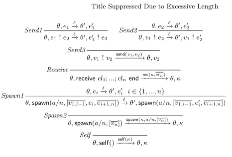
Send1 θ, e1 ` − → θ0 , e01 θ, e1 ! e2 ` − → θ0, e0 1 ! e2 Send2 θ, e2 ` − → θ0 , e02 θ, v1 ! e2 ` − → θ0, v 1 ! e02 Send3 θ, v1! v2 send(v1,v2) −−−−−−−→ θ, v2 Receive θ, receive cl1; ...; clnend rec(κ,cln) −−−−−−→ θ, κ Spawn1 θ, ei ` − → θ0 , e0i i ∈ {1, ..., n}
θ, spawn(a/n, [v1,i−1, ei, ei+1,n]) ` − → θ0, spawn(a/n, [v 1,i−1, e0i, ei+1,n]) Spawn2 θ, spawn(a/n, [vn]) spawn(κ,a/n,[vn]) −−−−−−−−−−−→ θ, κ Self θ, self()−self(κ)−−−→ θ, κ
Fig. 9. Concurrent semantics: evaluation of concurrent expressions.
We use ` to spawn over labels.
We divide the expression rules in two sets, the first one being the set of sequential expressions, depicted in Fig. 8, and the second one being the set of concurrent expressions, depicted in Fig. 9 (by abuse of notation we put self in the second set). As it is in Erlang, we consider that the order of evaluation of the arguments is fixed from left to right.
The sequential expressions define the behavior of some constructs of the language without side-effects, like the case construct, the let binding or the call of a function. Moreover, these rules define the evaluation of an expression inside the data structures of the language (lists and tuples). We label the evaluation of sequential expressions with τ since they can be considered ’silent’ operations and we do not need to distinguish them in the system semantics.
A function in a program can be either defined by the user or built-in. In the former case we exploit rule Apply, where µ maps a function name a/n to its body, in the latter case we apply rule rule Call, where eval evaluates the function.
The only tricky situation in the sequential rules arises in rule Case2, where the auxiliary function match is used. Given an environment θ, a value v, and cln
clauses the function match searches the first clause cli such that v matches pati
and the guard holds.
Now, let us move to the concurrent expressions. Here, we gathered the rules that define the semantics of concurrent operations at the expression level. We can categorize these rules depending on whether we locally know or not to what they reduce. Rules Send1, Send2, Send3 and Spawn1 belong to the first category, indeed we do not need any of the information available at the system level to evaluate them. On the contrary, to evaluate rules Receive, Spawn2 and Self we
Seq θ, e τ −→ θ0, e0 Γ ; hp, θ, e, qi | Π ,→ Γ ; hp, θ0, e0, qi | Π Send θ, e send(p00,v) −−−−−−→ θ0, e0 Γ ; hp, θ, e, qi | Π ,→ Γ ∪ (p00, v); hp, θ0, e0, qi | Π Receiveθ, e rec(κ,cln) −−−−−−→ θ0 , e0 matchrec(θ, cln, q) = (θi, ei, v) Γ ; hp, θ, e, qi | Π ,→ Γ ; hp, θ0θ i, e0{κ 7→ ei}, q\\vi | Π Spawn θ, e spawn(κ,a/n,[vn]) −−−−−−−−−−−→ θ0 , e0 p0 is a fresh pid Γ ; hp, θ, e, qi | Π ,→ Γ ; hp, θ0, e0{κ 7→ p0}, qi | hp0, [ ], id, apply a/n(v
n, [ ]i | Π Self θ, e self(κ) −−−−→ θ0, e0 Γ ; hp, θ, e, qi | Π ,→ Γ ; hp, θ0, e0{κ 7→ p}, qi | Π Sched Γ ∪ {(p, v)}; hp, θ, e, qi | Π ,→ Γ ; hp, θ, e, v : qi | Π
Fig. 10. Standard semantics: system rules.
need information available only at the system level. To tackle the problem, each of these expressions returns a fresh variable κ, which acts like a future, then the system level is in charge of binding κ to its proper value (e.g., the pid of the new process).
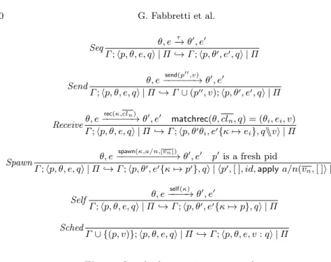
A.2 System level semantics
Fig. 10 depicts the rules of the system semantics, which is defined in terms of the relation ,→. The system semantics defines the behavior of the system, here intended as the global mailbox Γ and the pool of processes Π. Each rule defines how the system can transit from one state to another in a forward manner.
We can see how the system semantics relies on the expression semantics for the evaluation of the concurrent expressions and then how it performs the corresponding action. The corresponding action can be the substitution of κ with its actual value, the application of the appropriate side-effect or both.
Let us consider the case of rule Spawn. In rule Spawn the system level relies on the expression level to evaluate the spawn expression, then it chooses a fresh identifier p as the pid of the new process, replaces κ with p and finally adds to Π the new process.
Now, let us discuss more in detail rule Receive, as it may not be of immediate understanding. The receive construct traverses the queue of messages, from the oldest to the newest, searching for the first message that matches one of the n clauses. If one is found then the receive evaluates to the expression relative to the matching clause, otherwise the process suspends itself. Here, the auxiliary function matchrec, given an environment, a list of clauses, and a queue of
mes-(Seq) θ, e τ −→ θ0, e0 Γ ; hp, h, θ, e, qi | Π * Γ ; hp, τ (θ, e) : h, θ0, e0, qi | Π (Send ) θ, e send(p00,v) −−−−−−→ θ0, e0 λ is a fresh identifier Γ ; hp, h, θ, e, qi | Π * Γ ∪ (p00, {λ, v}); hp, send(θ, e, p00, {λ, v}) : h, θ0, e0, qi | Π (Receive) θ, e rec(κ,cln) −−−−−−→ θ0 , e0 matchrec(θ, cln, q = (θi, ei, {λ, v}) Γ ; hp, h, θ, e, qi | Π * Γ ; hp, rec(θ, e, {λ, v}, q) : h, θ0θ i, e0{κ 7→ ei}, q\\{λ, v}i | Π (Spawn) θ, e spawn(κ,a/n,[vn]) −−−−−−−−−−−→ θ0 , e0 p0 is a fresh identifier Γ ; hp, h, θ, e, qi | Π * Γ ; hp, spawn(θ, e, p0) : h, θ0, e0{κ 7→ p0}, qi | hp0
, [ ], id, apply a/n(vn), [ ]i | Π
(Self ) θ, e self(κ) −−−−→ θ0 , e0 Γ ; hp, h, θ, e, qi | Π * Γ ; hp, self(θ, e) : h, θ0, e0{κ 7→ p}, qi | Π (Sched ) Γ ∪ {(p, {λ, v})}; hp, h, θ, e, qi | Π * Γ ; hp, h, θ, e, {λ, v} : qi | Π
Fig. 11. Forward reversible semantics.
sages, searches for the first message v that matches one of the patterns. When one is found it returns the corresponding environment and expression alongside with the matched message v. Then, the system semantics updates the process’ environment with the new variables introduced by the selected branch, replaces κ with the corresponding expression, and removes v from the process’ queue.
Then, rule Send and rule Sched are the rules that respectively send and schedule a message. More precisely, we apply rule Send every time a process performs a send and, as a side-effect, we update the value of Γ by adding the pair (p00, m), where p00 is the pid of the intended receiver and m is the message. Whereas, by applying rule Sched nondeterministically we remove a message from Γ and we add it to its receiver queue. The fact that rule Sched chooses the pair nondeterministically allows to model every possible interleaving of the messages. Finally, rule Seq denotes a silent operation without side-effects and Self the call of function self by process p.
A.3 A reversible semantics
The forward reversible semantics, depicted in Fig. 11 and defined by the relation *, is the natural extension of the system semantics where each process has been endowed with a history of its previous configurations. More precisely, each time a process performs a forward step, the current configuration and possibly additional pieces of information are saved in the history, then the process transits in a new state.
(Seq) Γ ; hp, τ (θ, e) : h, θ0, e0, qi | Π ) Γ ; hp, h, θ, e, qi | Π
(Send ) Γ ∪ {(p00, {λ, v})}; hp, send(θ, e, p00, {λ, v}) : h, θ0, e0, qi | Π ) Γ ; hp, h, θ, e, qi | Π
(Receive) Γ ; hp, rec(θ, e, {λ, v}, q) : h, θ0, e0, q\\{λ, v}i | Π ) Γ ; hp, h, θ, e, qi | Π
(Spawn) Γ ; hp, spawn(θ, e, p0) : h, θ0, e0, qi | hp0, [ ], id, e00, [ ]i | Π ) Γ ; hp, h, θ, e, qi | Π
(Self ) Γ ; hp, self(θ, e) : h, θ0, e0, qi | Π ) Γ ; hp, h, θ, e, qi | Π
(Sched )
Γ ; hp, h, θ, e, {λ, v} : qi | Π ) Γ ∪ {(p, {λ, v})}; hp, h, θ, e, qi | Π if the topmost rec(...) item in h (if any) has the form rec(θ0, e0, {λ0, v0}, q0
) with q0\\{λ0
, v0} 6= {λ, v} : q Fig. 12. Backward reversible semantics.
The history serves two purposes: it is used to check that all the consequences of the action, if any, have been undone and to travel back in the process’ com-putation.
The only difference, beyond the history, between the forward reversible se-mantics and the system sese-mantics is that in the former each message is uniquely identified by an id, usually denoted by λ or λ0. The need to uniquely identify
each message arise from the necessity to identify a precise point in the past of a process’ computation.
Let us consider the following example to clarify such need.
Example 1. Let us consider three processes p1, p2 and p3; p1 sends a message v
to p2, then p3 sends the same message v to p2. Now, if we desire to undo the
send of message v sent by p1we first need to undo the receive of p2 and to do so
we need to be able to precisely identify the moment in p2’s computation when
it received the message. If the only information available in the process’ history is the content of the message it would be impossible to determine who is the sender of two identical messages.
The problem described in the previous example does not arise if each message is paired with a unique identifier. Indeed, in that case it is sufficient to undo the computation of the receiver up to the receive of the message with the desired identifier. We refer to [18] for a more detailed discussion of the problem.
The uncontrolled backward semantics is depicted in Fig. 12 and defined in terms of the relation ). The backward semantics restores previous states of a process’ computation if all of the consequences of the target action have been undone. In some cases, e.g., rule Seq, since the action does not have conquences we can simply restore the computation without performing any checks. In other cases, e.g., rule Spawn, before undoing a step we need to perform additional checks.
(Seq) θ, e τ −→ θ0, e0 Γ ; hnid, p, h, θ, e, qi | Π; Ω * Γ ; hnid, p, τ (θ, e) : h, θ0, e0, qi | Π; Ω (Send ) θ, e send(p 00,v) −−−−−−→ θ0, e0 λ is a fresh identifier Γ ; hnid, p, h, θ, e, qi | Π; Ω * Γ ∪ {(p00, {λ, v})}; hnid, p, send(θ, e, p00, {λ, v}) : h, θ0, e0, qi | Π; Ω (Receive) θ, e−−−−−−→ θrec(κ,cln) 0 , e0 matchrec(θ, cln, q) = (θi, ei, {λ, v}) Γ ; hnid, p, h, θ, e, qi | Π; Ω
* Γ ; hnid, p, rec(θ, e, {λ, v}, q) : h, θ0θi, e0{κ 7→ ei}, q\\{λ, v}i | Π; Ω
(Self ) θ, e
self(κ)
−−−−→ θ0
, e0
Γ ; hnid, p, h, θ, e, qi | Π; Ω * Γ ; hnid, p, self(θ, e) : h, θ0, e0{κ 7→ p}, qi | Π; Ω
(Sched )
Γ ∪ {(p, {λ, v})}; hnid, p, h, θ, e, qi | Π; Ω * Γ ; hnid, p, h, θ, e, {λ, v} : qi | Π; Ω
Fig. 13. Missing rules of the extended forward reversible semantics
Rules Receive and Sched are the most complicated cases of the semantics, hence let us discuss them in detail. Transitions derived using rules Sched and Receive (applied to the same process) do not commute. In other words, to ensure causal consistency, we must undo them in reverse order of execution. The fact that two applications of rule Sched do not commute is ensured by the fact that we undo a Sched only when the target message is on top of the queue q, hence q is forcing the order. Applications of rule Receive do not commute because we can undo a Receive only when the corresponding item is on the top of the process history. Finally, applications of rules Sched and Receive do not commute thanks to the side condition of rule Sched and since we apply rule Receive only when the queue is the same as when the forward step has been performed.
The other rules are more straightforward. Rule Send can be applied when the message is in Γ because in this case we are sure that each of its consequences has been undone already. Rule Spawn can be applied when the child has an empty history. Finally, rules Seq and Self can always be applied since they never have consequences.
A.4 A distributed reversible semantics
Fig. 13 and Fig. 14 show the missing rules of the semantics depicted in Fig. 3 and Fig. 4. The behavior defined by the rules depicted in the two figures is the same as the one described in Section A.3.
(Seq) Γ ; hnid, p, τ (θ, e) : h, θ0, e0, qi | Π; Ω )p,seq,{s}Γ ; hnid, p, h, θ, e, qi | Π; Ω
(Send ) Γ ∪ {(p
00
, {λ, v})}; hnid, p, send(θ, e, p00, {λ, v}) : h, θ0, e0, qi | Π; Ω )p,send(λ),{s,λ⇑}Γ ; hnid, p, h, θ, e, qi | Π; Ω
(Receive) Γ ; hnid, p, rec(θ, e, {λ, v}, q) : h, θ
0
, e0, q\\{λ, v}i | Π; Ω )p,rec(λ),{s,λ⇓}Γ ; hnid, p, h, θ, e, qi | Π; Ω
(Self ) Γ ; hnid, p, self(θ, e) : h, θ0, e0, qi | Π; Ω )p,self,{s}Γ ; hnid, p, h, θ, e, qi | Π; Ω
(Sched )
Γ ; hnid, p, h, θ, e, {λ, v} : qi | Π; Ω
)p,sched(λ),{λsched}Γ ∪ {(p, {λ, v})}; hnid, p, h, θ, e, qi | Π; Ω
if the topmost rec(...) item in h (if any) has the form rec(θ0, e0, {λ0, v0}, q0
) with q0\\{λ0
, v0} 6= {λ, v} : q Fig. 14. Missing rules of the extended backward reversible semantics